PPT-22 - Climate Science: Roger Pielke Sr.
PPT-22 - Climate Science: Roger Pielke Sr.
PPT-22 - Climate Science: Roger Pielke Sr.

You also want an ePaper? Increase the reach of your titles
YUMPU automatically turns print PDFs into web optimized ePapers that Google loves.
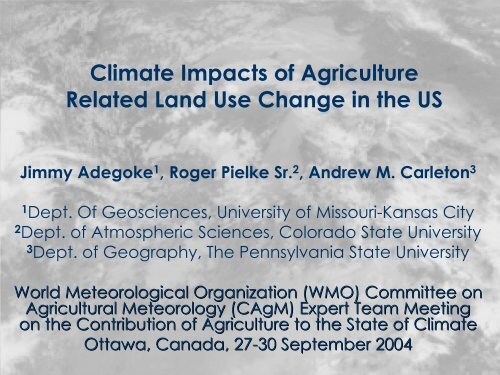
<strong>Climate</strong> Impacts of Agriculture<br />
Related Land Use Change in the US<br />
Jimmy Adegoke 1 , <strong>Roger</strong> <strong>Pielke</strong> <strong>Sr</strong>. 2 , Andrew M. Carleton 3<br />
1 Dept. Of Geosciences, University of Missouri-Kansas City<br />
2 Dept. of Atmospheric <strong>Science</strong>s, Colorado State University<br />
3 Dept. of Geography, The Pennsylvania State University<br />
World Meteorological Organization (WMO) Committee on<br />
Agricultural Meteorology (CAgM ( CAgM) ) Expert Team Meeting<br />
on the Contribution of Agriculture to the State of <strong>Climate</strong><br />
Ottawa, Canada, 27-30 27 30 September 2004
Presentation Outline<br />
Cropland/Forest Impacts on Convective Cloud<br />
Development in the US Midwest : Empirical studies<br />
Agriculture-related land use change impacts on<br />
seasonal climate in the Central US: Modeling studies<br />
Crop-climate modeling Issues, challenges & questions
Current & Potential Natural Vegetation<br />
[Copeland et al., 1996]
Agriculture - Human Imprint on the Land<br />
Surface<br />
Spring Summer
Land Surface-Atmosphere Interactions<br />
Schematic of the differences in surface heat energy budget<br />
and planetary boundary layer over a forest and cropland.
Temp, Water<br />
Trace Gases<br />
Pollutants<br />
Community<br />
Composition &<br />
Structure<br />
Atmosphere<br />
Heat, Moisture<br />
Radiation<br />
Light, Temp<br />
Moisture, Wind<br />
Surface Physiology &<br />
Hydrology<br />
Water & Nutrients<br />
Agriculture<br />
Deforestation, etc.<br />
Biogeochemical<br />
& Hydrological<br />
Cycles<br />
Landscape Modification Anthropogenic Activities<br />
Trace Gases &<br />
Pollutants<br />
Sec - Hours<br />
>1yr - 100yrs<br />
>1000yrs
Focus of Land Surface-<strong>Climate</strong> Work:<br />
Empirical Studies<br />
Impacts of changes in US Midwest land cover<br />
parameters (e.g. land cover, surface roughness,<br />
zones of land cover transitions) on convective<br />
cloudiness (Carleton et al., 2001 GRL Vol. 28, 1679-1684)<br />
Sensitivity of the AVHRR derived Normalized<br />
Difference Vegetation Index (NDVI) and the<br />
Fractional Vegetation Cover (FVC) to growing<br />
season surface moisture conditions (Adegoke and<br />
Carleton, 2002 JHM 4, 24-41).
Wetland<br />
0%<br />
Prairie<br />
2%<br />
Wetland<br />
5%<br />
Prairie<br />
29%<br />
water<br />
3%<br />
Land Use Changes in Illinois<br />
Forest<br />
93%<br />
River<br />
2%<br />
Agriculture<br />
68%<br />
Urban<br />
3%<br />
1820 1980<br />
water<br />
5%<br />
River<br />
0%<br />
Forest<br />
61%<br />
Jackson County<br />
Lake County<br />
Forest<br />
9%<br />
Urban<br />
34%<br />
Prairie<br />
0%<br />
Forest<br />
25%<br />
Wetland<br />
2%<br />
Agriculture<br />
52%<br />
Prairie<br />
0%<br />
Barren<br />
1%<br />
Wetland<br />
2%<br />
Water<br />
1%<br />
Water<br />
2%<br />
Barren<br />
1%<br />
[From Iverson & Risser, 1987]
Land Use/Land Cover Map of The Midwest<br />
Showing Sampling Locations of Convective<br />
Cloud Parameters<br />
…
GOES INFRA RED & VISIBLE IMAGES<br />
11 JUNE 1997 16:00 UTC
Stratification of Case Study Days: June-Aug. 1981-98<br />
Strong Flow / Weak Flow : 500 mb Vector Winds
a) Mean BWF VIS: Crop MI<br />
Albedo<br />
1.00<br />
0.80<br />
0.60<br />
0.40<br />
0.20<br />
0.00<br />
7am<br />
9am<br />
11am<br />
b) Mean BWF VIS: Boundary MI<br />
Albedo<br />
1.00<br />
0.80<br />
0.60<br />
0.40<br />
0.20<br />
0.00<br />
7am<br />
9am<br />
11am<br />
c) Mean BWF VIS: Forest MI<br />
Albedo<br />
1.00<br />
0.80<br />
0.60<br />
0.40<br />
0.20<br />
0.00<br />
7am<br />
9am<br />
11am<br />
1pm<br />
1pm<br />
1pm<br />
3pm<br />
3pm<br />
3pm<br />
5pm<br />
5pm<br />
5pm<br />
295.00<br />
290.00<br />
285.00<br />
280.00<br />
275.00<br />
270.00<br />
265.00<br />
300.00<br />
290.00<br />
280.00<br />
270.00<br />
260.00<br />
250.00<br />
295.00<br />
290.00<br />
285.00<br />
280.00<br />
275.00<br />
270.00<br />
265.00<br />
260.00<br />
Mean BWF IR TEMP: Crop MI<br />
6am<br />
8am<br />
10am<br />
12Noon<br />
2pm<br />
4pm<br />
6pm<br />
Mean BWF IR TEMP: Boundary MI<br />
6am<br />
8am<br />
10am<br />
12Noon<br />
2pm<br />
4pm<br />
6pm<br />
Mean BWF IR TEMP: Forest MI<br />
6am<br />
8am<br />
10am<br />
12Noon<br />
2pm<br />
4pm<br />
6pm<br />
8pm<br />
8pm<br />
8pm
a) Mean BWF VIS: Crop IN<br />
Albedo<br />
1.00<br />
0.80<br />
0.60<br />
0.40<br />
0.20<br />
0.00<br />
7am<br />
9am<br />
11am<br />
b) Mean BWF VIS: Boundary IN<br />
Albedo<br />
1.00<br />
0.80<br />
0.60<br />
0.40<br />
0.20<br />
0.00<br />
7am<br />
9am<br />
11am<br />
c) Mean BWF VIS: Forest IN<br />
Albedo<br />
1.00<br />
0.80<br />
0.60<br />
0.40<br />
0.20<br />
0.00<br />
7am<br />
9am<br />
11am<br />
1pm<br />
1pm<br />
1pm<br />
3pm<br />
3pm<br />
3pm<br />
5pm<br />
5pm<br />
5pm<br />
d) Mean BWF VIS: Crop MO<br />
Albedo<br />
1.00<br />
0.80<br />
0.60<br />
0.40<br />
0.20<br />
0.00<br />
7am<br />
9am<br />
11am<br />
e) Mean BWF VIS: Boundary MO<br />
Albedo<br />
1.00<br />
0.80<br />
0.60<br />
0.40<br />
0.20<br />
0.00<br />
7am<br />
9am<br />
11am<br />
f) Mean BWF VIS: Forest MO<br />
Albedo<br />
1.00<br />
0.80<br />
0.60<br />
0.40<br />
0.20<br />
0.00<br />
7am<br />
9am<br />
11am<br />
1pm<br />
1pm<br />
1pm<br />
3pm<br />
3pm<br />
3pm<br />
5pm<br />
5pm<br />
5pm
a) Mean WF VIS: Crop MI<br />
Albedo<br />
1.00<br />
0.80<br />
0.60<br />
0.40<br />
0.20<br />
0.00<br />
7am<br />
9am<br />
11am<br />
b) Mean WF VIS: Boundary MI<br />
Albedo<br />
1.00<br />
0.80<br />
0.60<br />
0.40<br />
0.20<br />
0.00<br />
7am<br />
9am<br />
11am<br />
c) Mean WF VIS: Forest MI<br />
Albedo<br />
1.00<br />
0.80<br />
0.60<br />
0.40<br />
0.20<br />
0.00<br />
7am<br />
9am<br />
11am<br />
1pm<br />
1pm<br />
1pm<br />
3pm<br />
3pm<br />
3pm<br />
5pm<br />
5pm<br />
5pm<br />
d) Data Range WF VIS: Crop MI<br />
Albedo<br />
1.00<br />
0.80<br />
0.60<br />
0.40<br />
0.20<br />
0.00<br />
7am<br />
9am<br />
11am<br />
e) Data Range WF VIS: Boundary MI<br />
Albedo<br />
f) Data Range WF VIS: Forest MI<br />
Albedo<br />
1.00<br />
0.80<br />
0.60<br />
0.40<br />
0.20<br />
0.00<br />
1.00<br />
0.80<br />
0.60<br />
0.40<br />
0.20<br />
0.00<br />
7am<br />
7am<br />
9am<br />
9am<br />
11am<br />
11am<br />
1pm<br />
1pm<br />
1pm<br />
3pm<br />
3pm<br />
3pm<br />
5pm<br />
5pm<br />
5pm
160<br />
140<br />
120<br />
100<br />
80<br />
60<br />
40<br />
20<br />
0<br />
140<br />
120<br />
100<br />
80<br />
60<br />
40<br />
20<br />
0<br />
140<br />
120<br />
100<br />
80<br />
60<br />
40<br />
20<br />
0<br />
Mean SF VIS Brightness: Crop MI<br />
Mean SF VIS Brightness: Boundary<br />
MI<br />
Mean SF VIS Brightness: Forest MI<br />
120.00<br />
100.00<br />
80.00<br />
60.00<br />
40.00<br />
20.00<br />
0.00<br />
100.00<br />
80.00<br />
60.00<br />
40.00<br />
20.00<br />
0.00<br />
100.00<br />
80.00<br />
60.00<br />
40.00<br />
20.00<br />
0.00<br />
Mean BWF VIS Brightness: Crop MI<br />
6am<br />
6am<br />
8am<br />
10am<br />
12Noon<br />
2pm<br />
4pm<br />
6pm<br />
Mean BWF VIS Brightness:<br />
Boundary MI<br />
8am<br />
10am<br />
12Noon<br />
2pm<br />
4pm<br />
6pm<br />
Mean BWF VIS Brightness: Forest<br />
MI<br />
6am<br />
8am<br />
10am<br />
12Noon<br />
2pm<br />
4pm<br />
6pm<br />
8pm<br />
8pm<br />
8pm
Average Cloud Top Brightness Temperature: MI & MO<br />
102.00<br />
100.00<br />
98.00<br />
96.00<br />
94.00<br />
92.00<br />
90.00<br />
88.00<br />
110.00<br />
108.00<br />
106.00<br />
104.00<br />
102.00<br />
100.00<br />
98.00<br />
BWF Average Maximun Brightness Temp<br />
(MI)<br />
Crop Boundary Forest<br />
BWF Average Maximun Brightness Temp<br />
(MO)<br />
Crop Boundary Forest
Thermodynamic indices for selected “weak flow” days:<br />
12Z Radiosonde Data: MI vs MO<br />
Michigan<br />
Missouri<br />
CCL<br />
(mb)<br />
749<br />
827<br />
CCL-EL<br />
(mb)<br />
480<br />
528<br />
K-Index<br />
(mb)<br />
12<br />
29<br />
Tc ( o C)<br />
32<br />
26.8<br />
Mean<br />
Tv ( o C)<br />
16<br />
20.5<br />
Mean<br />
T-Tv<br />
( o C)<br />
3.7<br />
2.7<br />
RH o / o<br />
68<br />
78<br />
Water<br />
Content<br />
.18<br />
.33
Sensible and Latent Heating of the Atmosphere Required for<br />
Initiation of Convective Clouds vs. Bowen Ratio [Rabin et al., 1990]
Summary of Cloud Research Findings<br />
Analyses of Visible and IR GOES cloud data for<br />
contrasting circulation regimes indicate some<br />
cloud-land cover associations across major<br />
crop-forest boundaries.<br />
Land cover boundary zones are shown to be<br />
favored areas for enhanced cloud development<br />
under moderate mid-tropospheric (< 30 m/s) flow<br />
conditions. The boundary zones tend to behave<br />
like regions of differential vertical circulations (i.e.,<br />
NCMCs)
Focus of Land Surface-<strong>Climate</strong> Work:<br />
Modeling Studies<br />
Improving the representation of land surface<br />
heterogeneity (land cover; soil moisture; soil type) in<br />
the Colorado State University Regional Atmospheric<br />
Modeling System (RAMS)<br />
(Adegoke et al. 2003; Strack et al. 2003; Rozoff et al., 2003)<br />
Developing protocols for a more realistic description<br />
of seasonally and interannually varying vegetation<br />
cover and growth rates in regional climate models<br />
(Adegoke et al. 2004; Eastman et al. 2001; Lixin Lu et al., 2002).
Lessons Learned<br />
Realistic representation of spatial heterogeneity of land<br />
surface parameters improves model simulation of<br />
regional-scale effects of agriculture-related land use<br />
changes on climate and terrestrial biophysical<br />
processes.<br />
Key Parameters:<br />
- Land Cover<br />
- Soil Moisture<br />
-LAI<br />
-Soil Type<br />
- Soil Temperature
Over High Plains, if<br />
model soil moisture is<br />
low<br />
– Forecast CAPE too<br />
low, about half the<br />
observed CAPE<br />
– Forecast of instability<br />
insufficient<br />
Soil Moisture Impacts
Soil Moisture Simulation with Different Soil (a);<br />
Matching Soil (b)<br />
(a)<br />
LDAS Evaluation Team: Alan Robock et al., 2004<br />
(b)
Soil Moisture<br />
LDAS Evaluation Team: Alan Robock et al., 2004
Recent Improvements in RAMS-LEAF2<br />
1. Protocols for ingesting variable soil moisture<br />
2. Incorporation of high-resolution land cover data<br />
(30 m) from the USGS NLCD database<br />
3. Specification of variable soil type from the FAO soil<br />
type database<br />
4. Protocols for ingesting NDVI and derivation of LAI<br />
from NDVI<br />
5. RAMS-Century coupling for explicit modeling of the<br />
seasonal evolution of vegetation in the simulation<br />
of seasonal climate.
Map of U.S. High Plains Aquifer
Acreage of Rain fed & Irrigated Corn Farming in<br />
Nebraska (1950-1988)<br />
Area (ha)<br />
3000000<br />
2500000<br />
2000000<br />
1500000<br />
1000000<br />
500000<br />
0<br />
1950-51<br />
1954-55<br />
1958-59<br />
1962-63<br />
1966-67<br />
1970-71<br />
Rainfed<br />
Irrigated<br />
1974-75<br />
Year<br />
1978-79<br />
1982-83<br />
1986-87<br />
1990-91<br />
1994-95<br />
1998-99
Nebraska Irrigation Modeling Project<br />
Complex changes in the lower atmosphere (PBL)<br />
radiation budget can result from large-scale land use<br />
changes of this magnitude (e.g., vapor flux CAPE)<br />
This study was designed to evaluate the changes in<br />
the summertime surface energy budget & convective<br />
rainfall parameters due to irrigation in Nebraska using<br />
RAMS.
RAMS Modeling Domain<br />
Coarse Grid: 40 km ; Fine Grid:10 km; Domain Height: 20km
a) Kuchler Potential Vegetation b) OGE – Dry Run<br />
c) OGE + Current Irrigation – Control Run<br />
(a)<br />
(b) (c)
Summary of Model Results<br />
Significant inner domain area-averaged difference<br />
between the Control and Dry runs:<br />
- 36% increase in surface latent heat flux<br />
- 15% decrease in surface sensible heat flux<br />
- 28% increase in water vapor flux at 500m<br />
-2.6 o C elevation in dew point temperature<br />
-1.2 o C decrease in near surface temperature<br />
Greater differences observed between the Control<br />
and Natural Vegetation runs e.g.,<br />
- Near ground temperature was 3.3 o C warmer &<br />
surface sensible heat 25% higher in the Natural run.<br />
[Adegoke et al., 2003 Monthly Weather Review 131(3), 556-564.]
ClimRAMS Coupled with CENTURY<br />
(Lu et al., 2001, Journal of <strong>Climate</strong>)<br />
RAMS{temp, swin, prcp, rh, (u,v,w)}<br />
CENTURY{LAI, roots, Zo,<br />
evap, transp, vegfrac, vegalb}
Satellite-derived Leaf Area Index<br />
Derived from AVHRR 10day<br />
composite NDVI<br />
NDVI ⇒ LAI following<br />
Sellers et al. (1996) and<br />
Nemani et al. (1996)<br />
Lu et al., 2001<br />
Derived LAI for Central U.S. in dry (1988),<br />
average(1989), and wet (1993) years.<br />
Average JJA NDVI for Central U.S.
STRONG DIFFERENCES<br />
Magnitude of LAI<br />
Heterogeneity of LAI<br />
SOME DIFFERENCE<br />
Seasonality of LAI<br />
Comparison of LAI Forcing<br />
Lu et al., 2001<br />
Default LAI in Inner (50 km) Grid NDVI-derived LAI in Inner (50 km) Grid
Good Agreement between Model<br />
Predictions & Observations<br />
e.g. Domain-average<br />
maximum and<br />
minimum air<br />
temperature and<br />
precipitation for inner<br />
grid during 1989<br />
(selected as an<br />
“average” year) for<br />
the run with NDVIderived<br />
LAI<br />
Lu et al., 2001
Runs Broadly Agree With Observations<br />
e.g. Distribution of maximum and minimum temperature and<br />
precipitation for inner grid for the run with NDVI-derived LAI<br />
January-March 1989 June-August 1989<br />
Lu et al., 2001
Physical Mechanism for Precipitation Increase<br />
• Lower domainaveraged<br />
LAI allows<br />
more solar radiation<br />
to reach the surface,<br />
increasing CAPE<br />
• Spatial variability in<br />
LAI triggers<br />
mesoscale<br />
circulations.
RAMS-Century Coupling Strategy and Design<br />
• Differences in spatial and<br />
temporal resolutions:<br />
RAMS: 3-D, CENTURY: 1-D<br />
time step: minute vs. day<br />
• Internet Stream Socket<br />
Client/Server mechanism<br />
• Both atmospheric forcings and<br />
biospheric parameters are<br />
prognostic variables<br />
Lu et al., 2001
Coupled Model Captures 2-way Feedbacks<br />
Default<br />
Coupled<br />
LAI response of<br />
CENTURY is different<br />
after harvest when run in<br />
coupled mode. The<br />
coupled model gives a<br />
response in modeled<br />
precipitation.<br />
Lu et al., 2001
Coupled Model Simulated <strong>Climate</strong><br />
Lu et al., 2001
Conclusions From Lu et al. 2001<br />
Both satellite-derived and model-calculated LAI<br />
produce a significant impact on the modeled<br />
seasonal climate<br />
In both cases, the climate is cooler and produces<br />
more precipitation relative to using RAMS default LAI<br />
The effect of heterogeneity in LAI appears to be the<br />
dominant factor in producing these differences<br />
Including realistic description of heterogeneous<br />
vegetation phenology influences the prediction of<br />
seasonal climate.
Looking Ahead<br />
The challenge: Fully coupled crop-climate model<br />
capable of investigating the 2-way interactions of cropclimate<br />
system under a wide range of conditions.<br />
Must include feedbacks of crop growth on surface<br />
climate<br />
Will require much stronger cross-disciplinary<br />
interaction/collaboration between Agricultural and<br />
Atmospheric <strong>Science</strong>s
Discussion Issues/Questions<br />
Crop models tend to operate at the field/plot<br />
spatial scale while climate models typically have<br />
horizontal resolutions of a few km to 100~200 km.<br />
Addressing this spatial scale disparity is not trivial.<br />
Are there additional local terrain and<br />
surface/vegetation characteristics that should be<br />
considered in crop-climate simulations that may<br />
not currently reflected in climate models?<br />
Crop growth parameterization issues: Century vs<br />
CERES-maize model vs General Large Area Model<br />
for annual crops (GLAM)