Efficient post silicon validation via segmentation of the process ...

Efficient post silicon validation via segmentation of the process
variation envelope: Global vs. local variations 1
Abstract—In this paper, we propose an efficient method for incorporating the knowledge of global
(worst case of on-die, across die, across wafers, and across wafer lots) and local (worst case on-die) process
variations into a systematic framework for identifying delay marginalities in a design during first-silicon
validation. With the goal of significantly reducing the number of vectors required for validation, we
propose an approach for segmenting the normal process variation envelope into sub-envelopes, where each
sub-envelope is guaranteed to capture worst-case local variations, and where all sub-envelopes collectively
capture the worst-case global variations. We then use our recent approach for generating multiple vectors
(vector-spaces) [15] in a segment-by-segment manner to guarantee the invocation of the worst-case delay
of the chips in the first-silicon batch. We present extensive experimental results to demonstrate the
effectiveness of our approach, especially in the context of increasing process variations.
Keywords: delay marginalities, first silicon validation, local and global process variations, and
segmentation of process variation envelope.
1 This research was supported by Intel Corporation.
Prasanjeet Das and Sandeep K. Gupta
Department of Electrical Engineering – Systems
University of Southern California
Los Angeles CA 90089
prasanjd@usc.edu, sandeep@poisson.usc.edu
1

I. INTRODUCTION
The development of a new digital chip starts with its specifications, which describe the desired
functionality and key parameters, such as performance and power (see Figure 1). A multi-step design
process produces a detailed design in the form of a gate/transistor-level netlist and a layout. In most existing
flows for custom or semi-custom design, the quality of chips shipped to customers is ensured via a sequence
of three processes, namely pre-silicon verification of a chip‘s design, post-silicon validation of the
first-silicon for the design and testing of each fabricated copy when the design is fabricated in high
volume[1]. Any misbehavior identified during validation that is deemed likely to cause a significant
fraction of fabricated chips to fail (and hence threaten the chip‘s economic viability) is addressed via
redesign. Each such redesign is commonly referred to as a new silicon spin. Such redesign is expensive and
time-consuming, since it requires diagnosis to identify the root cause, redesign, creation of a new set of
masks, and re-fabrication. When validation is eventually successful, the corresponding set of masks is used
to manufacture chips in high volume.
Specifications
Design
Detailed design:
Netlist and layout
Verification
Initial
fabrication
First-silicon
Figure 1: A typical design flow. (Solid arrows show flow of design information, while dashed arrows indicated
re-design/go-ahead signals.)
2
Validation
High volume
fabrication
Chips
Testing

Despite advances in design and verification, it is becoming increasingly common for many chip designs
to undergo multiple silicon spins. This is the case not only for high-performance custom and semi-custom
chips but also for application-specific integrated circuits (ASICs), which are typically much less complex
and much less aggressive in terms of area efficiency and performance. For example, as reported in[2][3],
Collett International Research reports that 37% of ASICs require a second spin while 24% of ASICs require
more than two spins (see Figure 2). Similar data from Numetrics Management Systems, Inc. has been
presented in [4]. The fact that multiple silicon spins are required [4] implies that it is becoming increasingly
common for many causes of serious circuit misbehavior that can cause significant reduction in yield to be
first discovered during validation, in particular marginalities, are gaining importance. As the fabrication
process pushed to its limits, marginalities (defined in Section II) will continue to grow in importance for the
foreseeable future, rendering existing validation approaches inadequate. Hence the primary emphasis of our
systematic framework is on the development of a high quality validation methodology that is guaranteed to
detect all possible serious causes of circuit misbehavior (delay marginality being the one addressed here)
which threaten a chip‘s economic viability.
Figure 2: Most ASICs require multiple silicon spins. (Source: Collett International Research cited in [2][3]).
For historical reasons, existing validation approaches largely target design errors missed by verification.
In particular, existing validation approaches use functional, pseudo-random, and biased random vectors as
well as verification test-benches [5][6]. Most approaches do not quantify the quality of vectors. Few
3

approaches that do quantify do not consider marginalities but use logic- and higher-level metrics adopted
from software testing [7] and high-level verification [6], such as HDL statement/block coverage.
Furthermore, none of the existing approaches generate vectors with the objective of invoking worst-case
severities for low-level effects that are behind marginalities.
Delay marginality is one such effect which eventually leads to slow ICs. Path delay test (PDT) has
traditionally been believed to be superior in finding slow paths and considered to be more useful for speed
binning and performance characterization. However, recent silicon studies reported by nVidia [8],
Freescale [9] and Sun [10] have shown that existing path delay testing approaches generate vectors that fail
to invoke the worst-case delays in first-silicon. Existing approaches for generating vectors for testing for
other low-level effects, such as capacitive crosstalk and ground bounce [11][12], use nominal values for
parameters and parasitics. This makes the generated vectors non-resilient, i.e., unreliable for any fabricated
copy of the chip, and hence unsuitable for validation.
Because of increased complexity of semiconductor manufacturing process and the atomic scale control
required to fabricate modern transistors and interconnects, it is becoming increasingly difficult to control
values of parameters [20]. Hence process variations are becoming an increasing concern for both analog
and digital designers [13] (Figure 3 shows the delay variability on various implementations of 16 bit adders
on 90 nm technology node from [24]).
ITRS [14] shows and predicts that the amount of variations in key parameters increases as the minimum
dimensions shrink, making it imperative to develop a validation approach that is resilient, i.e., one that will
not be invalidated by increasing process variations. The fact that the increase in importance of marginalities
– aggravated by process variations, will continue unabated for the last years of CMOS scaling is also clearly
evident from the amount of research effort devoted to related concerns (e.g., see the Proceedings of IEDM
for any recent year). The importance of our approach will increase even more dramatically when new
technologies start replacing or supplementing CMOS. While the technologies that might eventually replace
or supplement CMOS are still in their infancy, it is already clear that each will be plagued by
corresponding low-level effects and process variations to an even greater extent. For example, in some
4

technologies, reliable circuit operation can be obtained only when the functional circuit is supplemented by
redundant circuitry whose total size is many times the size of the functional circuit (e.g., see [21]).
Figure 3: Normalized delay variability for 16-bit adders [24]
In [15] we presented a systematic approach to generate a set of multiple vectors, called test
vector-spaces, for high quality post silicon delay marginality validation of high performance designs. In
particular, our approach guarantees invocation of the worst-case delay of the chips in first silicon batch.
However, we show (in Section IV) that the number of vectors generated by this approach increases
dramatically with increase in process variations. In this paper we develop a new approach to incorporate the
knowledge of global and local variations into this methodology with the goal of significantly reducing the
5

cost of first-silicon validation. While we focus on validation for delay marginalities in this paper, the
proposed approach is useful for resilient validation of any other type of marginality.
This paper is organized as follows. In Sections II and III we present the necessary background and the
previous works respectively. In Section IV, the motivation and importance of our new approach is
presented. In Section V, our overall approach for segmentation of process variation envelope is presented.
The experimental setup and results are described in Section VI. Finally, conclusions are presented in
Section VII.
II. BACKGROUND
A. Factors affecting chip behavior
A chip may have erroneous behavior due to (i) design errors, (ii) marginalities, and (iii) defects. A design
error is a logic error or a gross delay problem in a design that causes an unacceptable deviation from desired
functionality or a catastrophic reduction in yield. A marginality is any aspect of a design that makes it
probable that a significant fraction of fabricated chips will have erroneous behavior, even in the absence of
defects and even when the variations in the fabrication process (process variations) are within the
normally expected levels, i.e., even when there is no abnormal process drift. Low-level effects, such as,
delay variations, inadequate noise margins, excessive leakage currents, charge sharing, ground bounce,
crosstalk, and inherently stochastic behavior, are root causes of marginalities. The severity of each such
effect depends on the values of circuit parameters and parasitics and may be aggravated by process
variations. Finally, fabrication defects, including abnormally high process variations, may cause some
chips to have erroneous behavior.
B. Timing uncertainty and delay variations
The uncertainty of timing estimate of a design can be classified into three catagories [23] (see Figure 4):
1. Modeling and analysis errors – inaccuracy of device models, in extraction and reduction of
interconnect parasitics, and in timing analysis algorithms.
6

2. Manufacturing variations–uncertainty in parameters of fabricated devices and interconnects
from die to die and within a particular die.
3. Operating context variations–uncertainty in the operating environment of a particular device
during its lifetime, such as temperature, operating voltage, mode of operation and life-time
wearout.
Figure 4: Steps in design process and their effect on timing uncertainties [23]
In this paper we focus primarily on the timing uncertainty due to process variations, specifically delay
marginality which is an important variation induced timing bug that contributes to a significant fraction of
circuit bugs detected by validation. As shown in Figure 5, parameter variations lead to electrical variations
which in turn lead to delay variations (delay marginality).
C. The taxonomy of process variations
Figure 5: Parameter variations causing delay variations [23]
The main sources of process variations (variability) in current general-purpose CMOS processes are [16]:
1. Random dopant fluctuation (RDF) – The fluctuation of the number of dopant atoms leads to
variation of observed threshold voltage Vth for the transistor. RDF is regarded as the major source
of device variation in DSM technology node.
7

2. Line edge roughness (LER) – It is the local variation of the edge of polysilicon gate along its
width. The causes of increased LER include the incoming photon count variation during
exposure and the contrast of arial image, as well as the absorption rate, chemical reactivity, and
the molecular composition or resist.
3. Oxide thickness variation (OTV) – In DSM technology node, the thickness of oxide layer is
countable number of atomic-level roughness of oxide-silicon interface layer which is becoming
increasingly difficult to control. This leads to increasing variation in device parameters like
mobility and threshold voltage.
Figure 6: General taxonomy of variation
Process variations is also referred to as variability.The variability can be mainly categorized as per the
terminology used in [16] as follows (see Figure 6).
Systematic process variation – the behaviour of these physical parameter variations have been
well-understood and can be predicted apriori, by analyzing the layout of the design. The
examples are variations due to optical proximity, CMP and metal fill etc.
Non systematic process variation – these have uncertain or random behaviour and arise from
processes that are orthogonal to design implementation. The examples are the primary
contributor to process variations RDF, LER, OTV.
8

Environmental variation – includes power supply voltage and temperature variations.
It is common practice in design flow to model systematic variations deterministically (in the advanced
state of design after gaining more information) and to model the non-systematic variations statistically.
Depending on the spatial scale of variations, process variations can be further classified.
1. Global variation (on-die as well as inter-die, inlcuding die from different wafers and different
wafer lots)–The die-to-die variations result in shift in the process from reticle to reticle, wafer to
wafer, and lot to lot. For example, gate length variation of all the devices on the same chip being
larger or smaller than the nominal value.
2. Local variation (within-die or intra-die) – Variations affect each device within a die differently.
For example, some devices on a die have smaller gate lengths whereas other devices on the same
die have a larger gate lengths. Clearly local variations are lower than global variations, since the
former is subsumed by the latter.
The within-die variations can be further classified as:
1. Spatially correlated variations–The kind of within-die variations which exhibit similar
characteristic for devices in small neighborhood in the die than those are placed far apart.
2. Random or independent variation – The kid of within-die variations which is statistically
independent from other device variations. Examples are RDF and LER.
Figure 7: Categorization of device variation [24]
9

The table in Figure 7 [24] shows the industry specific categorization of device variability for 65nm. Here,
variations are separated into rows according to spatial domain: those that involve chip mean (global), those
that vary within the chip (local) but have local or chip-to-chip correlation, and those that vary randomly
from device to device (local). The columns identify variations arising from the process used to make the
device, or originating from device behavior changes over time. Such a categorization of variability is useful
as it separates issues requiring different statistical treatments in anticipating their circuit impacts.
D. Terminology and definitions
In this paper, combinational circuits comprised of primitive gates are considered. We start by presenting
the basic terminology and definitions [17].
Logic value system: Throughout this paper we deal with sequences of two vectors, even though for
simplicity we often refer to them as vectors.
Hence we denote logic values at a line by using a subset of {CF, CR, S0, S1, TF, TR, H0, H1}, where CF
stands for clean falling (no hazard), S0 stands for static 0 (no hazard), TF stands for transition to value 0
(dynamic hazards possible), and H0 stands for hazardous 0 (static hazards possible). CR, S1, TR, and H1
are similar.
Controlling value (CV): The controlling value of a multi–input gate is the logic value which when
applied to any one of the gate‘s inputs, uniquely determines its output value. NCV represents the gate‘s non
controlling value.
The to-controlling transition at an input of a multi-input gate is a transition from logic value NCV to CV.
To-non controlling transition is similarly defined.
Logical path (P): A logical path (P) is a sequence of lines along a circuit path L1 (a primary input), L2, …,
and Ln (a primary output) and a set of signal transitions Tr1, Tr2, …, and Trn, where Tr {R, F}, such that Tri
represents the signal transition at Li.
10

III. PREVIOUS WORK
A. Work on variability
Increasing importance of variability on delay and power consumption in CMOS circuits is addressed
comprehensively in [24]. Statistical approaches [25] have evolved over time to effectively analyze
variability and associated effects. Considerable amount of existing and ongoing research addresses design
specific traits such as variability aware design [26], statistical timing analysis [23], statistical cell
characterization [27], statistical leakage prediction [28], statistical path selection [29] and even variability
aware subthreshold/near-threshold design [30]. Recently, researchers such as [31][32][15] have started
addressing test specific traits such as variability-aware fault modeling, delay testing and delay validation
respectively. Works such as [33][34] present pre-silicon variation models where the spatially correlated
component of within-die variations are addressed using grid-based models. [35] Presents an active learning
framework for post-silicon variation modeling and [36] shows how PDF (Probability Distribution
Function) for total variation can be arrived at by using weighted sum of local variation PDFs at discrete
points on global variation PDF. Hence considerable amount of work has been done on design domain
[36][37][23], to incorporate knowledge of global and local process variations but similar efforts on the
testing domain haven‘t been made till now. To the best of our knowledge, ours is the first approach that
evaluates the effectiveness of incorporating global and local variation specific information in a delay testing
and validation framework.
B. Recent silicon studies
We have already reviewed shortcomings of the existing approaches in Section I and since we were
primarily interested in the validation of high performance circuits, in [15] we summarize several silicon
experiments from industry [8][9][10] to understand the limitations of the path delay testing when used to
characterize the timing behavior of logic circuits. One common observation from the results of [8][9][10] is
that, contrary to widespread expectations, the PDTs invoke lesser delay than functional tests, since the
actual critical paths in silicon are different from the paths identified by STA.
11

The following four reasons are evident from [8][9][10] for this anomaly viz-a-viz expectations:
Inaccurate and non resilient delay models.
Incorrect path selection approaches
Wrong path sensitization conditions
Use of statically sensitized robust PDTs that do not guarantee invocation of the worst-case delay
for a target path.
Besides these, other reasons such as test application differences, pre silicon – post silicon netlist
mismatches and many more also contribute to the observed anomaly.
Though our work primarily deals with marginalities (aggravated by process variations) and not faults, a
systematic and deterministic PDT approach, where the shortcomings of the general approach are removed
will be a suitable candidate for our framework.
C. Our recent framework for detecting delay marginalities
Phase 0: Path selection
Given a value of TTout (= TC – (Δ ± ρ)), identify timing sensitive (target) paths (TPs).
Phase 1: Cone exhaustive
For each TP identified in phase 0, mark the fan in cone.
Phase 2: EFS
Apply enhanced functional sensitization conditions to the TP and eliminate the TP if the
conditions cannot be satisfied after implications
Phase 3: MDS
Apply maximum delay sensitization conditions to the TP and eliminate the TP if the
conditions cannot be satisfied after implications; otherwise, arrive at the ―mother‖ test
vector-space for the TP.
Phase 4: SIR
Refine each side input based on the partial ordered graphs and arrive at a set of non
inferior vector sub-space for the TP.
Phase 5: TBP
Perform timing based pruning to identify primary inputs where values to be enumerated
to arrive at the number of fully specified patterns.
Figure 8: An overview of our 6-phase approach
12

In [15] we presented a new six phase systematic approach (Figure8) for identifying a set of multiple
vectors (MV) known as a test vector-space guaranteed to resiliently detect the target path with no
pessimism, even if loose bounding approximation models are used to derive or analyze vectors.
The overall approach has four main components:
1. Resilient delay model
Our approach uses a resilient delay model, i.e., a delay model that will not be invalidated by
inaccuracies and variations as it captures the inaccuracies and variations in delay parameters using
bounding approximations. The delay model proposed in [17] only uses qualitative information such as the
causality property along with provable properties of underlying physics, such as the effects of
near-simultaneous transitions at multiple inputs of a gate, and hence is a suitable candidate for our
framework. But a single curve as proposed in [17] cannot capture all inaccuracies and variations, we need
an envelope comprising of two curves – one upper bound and one lower bound – to bound all inaccuracies
and effects of process variations [18].The inaccuracies and variations in these delay parameters can be
captured using bounding approximations where the inaccuracies at each circuit line are bounded by ±ρ%,
where ρ captures inaccuracies in circuit parameters [19] such as Vth, Leff, tox, and so on. Our approach
expresses variability in terms of the parameters of the devices in the gates. Using the value of device
variability from the given industry standard 65nm library, we perform Monte Carlo simulations to obtain
the two envelopes to bound the gate delay as illustrated in delay curves of Figure10(a), Figure10(b) (details
can be found in [18]).
2. Path selection
We use a path selection approach that uses our resilient delay model to identify a set of paths that is
guaranteed to include all paths that may potentially cause a timing error if the accumulated values of
additional delays along circuit paths is upper bounded by a desired limit [22].
3. Timing and logic conditions for guaranteed invocation of worst-case delay of a target path
In [15] we arrived at the necessary timing and logic conditions (MDS conditions – see Table 1) that will
guarantee invocation of worst case delay at each gate along a target path. In contrast to robust conditions
13

[8], our approach starts with the set of all possible values and eliminates only those cases that can be proven
as being unable to invoke the worst-case delay under any circumstance.
Table 1: MDS conditions for a to-non-controlling transition at on path input of a 2-input NAND gate
4. Selective enumeration
Timing Case Logic Conditions
1. Y before X and not near simultaneous {CR, TR, S1, H1}
2. Y before X and near simultaneous but no overlap {CR, TR, S1, H1}
3. Y overlaps X {CR, TR, S1, H1}
4. Y after X and near simultaneous but no overlap {CR, TR, S1, H1}
5. Y after and not near simultaneous { S1, H1}
Using partial ordering (based on the worst case delay invoked) [15] among the logic conditions for
sensitization, we develop an innovative search algorithm to arrive at a set of multiple vectors that will
resiliently invoke maximum delay of the target path.Figure9shows the partial ordered graphs for timing
case 1 and 2 shown in Table 1.
1
{S1, CR, H1, TR}
Figure 9: Partial ordered graph for all side input values for timing case 1 and timing case 4
Using the partial ordered graphs we refine the logic values at side inputs to arrive at a set of multiple
vectors, termed as a test vector-space, guaranteed to resiliently detect the target path. A test vector-space is
a partially-specified vector where designated partially-specified values are expanded into all possible
combinations and every one of them will be applied during validation. For example, if the first two
partially-specified values in xxd10 are designated as ‗x‘ for expansion while the third is designated as ‗d‘
for don‘t care, then our validation vector set comprises of the following four partially-specified vectors:
00d10, 01d10, 10d10, and 11d10, where d is don‘t care and can be replaced by either 0 or 1.
We eliminate only provably inferior (low delay invoking) vectors in our approach and hence our test
vector-spaces comprise of sets of non inferior vectors that are collectively guaranteed to resiliently detect a
target. Our all inclusive approach selects all non inferior vector sub-spaces as suitable candidate for
14
{CR}
2
{H1}
{S1}
{TR}

validation. The search starts by enumerating the values at each side input and reducing them to either a
single value or a single equivalent set. At the leaf node of our search tree, it deals with the elimination of
inferior vector sub-spaces and storage of non inferior vector-spaces.
IV. PREVIOUS WORK
A. Work on variability
Increasing importance of variability on delay and power consumption in CMOS circuits is addressed
comprehensively in [24]. Statistical approaches [25] have evolved over time to effectively analyze
variability and associated effects. Considerable amount of existing and ongoing research addresses design
specific traits such as variability aware design [26], statistical timing analysis [23], statistical cell
characterization [27], statistical leakage prediction [28], statistical path selection [29] and even variability
aware sub-threshold/near-threshold design [30]. Recently, researchers such as [31][32][15] have started
addressing test specific traits such as variability-aware fault modeling, delay testing and delay validation
respectively. Works such as [33][34] present pre-silicon variation models where the spatially correlated
component of within-die variations are addressed using grid-based models. [35] Presents an active learning
framework for post-silicon variation modeling and [36] shows how PDF (Probability Distribution
Function) for total variation can be arrived at by using weighted sum of local variation PDFs at discrete
points on global variation PDF. Hence considerable amount of work has been done on design domain
[36][37][23], to incorporate knowledge of global and local process variations but similar efforts on the
testing domain haven‘t been made till now. To the best of our knowledge, ours is the first approach that
evaluates the effectiveness of incorporating global and local variation specific information in a delay testing
and validation framework.
V. MOTIVATION
This paper is motivated by the clear trend that, marginalities constitute an increasing proportion of
misbehavior first discovered during validation. This increase in importance of marginalities is caused by
low-level effects and is aggravated by process variations. Going along these lines we decided to
15

incorporate the effect of process variations on our validation approach [15] for 65nm technology node. In
our experiments on the ISCAS89 benchmark c17 (17 lines and five primary inputs) we consider local
variability as well as full global variability. For each level of variations, we select the top 10% delay paths
(∆ = 0.1) to generate the validation vector-space using our recent approach [15] outlined above.
Figure 10(a): Validation vector generation for c17 for local variability
Figure 10(a) shows the value at each circuit line at the end of our approach for generating test vector
spaces for validation [15] for the logical path {R3, R7, F9, F10, R12, R13, F16} as well as the resilient delay
model curves for local variability. The number of vectors generated is 1*1*1*1 = 1. Figure 10(b) shows the
same information for the same path for the case for full global variability. In this case, the number of vectors
increases to 2*2*1*2 = 8. While the increase in number of vectors for a path is small (from 1to 6) for a small
circuit like c17, we also explored the effect of increasing levels of variations for slightly larger circuits (the
increase in number of vectors required for a single top critical path in ISCAS89 benchmark s1196 is
reported as 3,478).
Figure 10(b): Validation vector generation for c17 for full global variability
16

Table 2 shows the effect of variations on paths selected and vectors generated for several of medium sized
ISCAS89 benchmarks (∆ = 0.1). It should be noted that the results in Table 2 corresponds to the number of
paths selected and the number of vectors generated after we have finished justification procedure [15]
where certain paths are aborted because of the provided backtrack limit.
Table 2: Effect of variations on paths selected and the number of validation vectors
Paths selected Vectors generated
Nominal
Local
variations
Full global
variations
Nominal
Local
variations
Full global
variations
s298 9 13 20 9 22 154
s444 1 7 22 1 7 22
s713 7 17 38 1 162 3,422
s953 3 12 47 6.5 x 10 4 1.43 x 10 5 1.73 x 10 7
s1196 12 26 52 44 1,622 16,542
It is evident from Table 2 that as the levels of variations increase from local variations to global variations,
the number of paths that must be targeted as well as the number of vectors generated for validation of each
target path increase dramatically. This empirical observation prompted us to identify key properties
pertaining to the effects of increasing levels of variations on various steps of our approach for generating
validation vectors. Since our approach uses a resilient delay model [18] whose envelopes encapsulate all the
points of variability on the basic delay model proposed in [17], we identified its following key properties:
As variations increase (super-set), the envelopes expand and subsume all the points in the
envelopes for lower levels (sub-set) of variations. Thus the envelopes of full global variability
subsumes the envelopes of local variability.
With increase in variations (super-set), the timing ranges (calculated by our ETA [22]) at each
circuit line are a super-set of those for lower levels of variations (sub-set).
As the threshold (Δ) increases, the number of paths identified as targets for validation increases.
With increase in variations, the number of paths in the target set that are functionally sensitizable
(FS) and maximum delay sensitized (MDS) increases.
With the increase in variations, the size of the mother vector-space [15] (obtained after MDS, but
before SIR) either expands or remains constant.
17

With the increase in variations, the test vector-spaces expand and hence so do the total number of
vectors needed for validation of the complete circuit. In particular, with higher variations, our
timing conditions call for more side input refinement. Subsequent implications call for enumeration
at additional circuit lines, compared to lower variations. The search space for the non-inferior test
vector-spaces expands as the set of logic conditions provide more values to be enumerated.
As evident from Table 2 and the properties identified above, as the variation grows, the number of
testable paths identified grows and so does the number of vectors in the validation vector-space for each
testable path. Hence, it is imperative to develop an approach to reduce the number of vectors required for
validation of marginalities, without compromising its resilience.
VI. PROPOSED APPROACH
A. Global vs. local variations
As mentioned earlier, global variations equally affect parameters of all devices on a particular chip. On
the other hand, local variations affect differently the parameters of each individual device on a chip. Further
local systematic variations affect devices differently depending on whether these devices are placed near or
far away from each other [38]. In [39][40] it is shown that the size of biggest combinational logic block in
industry standard 65nm technology is within the area of 100μm x 100μm (considered to be dominated by
the local nearby component of local variations). Thus for our proposed approach (focusing only on the
combinational part of logic blocks) we assume local variations to be comprised of local nearby variations
only. In the rest of the paper global variations will be referred to as global variability and local variations
will be referred to as local variability.
From the previous section it is evident that as the variability increase from local to global, the number of
vectors in the validation test set increases. So we propose an approach to segment and quantize the global
variability envelope, based on the information regarding local variability. Our approach is based on the
assumption that ring-oscillator based test structures or process monitors such as [41][42] to estimate the
global process shift on delay values are generally present on most of the fabricated chips.
18

B. Segmentation of the variations envelope – The divide and conquer approach.
Full global variability comprises of two components namely global variability only and local variability
only as shown in the left hand side of Figure 11 (Here we assume that all components of variability can be
approximated as normal distribution for reasons explained later ).
Figure 11: Uniform segmentation of full global variability envelope (single parameter).
We propose to arrive at the full global variability using a segmented approach where the global
variability only component (μG, σG) is segmented into many segmented envelopes and the full global
variability (μL, σL) can be arrived at by weighted/non-weighted sum of contributions from the segmented
envelopes (similar to the concept of weighted sum at discrete points in [36]).
Based on the sizes of individual segments, the segmented approach can be classified as:
Uniform segmentation – segmented sections are of uniform width - kσ (e.g., Figure 11 shows
uniform segmentation with three segments of width 2 sigma (σ) each.
Non-uniform segmentation – segmented sections are of varying widths – k1σ, k2σ, … (e.g.,
Figure 12 shows uniform segmentation with four segments, where the central segment is of
width σ, and the segments at the extremes are of width 2.5σ each. We propose to segment at
higher granularity at center as the concentration of chips will be much more near the center than
at the extremes.
19

Note that the weighting is done as per the area under the curve (probability of occurrence of the nominal
operating point of the fabricated chip within the segmentized interval).
Figure 12: Non-uniform segmentation of full global variability envelope (single parameter).
As mentioned earlier, our approach expresses variability in terms of the parameters of the devices in the
gates. Transistor threshold voltage (Vth) is the most dominant contributor to device variability for the
transistors used in today‘s CMOS gates [19][24] and can be considered as a basis for segmentation. From
Section IV, it is evident that as the global variations increase, the number of vectors in the validation test set
increases. So we propose an approach to segment and quantize the full global variation envelope, based on
the information regarding local variations. A uniform three-way and non-uniform three-way segmentation
can be performed on the single device parameter Vth as shown in Figure 11 and Figure 12 respectively.
Later we will show the benefits of segmentation on ISCAS benchmarks which is evident from the fact that
even for a small benchmark such as c17, the one parameter (Vth) three-way segmentation based adaptive (to
be explained next) approach can reduce the validation vector set by as much as 5X (15 to 3).
20

Figure 13: Uniform segmentation of full global variability envelope (two parameters – V th and L eff).
Ideally, all possible sub-envelopes within global variability envelope must be considered. But, since there
are an infinite number of such sub-envelopes, we need to simplify test development (smaller path- and
vector-sets for validation) by quantizing the nominal operating points for which we consider a
sub-envelope. We consider the nominal operating points to be at the extremities of each sub-envelope.
Hence for the case in Figure 11, the nominal operating points will be shifted corresponding to global
variability component at -3σ, -σ, +σ and +3σ.
Based on the number of parameters considered during segmentation, the segmented approach can be
classified as:
One parameter segmentation ( segment along Vth)
Two parameter segmentation ( segment along Vth as well as Leff)
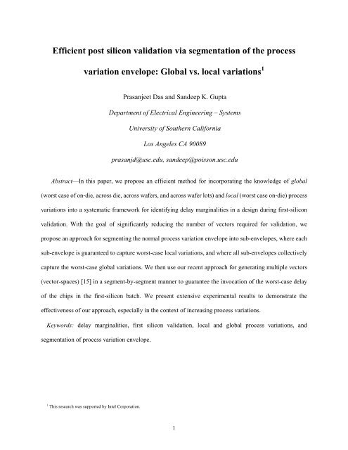
Figure 13 shows the 3 way (uniform) segmentation for the two dominant delay variability parameters –
Vth (horizontal) and Leff (vertical). Note that the two probability distribution functions (green) in Figure 13
are corresponding to Vth and Leff; respectively, and the horizontal and vertical axes of the square represent
the spread of full global variability for Vth and Leff; respectively. Consider the full global variability
envelope (left) of {(-3σ, +3σ) for Vth and (-3σ, +3σ) for Leff} being represented as a set of 36 small
rectangles, namely, 1A to 6F in Figure 13.A set of 4 small rectangles, e.g., 3C to 4D in Figure 13 (right)
21

epresent a global variability sub-envelope of size 2σ*2σ{(-σ, +σ) for Vth and (-σ, +σ) for Leff}. Note that
3-way segmentation in two parameters will correspond to 3*3 = 9 sub-envelopes (from 1A-2B to 5E-6F),
similarly for n parameters there will be 3 n sub-envelopes covering the n-dimensional full global variability
surface.
Figure 14: Non-uniform segmentation of full global variability envelope (two parameters – V th and L eff).
Figure 14 shows the 3 way (non-uniform) segmentation for the two parameters – Vth (horizontal) and Leff
(vertical). We have 9 sub-envelopes of varying sizes (four of size 6.25σ 2 , four of size 1.25σ 2 , and one of size
σ 2 as shown in Figure 14) for such cases.
Figure15: Illustration of sub-envelopes of different sizes (single parameter uniform segmentation)
Also based on the number of segments generated, the uniform segmented approach can be classified as
22

either 3-way segmentation or 6-way segmentation (Figure 15). Similar classification for non-uniform
segmentation is shown in Figure 16.
Each of the 9 squares (1A-2B to 5E-6F) in Figure 16 (a) represent a variability sub-envelope of size
2σ*2σ {for example sub-envelope 3C-4D corresponds to (-σ, +σ) for Vth and (-σ, +σ) for Leff} for 3-way
segmentation whereas each of the 36 squares (1A-1A to 6F-6F) in Figure 16(b) represents a sub-envelope
of size σ*σ {for example sub-envelope 4D-4D corresponds to (0, +σ) for Vth and (0, +σ) for Leff} for 6-way
segmentation .
Figure16: Illustration of sub-envelopes of different sizes (two parameters– uniform segmentation)
Figure 17 shows non-uniform segmentation on one parameter at higher granularities,where the whole
global variability envelope is divided into 6 sub-envelopes. Along the same lines 6-way non-uniform
segmentation with two parameters will lead to 36 sub-envelopes of varying sizes.
Figure17: Illustration of sub-envelopes of different sizes (single parameter non-uniform segmentation)
23

Segmentation can be done at more granular level but this will increase the complexity of all the parts of
our framework from preprocessing step of characterization of resilient delay model to the final step of
generating vectors. Also, with the increase in number of variability parameters considered the complexity
exponentially grows. Later in the section of Experimental results we will show that segmentation at this
granularity gives us about 10X reduction in validation vector volume without any explosive increase in
complexity of our framework.
C. Segmentation of the variations envelope – usage of sub-envelopes during characterization, path
selection, timing analysis and vector generation
Figure 18: Uniform segmentation of full global variability envelope including full local variability
(two parameters – V th and L eff).
The full global variability envelope shown in Figure 13 and Figure 14 is incomplete; it shows only how
the global variability envelope is segmented. The actual full global variability envelope will be arrived at by
superimposing the full local variability envelope at the quantized points (which are the extremities of the
segmented global variability envelope) corresponding to each sub-envelope. Such an arrangement for
3-way segmentation (uniform) corresponding to Figure 13 is shown in Figure 18. The complete full global
variability envelope is given by the large rectangle on the left side; the nine sub-envelopes are given by the
24

overlapping rectangles shown on the right side of Figure 18. Note that the extended rectangle represents the
effect of local variability on top of global variability.
D. Segmentation of the variations envelope – usage of sub-envelopes during validation
The variations in each parameter are typically modeled by a distribution. Normal distribution is often
assumed, since it is often a fairly good approximation of the empirical reality and simplifies analytical
derivations. In such cases, the numerical value of global variations in a parameter, may correspond to some
multiple of its standard deviation, typically, 3σ or higher. In such a scenario, we have the following
important observations.
1. The full global variability envelope does not denote the entirety of all possible variations. For
example, if we assume that the numerical values for each parameter in the example in Figure 18
correspond to the 3-times the standard deviation for the respective parameter, and then the full
global variability envelope in Figure 18 represents 99.4% of all possible chips fabricated using that
process.
2. Each sub-envelope in Figure18 denotes die with different nominal values of its parameters as well
as the worst-case local variability. The size of sub-envelope must be greater than or equal to the
worst-case local variations so as to ensure resilience of the vector-spaces generated. We adhere to
this rule as for each segmented envelope we consider the full local variability possible for that case
and only divide the global variability envelope (Figure 18).
3. Each sub-envelope, such as those shown in Figure 13 (Figure 18), represents sets of die that may be
fabricated with different probabilities. This arises from the fact that practical distributions for
variations are non-uniform. In particular, if we assume normal distribution for each of the key
parameters, the probability of occurrence of a local variations sub-envelope decreases as we move
away from the center of the global variations envelope. Hence in practice we can ignore some parts
of the global variability envelope (provided the probability of occurrence is sufficiently low) and
can thus reduce the number of vectors drastically.
25

Figure 19, shows the weight associated with each sub-envelope derived from full global variability
envelope for 2-parameter 3-way segmentation (uniform). We will be using these weights to arrive at our
adaptive validation vector set (see next paragraph). Note that just for the sake of clarity we are showing the
weights corresponding to sub-envelopes of Figure 13, the sub-envelopes of Figure 18 will also have
identical weights.
Figure 19: Uniform segmentation of full global variability envelope and associated weights
(two parameters – V th and L eff).
The sub-envelopes for the quantized nominal operating points can be used in the following two ways:
1. Non-adaptive: Every sub-envelope used for every fabricated copy of the chip under validation. In
this case, for every copy of the chip, the validation test set (VTS) is the UNION of VTS for
individual sub-envelopes.
2. Adaptive: For every copy of the chip, perform measurements on a set of test structures to
determine the nominal parameters for the chip. Then perform validation only using the VTS for the
corresponding sub-envelopes. In such an approach, the VTS for each copy of the chip is the union
of the VTS generated for the sub-envelopes that correspond to its nominal point. Note that the
sub-envelopes near the corners are less likely to occur than those at/near the center of the global
variations envelope (which is evident from the probabilities shown in Figure 19). Hence, the
expected number of vectors required for the entire batch of chips, E (|VTS|), is the sum of the
26

number of validation vectors required for individual sub-envelopes, |VTS|, weighted by the
corresponding probabilities of occurrence.
VII. EXPERIMENTAL RESULTS
We applied our approach to combinational parts of ISCAS89 benchmark circuits using a Pentium-IV 2.4
GHz machine. All gates in the benchmark circuits are assumed to use minimum-size transistors, and a 65nm
CMOS technology is assumed. Our experiments used a resilient simultaneous delay model for both
to-controlling and to- non-controlling transitions [18]. First, we select TC as the maximum circuit delay
(under nominal delay values) computed by enhanced timing analysis [22]. Then we fix the timing threshold
[22] ∆ at 10% for target path selection. Then using our timing dependent framework [15] we generated the
validation test vector-space for different values of variability in circuit parameters (as shown in Table 2 in
Section III).
Table 3: Analysis of validation vector and path sets under full variability for s1196 using our proposed approaches
Approach Paths (expected) Vectors (expected)
Full global 52 16,542
1-parameter segmentation
1-parameter, 3-way non-adaptive 42 6,142
1-parameter, 3-way adaptive (uniform) 25 1,964
1-parameter, 3-way adaptive (non-uniform) 21 1,903
1-parameter, 6-way non-adaptive 42 6,024
1-parameter, 6-way adaptive (uniform) 24 1,480
1-parameter, 6-way adaptive (non-uniform) 20 1,394
2-parameter segmentation
2-parameter, 3-way non-adaptive 42 5,836
2-parameter, 3-way adaptive (uniform) 17 1,142
2-parameter, 3-way adaptive (non-uniform) 13 947
Table 3 shows the analysis of validation vector and path sets based on our approach for the medium sized
ISCAS benchmark s1196. The results in Table 3 clearly demonstrates the benefits of our segmentation
based approach as the expected total number of vectors can be reduced drastically from 16,542 (full global
27

variability) to 1,142 (adaptive uniform two-parameter three-way segmentation). This number can further
reduced to 947 using adaptive non-uniform two-parameter three-way segmentation (we will explain more
about benefits of non-uniform segmentation in the next few paragraphs). Similar reduction for selected path
set is also observed (from 52 (full-global) to 13(non-uniform adaptive)). We also reported results for
2-parameter 6-way adaptive and non-adaptive approaches (rows 7-9 in Table 3).
Figure 20: Validation vector and path set for s1196 with associated probabilities (uniform segmentation)
Figure 20 shows the expected size of validation vector and path set corresponding to 2-parameter, 3-way
uniform segmentation on the ISCAS benchmark s1196. Each of the nine sub-envelopes contains three
values corresponding to paths selected, associated probability and vectors required; respectively. It is
evident from Figure 20 that the segments corresponding to the left side (negative) of the distribution results
in zero or very small number of vectors in accordance with our observation in previous section that such
variability will shift the nominal operating point towards the negative side, rendering almost all of the paths
non-critical. Similarly, it can be seen that the sub-envelopes at the extreme right corner of the global
28

variability envelope result in the highest number of validation vectors (as well as paths selected) due to
extremely high level of variations at those corners. Figure 21 shows the same for 2-parameter, 3-way
non-uniform segmentation.
Figure 21: Validation vector and path set for s1196 with associated probabilities (non-uniform segmentation)
It is evident from Figure 21 that non-uniform adaptive approach can further reduce the validation vector
and path sets. The reduction is primarily due to shrinking the central sub-envelope whose contribution in
terms of probability was very high (about 50%) in uniform adaptive approach to a lower value (of about
15%) in non-uniform adaptive approach. Though, increasing the size of sub-envelopes at the extremes have
increased the associated probabilities, but the corresponding increase in validation vector and path sets for
such sub-envelopes is relatively small. This is primarily due to the fact that at the extremes the earlier
sub-envelope (corresponding to uniform segmentation) has accounted for most of the vectors and paths
identified by the new sub-envelope (corresponding to non-uniform segmentation). Thus reduction of
29

vectors at non-extreme cases (along with their reduced probabilities), dominate the increase in vectors at
extreme cases along with their increased probabilities.
Table 4: Validation test set for ISCAS benchmarks using 1-parameter 3-way segmentation
Full global
One-parameter three-way Segmentization
No. of
No. of vectors Reduction
vectors Non
Adaptive
Adaptive
Non
Adaptive
Adaptive
s298 154 90 28 1.71X 5.5X
s444 22 13 7 1.69X 3.4X
s953 3,422 1,672 370 2.04X 9.2X
s713 1.73 x 10 7 8.76 x 10 6 1.42 x 10 6 1.97X 12.1X
Table 4 shows the number of vectors in validation test set for non-adaptive as well as adaptive (uniform)
versions of our one-parameter three-way approach for few medium sized ISCAS89 benchmarks. It can be
observed that our uniform adaptive approach can reduce the validation vector set for benchmark s713 (51
inputs, 43,624 logical paths) by 12X (but requires only 3X characterization effort).
Table 5: Validation test set for ISCAS benchmarks using 2-parameter 3-way segmentation
Full global One-parameter three-way Segmentization
No. of
vectors
Non
Adaptive
No. of vectors Reduction
Adaptive
(uniform)
Adaptive
(non-uniform)
30
Non
Adaptive
Adaptive
(uniform)
Adaptive
(non-uniform)
s298 154 76 25 24 2.02X 6.16X 6.49X
s444 22 12 6 4 1.83X 3.67X 4.05X
s953 3,422 1,568 235 221 2.18X 14.5X 15.5X
s713 1.73 x 10 7 8.25 x 10 6 8.74 x 10 5 7.34x 10 5 2.1X 20.1X 23.8X
Table 5 shows the number of vectors in validation test set for non-adaptive as well as adaptive (uniform
as well as non-uniform) versions of our two-parameter three-way approach. It can be observed that our
uniform adaptive approach can reduce the validation vector set for s713 by about 20X (but requires only 9X
characterization effort), whereas , the non-uniform adaptive approach (through requiring identical
characterization effort of 9X) can further reduce the validation vector set up to 24X. This additional
reduction is due to reduced weight (probabilities) of sub-envelopes at non-extremes (see Figure 21).

Note that we assume the local and global variability to be uncorrelated (for worst case variability in 65nm
industrial library provided to us) and follow the normal distribution. The probability of occurrence of each
sub-envelope is calculated and subsequently multiplied by the |VTS| for that sub-envelope. The cumulative
total of all sub-envelopes gives the VTS for the circuit under consideration in our adaptive approach. It can
be observed that the knowledge of local variability along with the adaptive approach (both uniform and
non-uniform) can significantly reduce the VTS with little increase in characterization effort which is one
time cost.
VIII. CONCLUSION
Experimental results show that our proposed divide and conquer approaches (adaptive and non- adaptive)
that segment the global variations envelopes into sub-envelopes can dramatically reduce the expected size
of the validation test set. Furthermore, we observed that a non-uniform segmentation based on probability
of occurrence of an envelope can further reduce the validation vector set. We are currently working towards
incorporating correlations in the variations of different circuit parameters. We are also developing
techniques to further optimize the expected number of validation vectors required via appropriate
segmentation of the global variations envelope into sub-envelopes and the order in which to apply
validation tests to each die in the first-silicon batch.
REFERENCES
[1] S. K. Gupta, ―Validation of First-Silicon: Motivation and Paradigm.‖
[2] J. Ryan Kenny, ―Prototyping advanced military radar systems‖, Defense Tech Briefs, March 2008.
[3] P. Woo, ―Structured ASICs - A risk management tool‖, D&R Industry Articles
(www.desgn-reuse.com).
[4] B. Vermeulen and N. Nicolici, ―Post-silicon validation and debug‖, Embedded Tutorial (Session 10A),
In ETS, 2008.
[5] J. Yuan et al., ―Modeling Design Constraints and Biasing in Simulation Using BDDs‖, In Proc. of
International Conf. of Computer Aided Design, 1999, pp. 584-589.
31

[6] K. Shimizu and D. L. Dill, ―Deriving a Simulation Input Generator and a Coverage Metric from a
Formal Specification‖, In Proc. of Design Automation Conf., Jun. 2002, pp. 801-806.
[7] Y. K. Malaiya, M. N. Li, J. M. Bieman, and R. Karcich, ―Software reliability growth with test
coverage‖, In IEEE Trans. on Reliability, Vol. 51, Issue 4, Dec. 2002, pp. 420-426.
[8] B. D. Cory, R. Kapur, and B. Underwood, ―Speed Binning with Path Delay Test in 150-nm
technology‖, In IEEE Design & Test of Computers, Vol.20, Sept-Oct 2003, Issue 4, pp. 41-45.
[9] J. Zeng, M. Abadir, G. Vandling et al., ―On correlating structural tests with functional tests for speed
binning of high performance design‖, In Proc. of International Test Conf., 2004, pp. 31-37.
[10] L. C. Chen, P. Dickinson, P. Dahlgren et al., ―Using Transition Test to Understand Timing Behavior of
Logic Circuits on UltraSPARC TM T2 Family‖, In International Test Conf., 2009, pp. 1-10.
[11] W. Chen, S. K. Gupta, and M. A. Breuer, ―Test Generation for Crosstalk-Induced Faults: Framework
and Computational Results‖, In Journal of Electronic Testing: Theory and Applications, Vol. 18, No. 1,
Feb. 2002, pp. 17-28.
[12] Y.-S. Chang, S. K. Gupta, and M. A. Breuer. ―Test Generation for Maximizing Ground Bounce
Considering Circuit Delay‖, In Proc. of VLSI Test Symp., 2003, pp. 151-157.
[13] S. Borkar et al., ―Parameter variations and impact on circuits and michroarchitecture‖, In Proc. of
Design Automation Conf., 2003, pp. 338-342.
[14] International Technology Roadmap for semiconductors – http://www.itrs.net/
[15] P. Das and S. K. Gupta, ―On generating vectors for accurate post-silicon delay characterization‖, In
Proc. Asian Test Symp., 2011, pp. 251 - 260.
[16] B. P. Das. ―Random Local Delay Variability: On chip measurement and modeling‖, PhD Thesis - IISc,
2009
[17] L. C. Chen, S. K. Gupta, and M. A. Breuer, ―A New Gate Delay Model for Simultaneous Switching
and Its Applications‖, In Proc. Design Automation Conf., 2001, pp. 289-294.
[18] P. Das and S. K. Gupta, ―Capturing variability in delay models beyond pin to pin‖, USC technical
report No.CENG-2010-3.
32

[19] Y. Cao, P. Gupta, et al., ―Design Sensitivities to variability: Extrapolations and assessments in
nanometer VLSI‖, In IEEE International ASIC/SOC Conf., 2002, pp. 411 – 415.
[20] S. Nassif, ―Delay Variability: Sources, Impact and Trends‖, In Proc. Solid-State Circuits Conf., 2000,
pp. 368-369.
[21] J. Zhang, N. Patil and S. Mitra, ―Probabilistic Analysis and Design of
Metallic-Carbon-Nanotube-Tolerant Digital Logic Circuits‖, In IEEE Trans. On Computer Aided
Design of Integrated Circuits and Systems, Vol. 28, Issue 9, 2009, pp. 1307-1320.
[22] I.D. Huang and S. K. Gupta, ―Selection of Paths for Delay Testing‖, In Proc. Asian Test Symp., 2005,
pp. 208 - 215.
[23] D. Blaauw et al., ―Statistical Timing Analysis: From basic principles to state of the art‖, In IEEE Trans.
On Computer Aided Design of Integrated Circuits and Systems, 2008, Vol. 7, Issue 4, pp. 589-607.
[24] K. Bernstein et al., ―High- Performance CMOS variability in the 65-nm regime and beyond‖, In IBM
Journal of Research and Development, Vol 50, Issue 4.5, 2006, pp. 433- 449.
[25] C. Visweswariah, ―Death, Taxes and Failing Chips‖, In Proc. Design Automation Conf., 2003, pp.
343-347.
[26] S. S. Sapatnekar, ―Variability and Statistical Design‖, In IPSJ Trans. on System LSI Design
Methodology, Vol. 1, 2008, pp. 18-32.
[27] L. G. Silva, Z. Zhu, J. R. Phillips, L. M. Silveira, ―Variation-Aware, Library Compatible Delay
Modeling Strategy‖, In IFIP Intl. Conf. on Very Large Scale Integration, 2006, pp. 122-127.
[28] V. Veetil et al., ―Efficient Smart Sampling based Full-Chip Leakage Analysis for Intra-Die Variation
Considering State Dependence‖, In Proc. Design Automation Conf., 2009, pp. 154-159.
[29] Y. Zhan et al., ―Statistical Critical Path Analysis Considering correlation,‖ In Intl. Conf. on
Computer-Aided Design, 2005, pp. 699-704.
[30] S. Hanson et al., ―Ultralow-voltage, minimum-energy CMOS‖, In IBM Journal of Research and
Development, Vol. 50, Issue 4, 2006, pp. 469-490.
[31] F. Hopsch et al., ―Variability-Aware Fault Modeling‖, In Asian Test Symp., 2010, pp. 87-93.
33

[32] B. Courtois and C. Visweswariah, ―At-speed Testing in the Face of Process Variations‖, In VLSI Test
Symp., 2009, pp. 237.
[33] B. Cline et al., ―Analysis and Modeling of CD Variation for Statistical Static Timing,‖ In Intl. Conf. on
Computer-Aided Design, 2006, pp. 60-66.
[34] H. Chang and S. S. Sapatnekar, ―Statistical Timing Analysis considering Spatial Correlations using a
single PERT-like Traversal‖, In Intl. Conf. on Computer-Aided Design, 2003, pp. 621-625.
[35] C. Zhuo et al., ―Active Learning Framework for Post-Silicon Variation Extraction and Test Cost
Reduction,‖, In Intl. Conf. on Computer-Aided Design, 2010, pp. 508-515.
[36] R. Rao et al., ―Statistical Analysis of Subthreshold Leakage Current for VLSI Circuits‖, In IEEE
Trans. on VLSI Systems, Vol. 12, No. 2, 2004, pp. 131-139.
[37] K. Okada et al., ―A Statistical Gate Delay Model for Intra-chip and Inter-chip Variabilities‖, In Proc.
Asia and South Pacific Design Automation Conf., 2004, pp. 31-36.
[38] H. Chang and S. Sapatnekar, ―Statistical Timing Analysis under Spatial Correlations‖, In IEEE Trans.
on Computer-Aided Design of Circuits and Systems, Vol 24, No. 9, 2005, pp. 1467-1482.
[39] F. Kashfi et al., ―A 65nm 10GHz pipelined MAC structure‖, In IEEE International Symp. on Circuits
and Systems, 2008, pp. 460-463.
[40] B. Cha and S. K. Gupta, ―Efficient Trojan Detection via Calibration of Process Variation‖, to appear in
Asian Test Symp., 2012.
[41] S. Reda and S. R. Nassif, ―Analyzing the impact of Process Variations on parametric measurements:
Novel models and Applications‖, In Proc. Design Automation Conf., 2009, pp. 375-380.
[42] M. Bhushan et al., ―Ring oscillators for CMOS process tuning and variability control‖, In IEEE Trans.
on Semiconductor Manufacturing, Vol. 19, Issue 1, 2006, pp. 10-18.
34