23966k - Instituto Carlos I - Universidad de Granada
23966k - Instituto Carlos I - Universidad de Granada
23966k - Instituto Carlos I - Universidad de Granada

You also want an ePaper? Increase the reach of your titles
YUMPU automatically turns print PDFs into web optimized ePapers that Google loves.
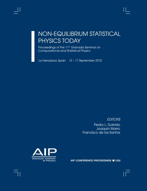
NON-EQUILIBRIUM STATISTICAL<br />
PHYSICS TODAY<br />
Proceedings of the 11 th <strong>Granada</strong> Seminar on<br />
Computational and Statistical Physics<br />
La Herradura, Spain 13 – 17 September 2010<br />
EDITORS<br />
Pedro L. Garrido<br />
Joaquín Marro<br />
Francisco <strong>de</strong> los Santos<br />
AIP CONFERENCE PROCEEDINGS 1332
Garrido<br />
Marro<br />
Santos<br />
NON-EQUILIBRIUM STATISTICAL PHYSICS TODAY 1332
ISBN 978-0-7354-0887-6<br />
ISSN 0094-243X
NON-EQUILIBRIUM STATISTICAL<br />
PHYSICS TODAY<br />
fm_1332.indd 1 3/3/11 12:22:08 AM
To learn more about AIP Conference Proceedings, including the<br />
Conference Proceedings Series, please visit the webpage<br />
http://proceedings.aip.org/proceedings<br />
fm_1332.indd 2 3/3/11 12:22:08 AM
NON-EQUILIBRIUM STATISTICAL<br />
PHYSICS TODAY<br />
Proceedings of the 11 th <strong>Granada</strong> Seminar on<br />
Computational and Statistical Physics<br />
La Herradura, Spain 13 – 17 September 2010<br />
SPONSORING ORGANIZATIONS<br />
Spanish Minister for Science and Technology<br />
Regional Administration “Junta <strong>de</strong> Andalucía”<br />
European Physical Society<br />
Institute “<strong>Carlos</strong> I” for Theoretical and Computational Physics<br />
University of <strong>Granada</strong><br />
All papers have been peer reviewed<br />
EDITORS<br />
Pedro L. Garrido<br />
Joaquín Marro<br />
Francisco <strong>de</strong> los Santos<br />
Melville, New York, 2011<br />
AIP CONFERENCE PROCEEDINGS 1332<br />
fm_1332.indd 3 3/3/11 12:22:08 AM
Editors<br />
Pedro L. Garrido<br />
Joaquín Marro<br />
Francisco <strong>de</strong> los Santos<br />
Institute “<strong>Carlos</strong> I” for Theoretical and Computational Physics<br />
University of <strong>Granada</strong><br />
18071 – <strong>Granada</strong>, Spain<br />
E-mail: garrido@onsager.ugr.es<br />
Authorization to photocopy items for internal or personal use, beyond the free copying permitted<br />
un<strong>de</strong>r the 1978 U.S. Copyright Law (see statement below), is granted by the American Institute<br />
of Physics for users registered with the Copyright Clearance Center (CCC) Transactional<br />
Reporting Service, provi<strong>de</strong>d that the base fee of $30.00 per copy is paid directly to CCC, 222<br />
Rosewood Drive, Danvers, MA 01923, USA. For those organizations that have been granted a<br />
photocopy license by CCC, a separate system of payment has been arranged. The fee co<strong>de</strong> for<br />
users of the Transactional Reporting Services is: 978-0-7354-0887-6/11/$30.00<br />
© 2011 American Institute of Physics<br />
Permission is granted to quote from the AIP Conference Proceedings with the customary<br />
acknowledgment of the source. Republication of an article or portions thereof (e.g., extensive<br />
excerpts, fi gures, tables, etc.) in original form or in translation, as well as other types of reuse<br />
(e.g., in course packs) require formal permission from AIP and may be subject to fees. As a courtesy,<br />
the author of the original proceedings article should be informed of any request for republication/reuse.<br />
Permission may be obtained online using Rightslink. Locate the article online at<br />
http://proceedings.aip.org, then simply click on the Rightslink icon/“Permission for Reuse” link<br />
found in the article abstract. You may also address requests to: AIP Offi ce of Rights and<br />
Permissions, Suite 1NO1, 2 Huntington Quadrangle, Melville, NY 11747-4502, USA; Fax: 516-<br />
576-2450; Tel.: 516-576-2268; E-mail: rights@aip.org.<br />
L.C. Catalog Card No. 2010943018<br />
ISBN 978-0-7354-0887-6<br />
ISSN 0094-243X<br />
Printed in the United States of America<br />
fm_1332.indd 4 3/3/11 12:22:08 AM
AIP Conference Proceedings, Volume 1332<br />
Non-equilibrium Statistical Physics Today<br />
Proceedings of the 11th <strong>Granada</strong> Seminar on Computational and<br />
Statistical Physics<br />
Preface<br />
J. Marro<br />
Table of Contents<br />
Nonequilibrium statistical physics today. Where shall we go from here?<br />
Pedro L. Garrido, Joaquín Marro, Francisco <strong>de</strong> los Santos, and Joel L.<br />
Lebowitz<br />
Three lectures: NEMD, SPAM, and shockwaves<br />
Wm. G. Hoover and Carol G. Hoover<br />
Stochastic thermodynamics: An introduction<br />
Udo Seifert<br />
Hydrodynamics from dynamical non-equilibrium MD<br />
Sergio Orlandini, Simone Meloni, and Giovanni Ciccotti<br />
Recent progress in fluctuation theorems and free energy recovery<br />
A. Alemany, M. Ribezzi, and F. Ritort<br />
Universality in equilibrium and away from it: A personal perspective<br />
Miguel A. Muñoz<br />
Fourier law, phase transitions, and the Stefan problem<br />
Errico Presutti<br />
Bringing thermodynamics to non-equilibrium microscopic processes<br />
J. M. Rubí<br />
Noise-induced transitions vs. noise-induced phase transitions<br />
Raúl Toral<br />
v<br />
1<br />
3<br />
23<br />
56<br />
77<br />
96<br />
111<br />
123<br />
134<br />
145
On the approach to thermal equilibrium of macroscopic quantum<br />
systems<br />
Sheldon Goldstein and Ro<strong>de</strong>rich Tumulka<br />
Temperature, entropy and second law beyond local equilibrium: An<br />
illustration<br />
David Jou<br />
Griffiths phases in the contact process on complex networks<br />
Géza Ódor, Róbert Juhász, Claudio Castellano, and Miguel A. Muñoz<br />
Stationary points approach to thermodynamic phase transitions<br />
Michael Kastner<br />
Energy bursts in vibrated shallow granular systems<br />
N. Rivas, D. Risso, R. Soto, and P. Cor<strong>de</strong>ro<br />
Layering and wetting transitions for an interface mo<strong>de</strong>l<br />
Salvador M. Solé<br />
On the role of Galilean invariance in KPZ<br />
H. S. Wio, J. A. Revelli, C. Escu<strong>de</strong>ro, R. R. Deza, and M. S. <strong>de</strong> La Lama<br />
Anomalous diffusion and basic theorems of statistical mechanics<br />
Luciano C. Lapas, J. M. Rubí, and Fernando A. Oliveira<br />
Large <strong>de</strong>viations of the current in a two-dimensional diffusive system<br />
C. Pérez-Espigares, J.J. <strong>de</strong>l Pozo, P.L. Garrido, and P.I. Hurtado<br />
Stochastic resonance between propagating exten<strong>de</strong>d attractors<br />
M. G. <strong>de</strong>ll'Erba, G. G. Izús, R. R. Deza, and H. S. Wio<br />
Heat and chaotic velocity in special relativity<br />
A. L. Garcia-Perciante<br />
Computing free energy differences using conditioned diffusions<br />
Carsten Hartmann and Juan Latorre<br />
Dynamical behavior of heat conduction in solid Argon<br />
Hi<strong>de</strong>o Kaburaki, Ju Li, Sidney Yip, and Hajime Kimizuka<br />
Fast transients in mesoscopic systems<br />
A. Kalvová, V. Špička, and B. Velický<br />
vi<br />
155<br />
164<br />
172<br />
179<br />
184<br />
190<br />
195<br />
200<br />
204<br />
214<br />
216<br />
218<br />
221<br />
223
Dynamical aspect of group chase and escape<br />
Shigenori Matsumoto, Tomoaki Nogawa, Atsushi Kamimura, Nobuyasu<br />
Ito, and Toru Ohira<br />
Onset of thermal rectification in gra<strong>de</strong>d mass systems: Analysis of the<br />
classic and quantum self-consistent harmonic chain of oscillators<br />
Emmanuel Pereira, Humberto C. Lemos, and Ricardo R. Ávila<br />
Covariant Lyapunov vectors and local exponents<br />
Harald A. Posch and Hadrien Bosetti<br />
Statics and dynamics of a harmonic oscillator coupled to a onedimensional<br />
Ising system<br />
A. Prados, L. L. Bonilla, and A. Carpio<br />
Strong ratchet effects for heterogeneous granular particles in the<br />
Brownian limit<br />
Pascal Viot, Alexis Bur<strong>de</strong>au, and Julian Talbot<br />
Stochastic protein production and time-<strong>de</strong>pen<strong>de</strong>nt current fluctuations<br />
Mieke Gorissen and Carlo Van<strong>de</strong>rzan<strong>de</strong><br />
Creating the conditions of anomalous self-diffusion in a liquid with<br />
molecular dynamics<br />
J. Ryckebusch, S. Standaert, and L. De Cruz<br />
Cluster size distribution in Gaussian glasses<br />
S.V. Novikov<br />
A non-equilibrium potential function to study competition in neural<br />
systems<br />
Jorge F. Mejías<br />
Quasi-stationary states and a classification of the range of pair<br />
interactions<br />
A. Gabrielli, M. Joyce, and B. Marcos<br />
Fluctuation relations and fluctuation-response relations for molecular<br />
motors<br />
G. Verley and D. Lacoste<br />
Why are so many networks disassortative?<br />
Samuel Johnson, Joaquín J. Torres, J. Marro, and Miguel A. Muñoz<br />
vii<br />
226<br />
228<br />
230<br />
232<br />
235<br />
237<br />
239<br />
241<br />
243<br />
245<br />
247<br />
249
Analytical study of hysteresis in the T = 0 random field Ising mo<strong>de</strong>l<br />
T. P. Handford, F-J Perez-Reche, and S N Taraskin<br />
Queues on narrow roads and in airplanes<br />
Vidar Frette and Per C. Hemmer<br />
Fluctuations out of equilibrium<br />
V. V. Belyi<br />
Long-range interacting systems and dynamical phase transitions<br />
Fulvio Baldovin, Enzo Orlandini, and Pierre-Henri Chavanis<br />
Irreversibility of the renormalization group flow and information theory<br />
S. M. Apenko<br />
Classical systems: Moments, continued fractions, long-time<br />
approximations and irreversibility<br />
R. F. Álvarez-Estrada<br />
ABSTRACTS OF SELECTED CONTRIBUTIONS<br />
Reentrant behavior of effective attraction between like-charged<br />
macroions immersed in electrolyte solution<br />
Ryo Akiyama, Ryo Sakata, and Yuji I<strong>de</strong><br />
Nonlinear Boltzmann equation for the homogeneous isotropic case:<br />
Some improvements to <strong>de</strong>terministic methods and applications to<br />
relaxation towards local equilibrium<br />
P. Asinari<br />
Effective dimension in flocking mechanisms<br />
Gabriel Baglietto and Ezequiel V. Albano<br />
The Liouville equation and BBGKY hierarchy for a stochastic particle<br />
system<br />
M. Baryło<br />
To mo<strong>de</strong>l kinetic <strong>de</strong>scription<br />
V.V. Belyi<br />
viii<br />
251<br />
253<br />
255<br />
257<br />
259<br />
261<br />
265<br />
266<br />
267<br />
268<br />
269
Experimental <strong>de</strong>nsities of binary mixtures: Acetic acid with benzene at<br />
several temperatures<br />
Georgiana Bolat, Daniel Sutiman, and Gabriela Lisa<br />
Enhanced memory performance thanks to neural network assortativity<br />
S. <strong>de</strong> Franciscis, S. Johnson, and J. J. Torres<br />
New insights in a 2-D hard disk system un<strong>de</strong>r a temperature gradient<br />
J. J. <strong>de</strong>l Pozo, C. Pérez-Espigares, P.I. Hurtado, and P.L. Garrido<br />
Automatic optimization of experiments with coupled stochastic<br />
resonators<br />
Mauro F. Calabria and Roberto R. Deza<br />
Velocity-velocity correlation function for anomalous diffusion<br />
Rogelma M. Ferreira and Fernando A. Oliveira<br />
Excess of low frequency vibrational mo<strong>de</strong>s, glass transition and inherent<br />
structures<br />
Hugo M. Flores-Ruiz and Gerardo G. Naumis<br />
Analysis of ship maneuvering data from simulators<br />
Vidar Frette, G. Kleppe, and K. Christensen<br />
Unfying approach for fluctuation theorems from joint probability<br />
distributions<br />
Reinaldo García-García, D. Domínguez, Vivien Lecomte, and A.B.<br />
Kolton<br />
Thermally activated escape far from equilibrium: A unified pathintegral<br />
approach<br />
S. Getfert and P. Reimann<br />
The crystal nucleation theory revisited: The case of 2D colloidal crystals<br />
A.E. González and L. Ixtlilco-Cortés<br />
Space-time phase transitions in the totally asymmetric simple exclusion<br />
process<br />
M. Gorissen and C. Van<strong>de</strong>rzan<strong>de</strong><br />
Mo<strong>de</strong>ling of early stages of island growth during pulsed <strong>de</strong>position: Role<br />
of closed compact islands<br />
M. Kotrla and M. Masin<br />
ix<br />
270<br />
271<br />
272<br />
273<br />
274<br />
275<br />
276<br />
277<br />
278<br />
279<br />
280<br />
281
Fluctuations of the dissipated energy in a granular system<br />
Antonio Lasanta, Pablo I. Hurtado, Pedro L. Garrido, and J. J. Brey<br />
Study of the dynamic behavior of quantum cellular automata in<br />
graphane nanoclusters<br />
A. León and M. Pacheco<br />
Breeding gravitational lenses<br />
J. Liesenborgs, S. De Rijcke, H. Dejonghe, and P. Bekaert<br />
Improved macroscopic traffic flow mo<strong>de</strong>l for aggresive drivers<br />
A. R. Mén<strong>de</strong>z and R. M. Velasco<br />
A formula on the pressure for a set of generic points<br />
A.M. Meson and F. Vericat<br />
Statistical thermodynamics of a relativistic gas<br />
Afshin Montakhab and Malihe Ghodrat<br />
Noninteracting classical spins in a rotating magnetic field: Exact results<br />
Suhk K. Oh and Seong-Cho Yu<br />
Optimal mutation rates in dynamic environments: The Eigen mo<strong>de</strong>l<br />
Mark Ancliff and Jeong-Man Park<br />
Current fluctuations in a two dimensional mo<strong>de</strong>l of heat conduction<br />
<strong>Carlos</strong> Pérez-Espigares, Pedro L. Garrido, and Pablo I. Hurtado<br />
Quasistatic heat processes in mesoscopic non-equilibrium systems<br />
J. Pešek and K. Netočný<br />
Violation of fluctuation-dissipation theorem in the off-equilibrium<br />
dynamics of a system with nonadditive interactions<br />
O. A. Pinto, F. Romá, A.J. Ramirez-Pastor, and F. Nieto<br />
Geometric aspects of Schnakenberg's network theory of macroscopic<br />
nonequilibrium observables<br />
M. Polettini<br />
Nonequilibrium thermodynamics of single DNA hairpins in a dual-trap<br />
optical tweezers setup<br />
M. R. Crivellari, J. M. Huguet, and F. Ritort<br />
x<br />
282<br />
283<br />
284<br />
285<br />
286<br />
287<br />
288<br />
289<br />
290<br />
291<br />
292<br />
293<br />
294
Quantum revivals and Zitterwebegung in monolayer graphene<br />
Elvira Romera and Francisco <strong>de</strong> los Santos<br />
The non-equilibrium and energetic cost of sensory adaptation<br />
G. Lan, Pablo Sartori, and Y. Tu<br />
Negative specific heat in the canonical statistical ensemble<br />
F. Staniscia, A. Turchi, D. Fanelli, P.H. Chavanis, and G. De Ninno<br />
Dynamical systems approach to the study of a sociophysics agent-based<br />
mo<strong>de</strong>l<br />
Andrá M. Timpanaro and Carmen P. Prado<br />
Conversion process of chemical reaction into mechanical work through<br />
solvation change<br />
Ken Tokunaga, Takuya Furumi, and Ryo Akiyama<br />
Participants List<br />
Author In<strong>de</strong>x<br />
xi<br />
295<br />
296<br />
297<br />
298<br />
299<br />
301<br />
303
EDITORS' PREFACE<br />
This volume originated at the 11 th <strong>Granada</strong> Seminar organized by the University of<br />
<strong>Granada</strong>, Spain, and contains the main lectures, a transcription of the discussions in an open<br />
round table (of which the book takes its title), and a selection of contributed papers in that<br />
conference. This is the eleventh of a series of <strong>Granada</strong> Lectures previously published by:<br />
World Scientific (Singapore 1993),<br />
Springer Verlag (Lecture Notes in Physics volumes 448 and 493),<br />
Elsevier (Computer Physics Communications volume 121-122), and<br />
American Institute of Physics (Conference Proceedings Series, volumes 574, 661, 779,<br />
887 and 1091).<br />
These books and the successive editions of the Seminar since 1990 are <strong>de</strong>scribed in <strong>de</strong>tail at<br />
http://ergodic.ugr.es/cp/. This web also contains updated information on the next edition.<br />
The <strong>Granada</strong> Seminar is <strong>de</strong>fined as a small topical conference whose pedagogical effort<br />
is especially aimed at young researchers. In fact, one interesting aspect of this meeting is the<br />
opportunity given to the youngest to present their results and to discuss their problems with<br />
leading specialists. There were in this edition a total of 60 lectures and 42 poster contributions.<br />
More than one hundred participants came from nearly thirty countries (Spain contributed with<br />
21%, the rest of Europe including Russia with 48%, North America with 7%, Central and South<br />
America with 15%, Asia with 7%, and Africa with 2%); most of the participants received partial<br />
support from the organization.<br />
The 11 th <strong>Granada</strong> Seminar was organized by the Institute <strong>Carlos</strong> I for Theoretical and<br />
Computational Physics of the University of <strong>Granada</strong>, sponsored by the European Physical<br />
Society, endorsed by The American Physical Society, and financed by the Spanish Minister for<br />
Science, project MICINN FIS2009-08191E, by the regional administration Junta <strong>de</strong> Andalucía,<br />
and by the University of <strong>Granada</strong>. We also wish to express gratitu<strong>de</strong> to all those who have<br />
collaborated in making this event a success. In particular, we mention the remarkably high<br />
quality and friendly cooperation of invited speakers, among which we should distinguish Joel<br />
Lebowitz whose (80+⅓) th anniversary we celebrated during the meeting, and other participants,<br />
whose personal effort enabled us to accomplish the goals of the Seminar, the Steering<br />
Committee's help in <strong>de</strong>signing format and contents, and further in situ collaboration from<br />
colleagues and stu<strong>de</strong>nts. This edition of the Seminar was held from 13 to 17 of September 2010<br />
in the charming village of La Herradura, a remarkable spot of the Tropical Coast of <strong>Granada</strong>,<br />
where the participants enjoyed a paradisiacal setting with excellent hotels and restaurants.<br />
Finally, let us notice that an effort has been ma<strong>de</strong> by authors and editors to offer<br />
pedagogical notes here; in particular, each topic is comprehensively <strong>de</strong>scribed within its<br />
scientific context. We try to mold the <strong>Granada</strong> Lectures into a series of books that help<br />
introduce the beginner to novel advances in statistical physics and to the creative use of<br />
computers in scientific research, as well as to serve as a work of reference for teachers,<br />
stu<strong>de</strong>nts and researchers.<br />
<strong>Granada</strong>, 18 November 2010
GRANADA SEMINAR<br />
STEERING COMMITTEE<br />
K. Bin<strong>de</strong>r, Institute of Physics of Con<strong>de</strong>nsed Matter, University of Mainz<br />
H. J. Herrmann, ICA1, University of Stuttgart<br />
J. L. Lebowitz, Department of Mathematics, Rutgers University, New Jersey<br />
R. <strong>de</strong> la Llave, Department of Mathematics, University of Texas, Austin<br />
M. Mareschal, Faculté <strong>de</strong>s Sciences, Université Libre <strong>de</strong> Bruxelles<br />
J. F. Fernán<strong>de</strong>z, Institute for Materials Science, C.S.I.C. and University of Zaragoza<br />
P. L. Garrido, Institute "<strong>Carlos</strong> I" for Theoretical and Computational Physics,<br />
University of <strong>Granada</strong><br />
H. J. Kappen, Department of Biophysics, University of Nijmegen<br />
J. Marro, Departamento <strong>de</strong> E. y Física <strong>de</strong> la Materia, University of <strong>Granada</strong>
Nonequilibrium Statistical Physics today.<br />
Where shall we go from here?<br />
This is an edited transcription, by Pedro L. Garrido, Joaquín Marro, and Francisco <strong>de</strong> los<br />
Santos, of the directly recor<strong>de</strong>d sound during an open round table, the third day of the Seminar,<br />
which was chaired by Prof. Joel L. Lebowitz. 1<br />
• Joel L. Lebowitz (JLL): This was supposed to be the last sli<strong>de</strong> of my talk on Monday.<br />
. . It will serve here to say what I consi<strong>de</strong>r important open problems in un<strong>de</strong>rstanding<br />
nonequilibrium phenomena. These, I think, are very central issues. . . though not the only<br />
ones.<br />
FIGURE 1. The sli<strong>de</strong> from Lebowitz’s talk (not inclu<strong>de</strong>d in the book) which is often referred to within<br />
the discussions. (NESS stands for Nonequilibrium Steady States.)<br />
The first thing is the free energy for a nonequilibrium stationary state. Consi<strong>de</strong>r a<br />
system in contact with two reservoirs, one temperature on the left, and one temperature<br />
on the right, in a stationary state. Question: is there a reasonable <strong>de</strong>finition of free energy<br />
for such an open nonequilibrium system? In my talk I was saying that if you start a state,<br />
1 The speakers had a chance to swiftly revise the text. The fresh, informal way of talking during the<br />
discussions, and some eventual references ma<strong>de</strong> to the blackboard there have been kept whenever the<br />
meaning is still reasonably evi<strong>de</strong>nt. A few in<strong>de</strong>cipherable sentences have been replaced by [. . . ].
say a temperature profile, then the large <strong>de</strong>viation function will <strong>de</strong>crease to the stationary<br />
one in a monotone way. In other words, the log of the probability of having such a<br />
profile in the stationary state [which is not typical], will as the time evolves (assuming<br />
Fourier’s law is satisfied; we are not talking about anomalous systems here) increase,<br />
with the system eventually coming to the stationary state. I argue that this is analogous<br />
to what you find if you have an isolated macroscopic system with fixed total energy in<br />
a nontypical initial state, then it will eventually come to something that is uniform. So<br />
the final state will be an equilibrium state which, as I argued several times already, is<br />
essentially something which occupies the whole energy surface, but not really the total<br />
full energy surface. There are going to be some regions, more unlikely the larger the<br />
system, this will be exponential with the size of the system. By the way, I’m very much<br />
an individualist that will later ask for someone to <strong>de</strong>fend the ensemblist point of view<br />
that Shelly was saying over there. The microcanonical ensemble gives you a certain<br />
probability, a large <strong>de</strong>viation, and then the second law says that this large <strong>de</strong>viation<br />
function which is the difference between the entropy of the actual macroscopic state,<br />
and the equilibrium entropy, (which is equivalent to the Gibbs entropy of a uniform<br />
distribution over the energy surface when the system is large), is going to be monotone.<br />
If you have the same temperature on the two si<strong>de</strong>s, the stationary state will correspond<br />
to a canonical distribution with this temperature. The energy will no longer be constant<br />
but the system will go to a state with a uniform temperature.<br />
What about a nonequilibrium stationary state, when you actually have transport of<br />
energy along the system? Then, I argue again, the large <strong>de</strong>viation function will be<br />
monotone. This <strong>de</strong>pends on the log of the ratio of the probability of the typical state<br />
to the one you started out with, which is not typical.<br />
In equilibrium, entropy plays more than one role: it is the large <strong>de</strong>viation function but<br />
in addition if you take the <strong>de</strong>rivative of the entropy with respect to the energy you get<br />
one over the temperature, you can get the pressure by taking the <strong>de</strong>rivative of the entropy<br />
with respect to the volume for a given energy, etc. People have tried for many, many<br />
years to find an equivalent thing for this nonequilibrium stationary ensemble. I have<br />
certainly been trying since when I did my thesis, it was before any of you here were born<br />
probably. In 1956 I was trying to find what the analogous thing to the thermodynamic<br />
free energy is in a nonequilibrium stationary state. That problem has not been solved.<br />
In fact I don’t think much progress has been ma<strong>de</strong> on that for the last 60 years. In<br />
particular, Tasaki and his coworkers have tried to <strong>de</strong>velop something, I don’t think very<br />
successfully, maybe there simply isn’t anything like that. It’s an open question.<br />
The second open question is even simpler: it is just to <strong>de</strong>rive macroscopic equations<br />
for realistic Hamiltonian microscopic dynamics. As Roberto [Livi] was saying, let’s say<br />
that equations like Fourier’s law don’t necessarily always hold when you are in low<br />
dimensions (and other things we know don’t hold). But experimentally it seems to be<br />
very, very good for most systems. When you have a metal bar between two temperatures,<br />
or just a metal bar by itself and you start with a nonuniform temperature, Fourier’s law<br />
holds. It would be very, very nice if one could <strong>de</strong>rive that from microscopic dynamics,<br />
classical or quantum mechanical, I mean, quantum mechanical would be even better,<br />
even though I don’t agree at all with Sandu [Popescu] that there is any problem with the<br />
classical un<strong>de</strong>rstanding. In fact I think there are some problems with the quantum thing,<br />
but I’ll come to that later.
The third issue is really, if you wish, a subset of the first one. This is supposed to be<br />
the energy surface. . . This is what I call Γ1. It’s a region on the energy surface, which<br />
corresponds to some particular macrostate at time t1. I’m thinking again of an isolated<br />
system having an energy <strong>de</strong>nsity profile corresponding to a macrostate but which has a<br />
very small volume, it’s very unlikely with respect to the microcanonical ensemble. Then<br />
at time t2 you will get a new macrostate, Γ2, which is going to be, let’s say much more<br />
uniform, and will have a much larger region in the phase space. Now you want to predict<br />
what is going to happen next time, let’s say at time t3. Γ2 will very likely go to a state<br />
M3 of much larger region Γ3.<br />
The point is, let me say it again: To have a <strong>de</strong>terministic macroscopic equation, I<br />
mean that almost all the phase points in the region Γ1 go into Γ2 and the values of<br />
the macrovariables associated to Γ2 are a solution of the <strong>de</strong>terministic equations like<br />
the Fourier Law. You know, the <strong>de</strong>rivative of the energy <strong>de</strong>nsity with respect to time is<br />
given by the divergence of some energy flux, and this energy flux is given by minus the<br />
gradient of temperature. So, if I say I have <strong>de</strong>terministic equations which lead me from<br />
a profile at time t1 to a profile at time t2, according to the solution of the heat equation<br />
for isolated systems, I mean that almost all of the phase points initially in Γ1 end up<br />
in Γ2. By the Liouville theorem, the volume of Γ1 is preserved so the intersection of<br />
the evolved Γ1 and Γ2 will have the same volume, or maybe slightly smaller because<br />
some of the phase points in Γ1 have “leaked out”. So it’s a very, very sparse set. In a<br />
certain respect it’s a very atypical set because if I reverse all the velocities I’ll be going<br />
exactly back over there [Γ1], which is very atypical. Almost any point in Γ2, reversing<br />
the velocities, will go to the bigger set Γ3. Nevertheless, if you are going to have a<br />
<strong>de</strong>terministic time evolution, it must mean that this set over here [U(t2,t1)Γ1], which is<br />
clearly atypical as far as the past time evolution, behaves typically as far as the future<br />
time evolution goes. And this is really the crux of the mathematical problem of <strong>de</strong>riving<br />
<strong>de</strong>terministic macroscopic equations from microscopic dynamics. To show, that the set<br />
[U(t2,t1)Γ1] behaves typically as far as the future goes with respect to all the points in<br />
Γ2.<br />
So, those are the issues I was going to write down at the end of my talk on Monday<br />
which I consi<strong>de</strong>r some of the important problems in nonequilibrium statistical mechanics<br />
from a foundational point of view. Let me stop now and start having some comments<br />
from you.<br />
• Giovanni Ciccotti (GC): I un<strong>de</strong>rstand what you say. However, as you know, the hydrodynamic<br />
equations are closed, because we add to the conservation law the phenomenological<br />
relations that are given by the constitutive equations i.e. empirical relationships.<br />
Therefore, although we can trust them practically, they are not completely<br />
foun<strong>de</strong>d, being phenomenological equations. Correct? Instead, If I can compute this<br />
property by numerical molecular dynamics, by atomistic dynamics, I can check your<br />
ansatz. It seems to me that what one should do is to find the way in which, without assuming<br />
anything for the continuum representation, one computes directly the behavior of<br />
the fields involved by microscopic dynamics, and then one can check your hypothesis. I<br />
think this is possible. There are people doing this and, in<strong>de</strong>ed, they find correspon<strong>de</strong>nce.<br />
I don’t see, instead, your mathematical problem because you want to give a theoretical<br />
foundation to equations which are intrinsically only phenomenological.
• JLL: Equations that are phenomenological presumably are used because they actually<br />
work. So real systems do behave according to those phenomenological equations.<br />
We also believe that liquids are ma<strong>de</strong> up of molecules. These molecules un<strong>de</strong>rgo microscopic<br />
dynamics, so a given microstate of the liquid which is basically un<strong>de</strong>r classical<br />
mechanics would be a state where you have positions and velocities.<br />
• GC: On that we agree completely. Let me try restate my question. I still would like to<br />
un<strong>de</strong>rstand what your mathematical problem is because if you start from phenomenological<br />
equations I think is very difficult to give to them a <strong>de</strong>ep justification because they<br />
are phenomenological, so sometime they are valid and some other time not. . .<br />
• JLL: I’m totally on your si<strong>de</strong>. I do want to un<strong>de</strong>rstand the origin of these phenomenological<br />
equations. And I think that to un<strong>de</strong>rstand the origin I have to go to the microscopic<br />
dynamics.<br />
• GC: Absolutely.<br />
• JLL: That’s what I’m saying. Going back to your simulations, suppose you start from<br />
a non-uniform macrostate, so you pick a random point in this region of the phase space.<br />
You would see it evolving, let’s say to the more uniform. Now you start with something<br />
which is more distorted; you see after a while it goes to the previous initial macrostate.<br />
Assuming you do your molecular dynamics perfectly exact, so you have now a new<br />
point in the phase space which has the property, if you reverse all the velocities it will<br />
go backwards, as compared as if you pick simply a point at random here. You will find<br />
that the reverse of the velocities will still make it go over here. It will not change at all.<br />
• GC: OK.<br />
• JLL: So the point in Γ2 that you get from coming from Γ1 is very different with respect<br />
to velocity reversal from a point you pick at random in Γ2. Nevertheless the system<br />
behaves macroscopically in a similar way in the future, as you can predict phenomenologically<br />
or see in your computer, and that’s what I think to prove mathematically or to<br />
un<strong>de</strong>rstand mathematically is an essential problem.<br />
• GC: Then I totally agree. Your problem is strictly macroscopic. You start from the<br />
phenomenological equations when you find that they are satisfied. Why is this, it is not<br />
your problem. Fine.<br />
• Lev Shchur (LS): I don’t completely agree with you that it is possible to check in<br />
molecular dynamics with any precision. Typically, in the picture you showed us, you<br />
have some typical time scale, and Lyapunov exponents. Suppose you can make several<br />
mappings of such a kind but at some point you really forgot the initial one because<br />
you need some exponential precision for that. You know, your <strong>de</strong>rivatives should be<br />
exponentially fine in a way.<br />
• JLL: I don’t think Giovanni says that you can do it experimentally, with infinite<br />
precision. But at least in some simulations we have done on integer arithmetic we did<br />
not have that problem, and still have the same answer. And, after all, the real system,<br />
presumably, to the extent that you can make it isolated, which again is not perfect, you<br />
cannot make it isolated, but I don’t think anyone here doubts that if you make a truly<br />
isolated system and you did truly infinitely precise molecular dynamics, that you would<br />
get any different answer.<br />
• LS: Yes, because in your picture you have Lyapunov exponent which is somehow connected<br />
with the Kolmogorov-Sinai entropy, which is a different entropy which characterizes<br />
the topology of your domains. What is not un<strong>de</strong>rstandable also from your lecture,
is which domain you keep in your mind. Maybe you speak about some special domain<br />
on which you <strong>de</strong>fine your system.<br />
• JLL: Let’s say for the simplest case I would think of a hard sphere system, one with<br />
a Lennard-Jones potential in a given box, conceptually totally isolated, with reflecting<br />
boundary conditions. That’s what I have in mind. As far as one un<strong>de</strong>rstands, at least in<br />
certain regimes, the phenomenological equations would be just absolutely well.<br />
• Miguel Rubí (MR): I want to make a comment on the first point. The question you<br />
raised is very important, to know un<strong>de</strong>r what conditions concepts introduced for systems<br />
in equilibrium such as entropy, free energy or temperature, can also be used in systems<br />
away from equilibrium. I think that this is a crucial point. In my opinion, this question is<br />
very much related to the nature of the noise present in the system. The nature of the noise<br />
may sometimes justify or invalidate the use of equilibrium concepts in non-equilibrium<br />
situations. So, for the particular case of a Gaussian noise, which is common to many<br />
physical systems, one can extend the use of some of these concepts. When the noise<br />
is Gaussian, the stochastic variables vary in a small amount for short time intervals, so<br />
the process is very slow and the probability distribution un<strong>de</strong>rgoes a diffusion processes<br />
governed by a Fokker-Planck equation which is simply a diffusion equation, linear in the<br />
probability. In these cases you can establish a connection with the second law and use<br />
the concept of entropy. However, if the noise is not Gaussian one has to use other kinetic<br />
equations the form of which is different from a diffusion equation. In these cases there<br />
is not a clear connection between the dynamics and the second law. To obtain an entropy<br />
functional compatible with these kinetic equations is not obvious. An example is the<br />
case of a multiplicative noise or other noises such as Poisson or Shot noises. When the<br />
distribution function is non-Gaussian, we do not know how to <strong>de</strong>fine the temperature.<br />
Sometimes, one may <strong>de</strong>fine effective temperatures but these quantities are not robust,<br />
they <strong>de</strong>pend on the particular situation you are consi<strong>de</strong>ring, on the observables and the<br />
initial conditions. These temperatures are not temperatures in a thermodynamic sense.<br />
When the noise is Gaussian the temperature inferred from the variance of the distribution<br />
coinci<strong>de</strong>s with the thermodynamic temperature and everything fits perfectly well. I want<br />
to make a comment on the distinction between the Gaussian nature of the noise and the<br />
Gaussian form of the probability distribution function. In the example I discussed in my<br />
talk on the Brownian motion in a shear-flow, in a stationary flow, the noise is Gaussian<br />
because the particle is immersed in a heat bath. But if you solve the Smoluchowski<br />
equation for a nonlinear velocity profile, for example a Poiseuille flow, you don’t get a<br />
Gaussian form. A Gaussian noise for which the kinetic equation is of the Fokker-Planck<br />
type does not necessarily imply that the probability distribution be a Gaussian. In the<br />
case of a gentle Poisseuille flow in which the system is not far from equilibrium this<br />
distribution function is non-Gaussian. Since the noise is Gaussian you can establish a<br />
connection with the second law and use the concept of entropy. So I insist in the fact that<br />
the nature of the noise is a crucial point in establishing the link between thermodynamics<br />
and stochasticity.<br />
• JLL: You are talking about noise. Presumably, this noise you expect is really internal.<br />
I mean, you don’t think the system would behave differently if it was truly isolated<br />
and followed the laws of the dynamics of classical mechanics. Whatever noise comes<br />
out, I mean, from the dynamics. Of course you don’t want to follow the molecules, you<br />
substitute, you replace it by some kind of noise. But I’m asking the questions at a more
conceptual level. There still will be, I expect, a stationary state but you have the two<br />
different temperatures, insi<strong>de</strong> I take it to be just real dynamics. I’m not pretending I can<br />
solve it, but there is going to be, you know, such a state and I ask, yes it’s a question and<br />
I don’t know the answer. In some cases one can approximate it well enough by means<br />
of some kind of Gaussian distribution and have a kind of thermodynamic local thermal<br />
equilibrium. In other cases you may not, and I think that’s quite likely to be the right<br />
answer.<br />
• MR: The theory of stochastic processes is very useful because if you know the form<br />
of the kinetic equations you can <strong>de</strong>termine the stochastic dynamics of the system, you<br />
can calculate the correlation functions which are related to physical quantities one can<br />
measure. Then you can establish the link between the second law and the stochastic<br />
behavior of the system. In my opinion this is an important point.<br />
• JLL: I am not really worried about the second law. I think the second law can take<br />
care of itself. It is going to do all right. What these people are saying they would like<br />
to have a formalism which is analogous in some sense to the equilibrium formalism<br />
and have some function, in particular Tasaki and his group they say, even if you are in<br />
local equilibrium of course you still have a current flowing so they want to add to the<br />
thermodynamic variables, a local energy <strong>de</strong>nsity, local particle <strong>de</strong>nsity, local velocity,<br />
. . . They want to add a current as a hydrodynamic, as a macroscopic thermodynamic<br />
variable, to find a function of these, including the current as a parameter which would<br />
somehow play a role like free energy in equilibrium. If you differentiate it, you get the<br />
specific heat or you get some other things. I mean, that sort of conceptual question. . . I<br />
think it’s important but probably doesn’t have a unique answer. Equilibrium is probably,<br />
really a special case, it’s a very unique case. When you are not in equilibrium you don’t<br />
have any such universal type of things.<br />
• Sandu Popescu (SP): So, coming to your first thing, to the point with all the molecules<br />
starting in a corner, then they expand through the box and you reach a point that is not<br />
critical towards the future, it behaves as any other typical point. I just want to mention<br />
that, just a comment, that in fact any initial condition is not typical if you <strong>de</strong>fine it in<br />
a precise way. So suppose you have a situation in which the molecules are uniformly<br />
distributed, but you say, well, this is a particular one in which molecule number one is<br />
here, molecule number two is there, so it is very non-typical. Let it evolve and you say<br />
if I would reverse all the velocities will come back to precisely this point. Most of the<br />
others will not do that, but towards the future they all behave the same. So every single<br />
initial condition gives rise to a non-typical case.<br />
• JLL: Yes, sure. What I’m saying here is on the macroscopic level. [. . . ] I get back<br />
maybe to typicality, what do you mean by typical, Shelly [Goldstein]? I think we give<br />
it in our paper. Or not? Take the unit interval, from zero to one. Everyone knows that if<br />
you take Lebesgue measure all the rational points have measure zero. So every rational<br />
point is atypical. Nevertheless, there are certain theorems about typical points. Almost<br />
all points with respect to Lebesgue measure are so called normal. This means that in<br />
any expansion –<strong>de</strong>cimal expansion or binary expansion– the fraction of times I see<br />
in <strong>de</strong>cimal expansions a seven to occur is exactly one tenth of the time, so fraction<br />
of times that 693 appears is exactly one thousand of the times. That’s normal, that’s<br />
a theorem. For almost all numbers, “almost all” meaning with respect to Lebesgue<br />
measure,. . . almost all numbers are normal. Obviously, no rational number satisfies that.
Still, if I give you a number, pick 677000 at random, random in the usual sense, for the<br />
numerator and a similar type of number for the <strong>de</strong>nominator, and I ask you if I make<br />
an expansion, and go up to 500000 <strong>de</strong>cimal places, am I likely to find equal number of<br />
sevens and equal number of eights? You would say, unless you really pick your number<br />
very specially, “I expect that”. So in that sense I think of typical over here. [somebody<br />
interrupts, almost inaudible] Shelly was saying that. . . almost all the energy, here is your<br />
whole energy surface and almost all of it, I mean, really almost all of it, except up to a<br />
tenth to the minus 20 corresponds to equilibrium. No, he doesn’t disagree with that, I<br />
don’t think at all.<br />
• SP: I would actually disagree with you. From your point of view, you see, there is a<br />
conflict in what you say because, on one hand, you would like to <strong>de</strong>fine a point of being<br />
typical just by [. . . ] looking at macroscopic conditions. But if you would be able to view<br />
with infinite precision, then every point would be atypical in some sense towards the<br />
past. But they are all typical towards the future.<br />
• JLL: I don’t think so. I think that in Classical Mechanics and in Quantum Mechanics,<br />
whatever you said for the fraction of time, going from zero to infinity, in an isolated<br />
system I could just as well go from zero to minus infinity and arrive exactly at the<br />
same theorem. As long as the system stays isolated, of course. Why then do we see<br />
this irreversibility in life, in nature? I think that really goes back, you have to go back<br />
to initial conditions. Feynman emphasizes it, and Boltzmann already said it. I forgot<br />
now the exact phrasing of Boltzmann but something when he answers Zermelo. When<br />
Zermelo said, you know, that you have eventually Poincare recurrence, and things like<br />
that. Boltzmann said that what is important to realize is that the behavior of systems is<br />
not <strong>de</strong>termined by dynamics alone. It also involves initial conditions. That’s very crucial.<br />
The dynamics are time symmetric. It’s initial conditions which are not time symmetric.<br />
But if you simply look at the dynamics and pick a point, it is going to be time symmetric.<br />
Is what Shelly was saying, and von Neumann. [. . . ] In reality we don’t see that because<br />
of the initial conditions. Sometimes I have this picture from Roger Penrose where there<br />
is the good lord creating the universe and pointing to some very, very little macrostate<br />
over there. Again, I point to Boltzmann saying in a different way the important part: you<br />
do not have to take a particular microscopic state.<br />
• Roberto Livi (RL): I want to add some comment about what Joel was discussing<br />
before. Well, on the concept of reversibility and trajectories and so on. These are quite<br />
troublesome arguments, but let me give you a piece of information that I know for sure<br />
because I published a paper on this fact. [laughs] These are not just conjectures, these<br />
are results. Take that stuff and put it in contact with two heat baths. With two heat<br />
baths, I mean, the chain I was showing you before. And take it a harmonic chain. Joel<br />
solved that problem many years ago with Rie<strong>de</strong>r and Lieb, and you can work out an<br />
analytical collection, and you know everything about that. In that case you are in a very<br />
anomalous situation. Everybody knows that, you know it follows that [. . . ] there is no<br />
Fourier law, there is nothing about that. But now suppose that you add, and this comes<br />
again as an example of a special kind of noise, a martingale process, which amounts to<br />
add randomly collisions that preserve energy and momentum. So you have the dynamics<br />
but sometimes a couple of particles colli<strong>de</strong>. This can be worked out very easily. [. . . ] The<br />
very important point is that you can compute analytically everything of this problem and<br />
you can compute the nonequilibrium invariant measure. Compute means with analytic
formula, without any approximation or integration scheme. And then you find a very<br />
nice expression, and you find everything that you need to know about this state. The<br />
correlations, spatial correlations appear, you have local thermal equilibrium with the<br />
exception that the tails of these Gaussian distributions certainly have to feel the effect<br />
that you are not in an equilibrium state, so that these tails maintain this memory effect.<br />
So everything here is analytical. Now you take any other mo<strong>de</strong>l, for instance the FPU<br />
mo<strong>de</strong>l or any other kind of nonlinear chain, and then in that case your covariance matrix<br />
can be solved numerically, obviously. And then you apply standard molecular dynamics<br />
method. What do you find? Something which in practice is completely in agreement<br />
with the previous analytical solution, concerning the main ingredients. I’m not saying<br />
the same mo<strong>de</strong>l but the ingredients. The <strong>de</strong>scription of this out of equilibrium stationary<br />
measure obtained by the eigenvalues and eigenvectors of this covariance matrix behave<br />
very gently and very close to what you have observed in the analytic solution of that<br />
problem. So it seems that, for any practical purpose, you obtain what you expect to<br />
obtain <strong>de</strong>spite you have a finite system, <strong>de</strong>spite you have round off errors in your<br />
computation and so on and so forth. And even if you have a small system, this works<br />
perfectly. Obviously, as I was saying before in my talk, you must take care if you want<br />
to exploit numerical simulations to integrate things you don’t know how to integrate in<br />
any other way, you must be very careful in or<strong>de</strong>r to control any finite size effect, any<br />
time length effect and so on and so forth in measuring this covariance matrix elements.<br />
But once you have done that, I mean, you will know also when this will be violated.<br />
You can really predict it on the basis of analytic argument that if you go too far away<br />
in computing these correlations, you lose the information that you want. And in some<br />
sense this goes back to the fact that if you look at these things in a finite time, there<br />
is a typical finite time which is related to the finite length of the system, but once you<br />
have taken that into account the thermodynamic limit problem does not enter the game.<br />
Now, in any numerical simulation, on the other hand, you know that you have round<br />
off errors. And this will affect how the information propagates. There is no way out of<br />
that. Irreversibility in this kind of simulations doesn’t exist because if you reverse your<br />
process you don’t go back to the initial state.<br />
• JLL: You mean of integer matrix?<br />
• RL: In the case of integer matrix I agree, you can do it. But in that case there are other<br />
technical problems that you have to take into account in or<strong>de</strong>r to say over which time<br />
scale you can trust what you observe. [somebody intervenes. Inaudible]<br />
• RL: Yes, I agree. Absolutely if you control and you increase your numerical precision<br />
register to 256 or 512 bits. This is your job at the very end. So, I mean, you make it<br />
correctly. I don’t know if this is sort of miracle, but things work. That’s what I can say,<br />
no more.<br />
• William G. Hoover (WGH): [Going back to Joel’s statements at the beginning] Number<br />
three of your statements looks to me very difficult in<strong>de</strong>ed, but I have a few remarks<br />
on the first two. It seems to me that Helmholtz’ free energy and entropy are not interesting<br />
variables away from equilibrium. Certainly they are in the equilibrium case. But it<br />
seems to me from our experience in simulations that kinetic temperature is a perfectly<br />
good variable away from equilibrium. And it seems to me that if you are interested in<br />
constitutive relations you could start out by thinking of the energy and the kinetic temperature<br />
rather than free energy and entropy. Similarly, there are perfectly good expres-
sions from kinetic theory, even at high <strong>de</strong>nsity, for the heat flux vector and the pressure<br />
tensor. So, as long as you are not too fussy about where these quantities are localized,<br />
everybody agrees on how to calculate the momentum flux and the energy flux. Now, if<br />
you would like to <strong>de</strong>fine those things at points, and in particular if you would like to<br />
<strong>de</strong>fine them at points in such a way that you have spatial <strong>de</strong>rivatives that are continuous<br />
everywhere, you can do this by introducing Lucy’s or Monaghan’s smooth-particle<br />
weight functions, which <strong>de</strong>scribe the contributions of each particle in space. And if you<br />
do that, which Carol [Hoover] will be talking about tomorrow, you will find that the<br />
pressure tensor at a point and the heat flux vector at a point <strong>de</strong>pend on the <strong>de</strong>tails of the<br />
weight function. To me, instead of looking at this as disastrous, it’s actually an opportunity,<br />
in the sense that you can ask yourself which weight function gives the simplest<br />
macroscopic <strong>de</strong>scription.<br />
• JLL: When you say wave function, you mean you are talking Quantum Mechanics or<br />
not?<br />
• WGH: Weight function, not wave function! It’s simply the i<strong>de</strong>a that the influence of<br />
each particle on the nearby <strong>de</strong>nsity is not represented by a <strong>de</strong>lta function but instead by<br />
something like a Gaussian, but compact, with a range of perhaps two or three particle<br />
diameters. Then the fluctuations in the macroscopic <strong>de</strong>scription are small with respect<br />
to one percent in a homogeneous fluid. That’s a very easy thing to do. Carol [Hoover]<br />
will be talking about this tomorrow.<br />
• JLL: May I just summarize what you said? You are saying that even if you don’t have<br />
a free energy or a distribution function like a Gibbs distribution for the stationary state,<br />
things are not so bad. You can get along with that. Go ahead. I just wanted to summarize<br />
what you have said.<br />
• WGH: You are right, and I just wanted to say one other thing regarding numerical<br />
simulations of a stationary state. There is always some kind of thermostat, so we would<br />
have a cold one at the left hand si<strong>de</strong> and a hot one at the right hand si<strong>de</strong>, for instance.<br />
You can calculate, as long as the thermostats are <strong>de</strong>terministic, the Lyapunov spectrum,<br />
so you can see what happens to Gibbs’ entropy as time goes on. After a while, when<br />
one achieves a nonequilibrium steady state, one finds the interesting news that Gibbs’<br />
entropy is diverging to minus infinity, because the system is collapsing onto a [multi]<br />
fractal attractor. In an example that I’ll show tomorrow, the change in the dimensionality<br />
of the steady state with 32 particles is about ten percent. So, instead of having a 192dimensional<br />
distribution like Gibbs’, the distribution is somewhere between 170 and<br />
180 dimensional. So, if you try to take the logarithm of that fractal distribution, it will<br />
diverge. So that is the physical-conceptual basis of my talk, that the kinetic temperature<br />
tensor is a better thing to look at than entropy.<br />
• JLL: We will wait for your talk tomorrow but another discussion, you know, I mean, if<br />
you use different reservoirs like the one that Roberto was talking about, Langevin type of<br />
thing, then you don’t get any such collapse. But again, as you are saying, the properties<br />
of the system that you are interested in are exactly the same more or less, because we<br />
believe, I think it’s correct, I think that Giovanni [Gallavotti] quoted it from 1959, that<br />
the boundary conditions really should not affect what happens.<br />
• GC: Joel, I’d like to add something to this point, and is that to do statistical mechanics<br />
you need an invariant measure, an invariant measure with time, and you find that<br />
this problem of the <strong>de</strong>grees in dimension, if you use the Lebesgue measurement, but
the Lebesgue measurement with the dynamics associated to something like the Nosé-<br />
Hoover thermostat, is no more invariant. So I think this is a question really to be clarified,<br />
it is not at all evi<strong>de</strong>nt that the statistical measurement that you use when you use non<br />
Hamiltonian dynamics is a Lebesgue one. I would take this as possible. . .<br />
• JLL: I agree with that. Maybe let’s hear from some other people.<br />
• Vaclav Spicka (VS): I would like to comment on Joel’s first statements. So, maybe<br />
this <strong>de</strong>rivation of macroscopic equations, I would say that this is the general problem of<br />
correlations between particles, I mean, a many body problem because I’m starting from<br />
some many body problem, I’m writing microscopic equations and then, as everybody<br />
knows, you must do approximations to come out with some macroscopic equation. So,<br />
I’m leaving out some interactions and so on. I’m emerging with irreversible macroscopic<br />
equations. Another addition is that I must <strong>de</strong>fine some initial conditions for this. This is<br />
another tricky point because when I’m <strong>de</strong>fining initial conditions I must somehow know<br />
the history of the system. Because then I don’t know how from scratch what means initial<br />
condition and how I neglect or not neglect correlations. So, basically this is tricky and<br />
as soon as I will <strong>de</strong>rive so-called such equations I must compare this with experiment<br />
because I have no other chance basically. So, I must do this because every time I’m<br />
forced to do approximations and irreversibility is emerging as like something like effect<br />
of approximations, in fact.<br />
• JLL: Maybe you do approximations. I do not know that a metal bar does any approximations.<br />
I know perfectly well what I mean when I start with a metal bar with<br />
some temperature profile and it evolves according to the heat equation. I do not think the<br />
metal bar knows about your approximations.<br />
• VS: But the problem is a realistic Hamiltonian. Because realistic Hamiltonian inclu<strong>de</strong>s<br />
all these interactions and so on.<br />
• JLL: Of course.<br />
• VS: Then I am in trouble with these things and, moreover, I would say that when I<br />
<strong>de</strong>rive some kind of equations from i<strong>de</strong>al <strong>de</strong>nsity matrix or Green functions or, there are<br />
many methods, then in fact I have some clue how to calculate observables. And then<br />
I basically don’t care about any free energy or entropy. So basically, I’m in complete<br />
nonequilibrium state, maybe, it <strong>de</strong>pends basically on time scales and interactions in the<br />
system. If some steady state emerges or not, if free energy is good <strong>de</strong>scription or not,<br />
it <strong>de</strong>pends. . . Basically, this is question of how far I want to generalize thermodynamics<br />
and if it is reasonable to generalize it. . .<br />
• JLL: I think. . . You talked both about my first and second points. [. . . ] What I wrote<br />
down was just the heat equation. I give you an energy profile, say for a metal bar, a<br />
copper bar, and I look how it changes with time, and I find very accurately, maybe not<br />
absolutely perfectly, that it satisfies the Fourier’s law, its equation. And that’s what I<br />
would like to <strong>de</strong>rive, if it is possible to do it, I mean, mathematically, we certainly have<br />
not succee<strong>de</strong>d so far. So it’s an open problem. We have not succee<strong>de</strong>d but we tried.<br />
• JLL: Younger people should speak up. Where are the young people?<br />
• Afshin Montakhab (AM): I’m not sure that I qualify as a young person but at the risk<br />
of not being invited here again I would do the following comment from the information<br />
theoretic point of view. I hold the view that if we had as human beings <strong>de</strong>vices that<br />
actually measured with infinite precision the positions of the particles, or the initial<br />
state of constituents of macroscopic systems with infinite precision, that we measured
the forces between them, then we would never need thermodynamics. We would not<br />
be talking about things like entropy or anything. So, since uncertainty is a part of our<br />
existence, then there is such a thing called entropy, which is the Shannon entropy. And<br />
from the uncertainty or the measure of which is entropy you can actually calculate<br />
quantities that an observer would make, a macroscopic observer with a thermometer,<br />
a barometer and these kind of <strong>de</strong>vices that we normally have in our laboratory, would<br />
make. So I can hold the view that perhaps trying to <strong>de</strong>rive thermodynamics from<br />
Newtonian dynamics is a bit misgui<strong>de</strong>d either you have to make approximations, like<br />
Boltzmann ma<strong>de</strong>, and you don’t really know where the irreversibility comes from. So I<br />
think these two points are divorced from each other. Either you have precision, exact<br />
precision, in which you can actually answer all kinds of questions you ask, or you<br />
don’t. And the fact is we don’t have those precisions. Therefore we have to <strong>de</strong>al with<br />
thermodynamics. And that’s all I want to say. Just as a comment.<br />
• JLL: I would say I would strongly disagree philosophically and conceptually with that<br />
point of view. I mean, do you think if I knew exactly the positions and velocities of all<br />
the molecules in the water, and I put in this thermometer I would get a different answer<br />
than what I get when I don’t know?<br />
• AM: Thermometer is a macroscopic. . .<br />
• JLL: Yes, so supposing I know all the atoms and molecules of the water and of the<br />
thermometer, would I get a different reading than I get. . . ?<br />
• AM: No, no; you wouldn’t, but the point is you don’t have that. That’s impossible.<br />
• JLL: Who cares? I mean, I think it’s a conceptual thing. I never know, nobody knows,<br />
what π is exactly, the number π. You can approximate it up to <strong>de</strong>cimals; does that mean<br />
that π does not exist as a number?<br />
• AM: Yeah, but that’s mathematics, it’s a little bit different from physical reality.<br />
• JLL: I think we have a disagreement there. Many people take the point of view. . . like<br />
Roberto. . . I have written an article too with Christian Maes. It’s about this man who is<br />
a very good man, who dies and goes up to heaven and he meets an angel there, and the<br />
angel has a big bowl filled with hard spheres. And the guy asks: Do you know every<br />
position and velocity? The angel says yes. Then the guy asks, what is the entropy of this<br />
system, the thermodynamic entropy?<br />
• AM: It’s zero.<br />
• JLL: Our answer is that it is exactly the same for the angel and us. Does it make any<br />
difference at all as whether you know them or not? The behavior that we have discussed<br />
is the same. So, my own feeling is that information theory is very, very useful but I<br />
don’t think it really should be part of the foundations or of these questions, where it is<br />
irrelevant.<br />
• AM: I would just say the angel would say entropy is zero. Entropy is zero, you have<br />
everything you need to have, therefore you can answer all kind of questions. Once you<br />
have the dynamic questions you can answer any question.<br />
• JLL: Sure, you can answer any questions but that doesn’t mean entropy is zero because<br />
you can answer all the questions. It is still true that if you start with one part hot and the<br />
other part cold, heat will go from the hot to the cold, and as you know, entropy <strong>de</strong>scribes<br />
that evolution of going from hot to cold but it doesn’t change at all that angel knows<br />
everything.<br />
• AM: OK. Don’t use this against me and invite me again [laughs].
• Matteo Polettini (MP): I do qualify as a young one, but I’m not really expert on<br />
the arguments. . . I do like the point of view of the information theoretic, but I think<br />
that there’s a little bit problem, is entropic, it’s an anthropic reasoning. It puts man on<br />
a special footing and you say, of course, thermalization occurs in any case but [âòe]<br />
in any case we are always talking about a piece of the universe, a system, which will<br />
never be isolated from the rest of the universe. So, when we reason about reversible,<br />
Newtonian equations what we are really talking about is the universe itself. It’s a sort of<br />
cosmological problem. And my question is, does it make sense to <strong>de</strong>rive macroscopic<br />
thermodynamics from microscopic dynamics without worrying about the universe on<br />
the whole? The universe has a peculiar behavior, for example, it’s expanding so things<br />
in the universe are diluting and this might be one of the mechanisms for equilibration.<br />
• JLL: I agree totally with you about non-isolation in practice, but do you think really<br />
the Navier-Stokes equations <strong>de</strong>pend on having non-isolation? I don’t think so. I think it<br />
is true that you don’t have isolation but I think the behavior of diffusion equation will<br />
not be affected if you really had the isolated system. That’s what I would think. That’s<br />
my answer.<br />
• AM: I wanted to make a comment about the comment you ma<strong>de</strong> about the observer.<br />
That’s the same question Joel respon<strong>de</strong>d when I asked the question about the observer<br />
the other day and is that, is the observer a Ph.D. stu<strong>de</strong>nt? The answer to the question is we<br />
have observers in most physics theories; we have an observer in Quantum Mechanics;<br />
we have an observer in special relativity; we have observers in thermodynamics. An<br />
observer in thermodynamics is a <strong>de</strong>vice that has a thermometer, a barometer or whatever,<br />
you know, can just do the experiments and measure quantities that are relevant. So that’s<br />
the observer, it’s not me or you, or a given person’s uncertainty.<br />
• JLL: I believe that there is an objective world which behaves totally the same whether<br />
anybody has precise knowledge of it or not. The universe does not <strong>de</strong>pend on observations.<br />
The laws of motion were always there, we don’t know them exactly, they were<br />
there before there were thermometers, before there were dinosaurs. . .<br />
• AM: What about Quantum Mechanics?<br />
• JLL: Just the same. I think we should go, maybe let Shelly answer that.<br />
• AM: Special relativity? I mean, physical theories always have observables.<br />
• JLL: No, no. I totally disagree with you.<br />
• AM: Maybe we should shut up this.<br />
• André Timpanaro (AT): I would like to just make a comment on this discussion about<br />
what I un<strong>de</strong>rstand as Shannon entropy and what I un<strong>de</strong>rstand as thermodynamic entropy.<br />
Thermodynamic entropy is a kind of Shannon entropy when your only information are<br />
the thermodynamic variables. Suppose you have a gas. The entropy <strong>de</strong>pends on the temperature,<br />
the pressure and the volume. So the thermodynamic entropy of that gas is the<br />
Shannon entropy that you would have if you only had those three informations. Suppose<br />
then you expand your gas, you make a free expansion, the thermodynamic entropy would<br />
increase but the Shannon entropy remains the same. The previous temperature, pressure<br />
and volume are still the same. Now, if you had a new box with the same macroscopic<br />
variables than the expan<strong>de</strong>d box, then you can’t say about it the same things you could<br />
about the first box, because its Shannon entropy is bigger, it is the new thermodynamic<br />
entropy.
• JLL: I think in general. . . What I call the Boltzmann entropy, logarithm of the macroscopic<br />
phase coinci<strong>de</strong>s with your Shannon entropy when your system is in equilibrium.<br />
If it is in equilibrium it coinci<strong>de</strong>s. It does not coinci<strong>de</strong>, as you pointed out, when you<br />
go out of equilibrium because the Shannon entropy will not change with time, well the<br />
thermodynamic entropy and the Boltzmann entropy will. I don’t think there is any contradiction<br />
there.<br />
• AT: But suppose I got the expan<strong>de</strong>d box and showed it to you. If I ask you what the<br />
Shannon entropy is, you’ll tell me it’s the thermodynamic entropy. You don’t know what<br />
the three macroscopic variables were before expanding the box, so you can’t say the<br />
same things I can say about it.<br />
• JLL: No, for me thermodynamic entropy is what the thermodynamic entropy is. And<br />
if it happens to coinci<strong>de</strong> with the Shannon’s, fine.<br />
• SP: If you allow me to just to make one more comment regarding to this discussion.<br />
I think that the main point is the following. Obviously if you know the position and<br />
velocity of every single molecule in the gas, or in your cup of coffee, will not change<br />
the fact that if you put a thermometer will show the same thing. And that heat goes from<br />
the cold to the hot and so on, well the other way around. So, from that point of view is<br />
good to still continue and have the same notion of entropy because that allows you to<br />
answer all these questions. But the point is that if you actually know the positions and<br />
the velocities, there are new things that you can do. So, for the old thing of putting the<br />
thermometer is the same. But now, if you know. . . , now you can actually extract work<br />
of that thing because you can put mirrors. . . So, it is this difference, that now you can<br />
do other things, that previously you couldn’t do. And for this is good to have a different<br />
notion of entropy that will reflect that.<br />
• JLL: I think I would not disagree that you can do more things if you know more.<br />
I think I would not disagree with that. You can have many, many notions of entropy.<br />
As I mentioned, the Shannon entropy was called entropy, at least according to legend,<br />
because von Neumann said to Shannon “if you call it entropy then it has a resonance, and<br />
then since nobody knows what entropy is nobody can argue with you”. I should mention<br />
just one relevant fact. I showed in my talk on Monday a quotation from Thomson which<br />
I think was the first to clearly raise the question that, if you reverse all the velocities,<br />
everything would go in the other way. Then you go down to say that, an actual fact,<br />
because our sensitivity to initial conditions or perturbations. . . if you really try to . . . you<br />
can make any error, any even slight error in reversing the velocities, you will find that it<br />
behaves just as you expected to behave before. Because any imprecision will lead you<br />
again to, say, the bigger region of the phase space. In or<strong>de</strong>r to get into a very small region<br />
you have to be infinitely or very, very precise. The more chaotic the dynamics and the<br />
larger the number of particles, the more precise. To get out from the small region into<br />
the big region you don’t have to be very precise. That answers also the question: why<br />
doesn’t the noise make a big difference? Because if you are going in the direction of the<br />
expanding phase space volume, we would expect if you make a small perturbation it is<br />
not going to change that. However if you are going into something very, very small, any<br />
small perturbation is going to make an effect. It’s like, you know, the situation if you try<br />
to park a car in a very tight space or get out from a very tight space. It is not at all the<br />
same effort. I mean, it is much easier to get out because there is much, much more space<br />
there, so a small error doesn’t matter but getting in you are going to scrape your car on
your neighbor’s car if you are not infinitely precise.<br />
• Harald Posch (HP): I think one can view these things by looking at the blackboard.<br />
The picture you draw there is a bit misleading. You start out with a little blob in phase<br />
space, which presumes that you have a partition in phase space. Then take a little volume.<br />
If we evolve this little blob forward in time, then we know what will happen: the system,<br />
let’s assume it is isolated, will change such that the volume is conserved, and we’ll get a<br />
very fine filament all over the whole phase space. What counts is what Kolmogorov<br />
called mixing in phase space. That’s the key quantity. And this is measured by the<br />
Kolmogorov-Sinai entropy. So the Kolmogorov-Sinai entropy is the key question. If<br />
we compare now the original blob with the filamented situation at a later time, most of<br />
the measure will be spread out over the whole phase space, and only a small part of<br />
it will have remained in the volume of our original blob. When we do a measurement<br />
we are necessarily forced to project down onto such a partition. So, if you put your<br />
thermometer in, it will not be infinitely thin. The projection introduces irreversibility<br />
into this problem.<br />
• JLL: So you think an isolated system following Newtonian laws will not behave in<br />
the way I said?<br />
• HP: No, no. I just wanted to build the bridge between these various view points.<br />
• JLL: Oh, yeah, I think I un<strong>de</strong>rstand what you are saying and think that it is absolutely<br />
correct, I would agree. That is,. . . things are really much more mixed up over there and,<br />
therefore, <strong>de</strong>spite the fact that they are very atypical, this is a very specific thing [. . . ]. I<br />
agree with that. That’s really a mathematical question, to be able to show, to prove that<br />
is central. I mean, I think we agree entirely. The reason is in<strong>de</strong>ed conceptual; this is very,<br />
very mixed up over there. Yeah.<br />
• HP: If one takes this into account, I mean, then all these different view points can be<br />
seen on the same level, and we do not have difficulties, going from one picture to the<br />
other.<br />
• JLL: I agree. There is only one true picture for a system evolving in time.<br />
• Errico Presutti (EP): It’s a very short comment. I want to say that von Neumann was<br />
terribly wrong, because we don’t know anything about it, but we have been arguing a<br />
lot.<br />
• JLL: So, why was he wrong, in what way?<br />
• EP: Because he says nobody cannot argue.<br />
• JLL: Oh, about the entropy thing! Yes, he was very wrong over there.<br />
• Francisco Pérez-Reche (FPR): This is just in case I qualify as a young person. Well<br />
just to tell my opinion about the second item, <strong>de</strong>rivation of macroscopic equations<br />
for realistic Hamiltonian microscopic dynamics. So, well, based on my experience<br />
in working on complex systems, I would say that it all <strong>de</strong>pends on what you want<br />
to reproduce at the macroscale. I mean, you have to start at the right microscale in<br />
or<strong>de</strong>r to reproduce what you want to reproduce at the macroscale. For me is already<br />
challenging to obtain realistic Hamiltonians. It looks to me close to impossible in some<br />
cases, but I think there is some hope if we are able for instance to find the right scale<br />
of <strong>de</strong>scription and then we can from this right scale to reproduce the big picture at<br />
the macroscale. So, for instance, there are phase transitions for which you wouldn’t be<br />
able to explain everything at the macroscale if you would be starting with molecular<br />
dynamics, because, first, is a technical problem and, second, maybe you are missing
something some interactions that appear at larger scales. So, I think the challenge is to<br />
start at the right microscale and then, if you are at the right microscale, then hopefully<br />
you can <strong>de</strong>rive something that makes sense at the macroscale. And then (it links to the<br />
first of Joel’s questions), having said that, probably yeah it would be very nice to have<br />
something similar to the free energy for nonequilibrium steady states, but I think that it<br />
looks a bit hopeless. Well, it’s perhaps hopeless in the sense that perhaps it’s not going to<br />
be useful because it will <strong>de</strong>pend on each particular system and probably on the scale you<br />
choose at the microscale to <strong>de</strong>scribe it. So, maybe we have to think in a different way,<br />
because we were very lucky that thermodynamics exists. But this is a very particular<br />
situation and maybe life is much more than that and then we shouldn’t try to stand<br />
beyond the limits. Obviously, this is just my opinion.<br />
• JLL: What you are saying is correct and reasonable. Certainly, yes I agree. I think it’s<br />
nice that there’s some universality. . . Almost every substance we know has a liquid, a<br />
gas, and a solid phase, with many other phases also. Almost every substance, I mean, we<br />
don’t go to one-dimensional, pathological systems of something, seems to satisfy a kind<br />
of diffusion equation for the heat conduction. So there’s a very nice universality, and<br />
so what I mean, by realistic, so I mean realistic just in the sense of Lennard-Jones hard<br />
spheres, which are not truly realistic, but sufficiently so that they seem to behave the way<br />
actual systems do behave. We always have to make i<strong>de</strong>alizations and simplifications and,<br />
surprisingly, you can get away with it. Why should we be able to use classical mechanics<br />
at all? I do not know really an answer to that. The world is truly quantum mechanical<br />
and it’s not clear at all why classical mechanics gives not only qualitative, but even<br />
quantitative things in many cases. There is a certain universality which transcends even<br />
the quantum-classical thing. Of course, we do not get superconductivity classically, and<br />
many things are not the same obviously, but still trying to focus on things that are the<br />
same, which are universal.<br />
• Pablo Sartori: I was won<strong>de</strong>ring whether instead of using the free energy as something<br />
to characterize nonequilibrium steady states, it would also be a good choice to use other<br />
quantities such as the entropy production rate. I mean, I know people use that and I don’t<br />
know if it’s more useful or more. . . , yeah using the entropy production rate instead of<br />
the free energy.<br />
• JLL: That’s certainly something which seems to be a useful thing to do. I guess, I don’t<br />
see Gallavotti here but he would argue that probably you should not <strong>de</strong>fine any entropy<br />
for such a system for the reason that Bill [Hoover] was saying before that, you really<br />
would get minus infinity or something if you do that. But you can well <strong>de</strong>fine entropy<br />
production anyway. I mean, energy production is useful and probably much more useful<br />
than free energy, especially since we don’t have any free energy. So certainly it could be<br />
more useful.<br />
• Marco Ribezzi: I would like to ask a question about the first of Joel’s points; maybe<br />
it is completely nonsense. If I got it right from your lecture you say that a possible candidate<br />
for free energy in nonequilibrium steady states is the large <strong>de</strong>viation functional.<br />
Well, this is the case in some systems that have been studied. I know just two examples<br />
in this field which are stochastic differential equations and then the macroscopic fluctuation<br />
theorem for lattice gases, and in both of these cases the differences in this free<br />
energy, in the large <strong>de</strong>viation functional, can be obtained from a variational problem on a<br />
functional on trajectories. Am I clear? I mean, you have a large <strong>de</strong>viation functional for
trajectories and from that you can <strong>de</strong>rive this free energy. In these two cases, the large<br />
<strong>de</strong>viation functional for trajectories has, according to me, a very similar form, which is<br />
something like an Ohm’s law, because it is resistance times a current squared integrated<br />
in time, so this is something like a dissipated work along the trajectory. My question<br />
is, if this has any chance to be something more general or if this rests on some specific<br />
features of the system.<br />
• JLL: I think it is general, but it only gives you differences. The large <strong>de</strong>viation<br />
functional vanishes for the typical state. So it gives you the difference, and the question<br />
is then what happens with the typical state itself? Just like in equilibrium for the<br />
typical state you have an entropy which has properties as a function of energy you can<br />
differentiate, and that’s what the question is here. So that the large <strong>de</strong>viation functional<br />
is the difference between the typical and the untypical. I think in that case, I believe that,<br />
yes, it does play the same role, but entropy plays a special role even in equilibrium, and<br />
that’s what we are looking in the nonequilibrium stationary state. Is it clear what I mean?<br />
• Giovanni Gallavotti (GG): Since you just mentioned what I would say about entropy.<br />
. .<br />
• JLL: Oh, I didn’t know you were here.<br />
• GG: Where could I be? So, I agree that I would say that entropy does not make sense<br />
for nonequilibrium systems, but I also said and wrote in some papers that, even though<br />
entropy probably does not make much sense, I think you still can <strong>de</strong>fine for every system<br />
which is evolving a Lyapunov function which will indicate that you are approaching the<br />
equilibrium and will come with zero <strong>de</strong>rivative at that limit. Exactly this function does<br />
not have the characteristics of entropy, of being a function of the state of the system. It<br />
is a function which <strong>de</strong>pends on the parameters, and on the precision you use to <strong>de</strong>scribe<br />
your system itself. That’s what I have said and written.<br />
• JLL: So, I did not totally misquote you. Giovanni says, this is his point of view,<br />
he would not call what I call the Boltzmann entropy for a macrostate which is not in<br />
equilibrium, he does not want to call that an entropy. But he does agree that if we take<br />
the difference between that function and the equilibrium entropy then, it shows that the<br />
logarithm of it shows up as a Lyapunov functional for time evolution of a macroscopic<br />
system, an isolated microscopic system. Is that correct?<br />
• GG: I just wanted to make a comment.<br />
• Carol Hoover (CH): Since we are talking about entropy production, let me remind<br />
you that [in 1984] Nosé introduced temperature into a Hamiltonian, and in mid-July of<br />
1996, at CECAM/Lyon, Carl Dettmann generated a Hamiltonian similar to, but better<br />
than, Nosé’s, that inclu<strong>de</strong>d the temperature and gave directly the Nosé-Hoover equations<br />
of motion. So I think there is some work done on Joel’s second point because Nosé did<br />
show that you could get Gibbs’ ensembles for equilibrium. And so I thought that was<br />
a very nice piece of work done in 1984, by Nosé. For the nonequilibrium steady state<br />
you really do have the option of computing thermodynamic and hydrodynamic variables<br />
except for the entropy and free energies. You get entropy production instead. So, to me,<br />
this is a real step forward for nonequilibrium steady states.<br />
• JLL: Did you say Dettmann?<br />
• CH: Well, [Shuichi] Nosé was the first to put temperature in. Bill [Hoover] and I<br />
met up with [Carl] Dettmann in July 1996 and wanted to generate a Hamiltonian that<br />
would give us Nosé’s feedback equations that are used for the thermostats and the proper
equations of motion. Working just over one night –Dettmann was then an astrophysicist–<br />
he came up with his new Hamiltonian the very next day. He does have a publication on it<br />
with Gary Morriss. So, I mean, at least for the nonequilibrium steady states you do have<br />
some connection between macroscopic variables and the variables you would measure<br />
in the steady state with molecular dynamics. And Bill [Hoover] mentioned that to get a<br />
point function for the pressure tensor you do have to use some smooth-particle averaging<br />
technique and the one I’ll <strong>de</strong>scribe tomorrow [Lucy’s] is reasonably good, as I’ll show<br />
in our calculations.<br />
• JLL: Thank you. I’m not familiar with the theory of that paper. Seems interesting,<br />
certainly.<br />
• Félix Ritort (FR): I want to make a comment about the first question, this free energy<br />
in steady states. Actually, there are many nonequilibrium steady states and it is always<br />
difficult to know what you really mean by a free energy in a nonequilibrium steady<br />
state. Then, as far as I know, I mean, there are some reasonable results, always on some<br />
phenomenological mo<strong>de</strong>ls, based on some approximations like Gaussian noise, where<br />
you can prove that there is a fluctuation-dissipation theorem in the steady state. I think<br />
there is a recent paper by Prost, Johanny and Parrondo, I think it’s a nice paper.<br />
• JLL: Say the names again.<br />
• FR: Jacques Prost, Jean François Johanny, and Juan Parrondo. They prove that by<br />
<strong>de</strong>fining some kind of observables it’s possible to prove the validity of a fluctuationdissipation<br />
theorem in a steady state. Related results, I think, have also been produced by<br />
Udo Seifert, maybe he would talk in these days, and this proves that you don’t have a free<br />
energy, but you have something that resembles what you expect an equilibrium state-like<br />
should have. And, well, we have been working in these experiments pulling molecules,<br />
in which you move an optical trap and you have a bit and you make transitions between<br />
steady states. In an optical trap experiment, a transition between steady states means that<br />
you have your trap moving at a velocity, and you accelerate the trap and you change the<br />
velocity. We have a paper published a few years ago in PNAS where we test one equality<br />
<strong>de</strong>rived by Hatano and Sasha which of course it is also based on approximations and so<br />
on, and it tells you that there is a W function that always increases between transitions<br />
between nonequilibrium steady states. So, if you accelerate very fast, the average W<br />
is big. But if the transition is very slow, if you don’t accelerate, the transition between<br />
the two speeds of the trap, so you do a quasistatic transition between the steady states,<br />
then this W is zero. And then it turns out that you can <strong>de</strong>fine in this simple case a<br />
state function. The equivalent of a free energy, the equivalent of a reversible work, the<br />
equivalent of basically, well, you can <strong>de</strong>fine the state function of this transition. The<br />
caveat is that in this formulation of Hatano and Sasha, which is also related to the result<br />
by Prost, Johanny, and Parrondo, the caveat is that you need to know for constructing this<br />
W function, you need to know the steady state solution for all intermediate states through<br />
this transition, in these experiments. So if you change from one speed to another speed<br />
you need to know the steady state distribution for all intermediate, let’s say, conditions,<br />
OK? So, it’s not practical because either you have to measure experimentally before<br />
the steady state and then you can evaluate the W function. But still, if you have an<br />
experiment, you can do that. Of course, we cannot do that from calculations because<br />
we should solve the equations exactly, but there is a procedure to measure this thing.<br />
And this has not been done in other nonequilibrium steady states, but I think it would be
very nice to do experiments because it’s very clear this W function what it means, and I<br />
think it would be nice to see more experiments on measuring these state functions [. . . ]<br />
experimentally.<br />
• JLL: I guess that’s a joint work with Tasaki also.<br />
• FR: Yes, well this Tasaki you mention, I think is slightly bit different, because I’m not<br />
sure they are the same people. I think they are Japanese but not the same. It’s a different<br />
work.<br />
• JLL: I think it is certainly a very interesting work.<br />
• SP: It is just my ignorance. What do you <strong>de</strong>fine to be a steady state? Because,<br />
obviously, may have a bit of fluctuations. How big the fluctuations do you allow?<br />
• JLL: It’s like in an equilibrium state. I mean, in the region which Shelly [Goldstein]<br />
showed, or I showed also, we do inclu<strong>de</strong> fluctuations of square root of N type of thing.<br />
In the steady state they might be different, but normal fluctuations I would inclu<strong>de</strong> in.<br />
• SP: So, for example, if instead of the metal bar you just have a cube with water and a<br />
bit of carbon and hydrogen, eventually you will get a fish. So, if instead of being a metal<br />
bar you have a cube that is filled with a homogeneous solution of water, and carbon and<br />
hydrogen, after a long time you will get a fish swimming. That is a too big fluctuation.<br />
• JLL: I think so. I think that is a too big fluctuation. I would consi<strong>de</strong>r that as different<br />
macrostates.<br />
• SP: So although are on average, say, a thousand fish swimming, that would not be a<br />
steady state.<br />
• JLL: Yes, I mean, let’s stick to the metal bar. Or let’s take still water where there is not<br />
going to be any fish swimming over there. I you have got a fish swimming, presumably<br />
you have put in something besi<strong>de</strong>s just water. [. . . ]<br />
• SP: Some Carbon, some Hydrogen, and it’s homogeneous but eventually there will be<br />
a fluctuation that will lead you to. . .<br />
• JLL: Wouldn’t that be true in equilibrium also? You also have a fluctuation that will<br />
lead you to something like that?<br />
• SP: Suppose that this will be maintained for a long time. Suppose this situation will<br />
be. . . Well, the other interesting question is obviously whether there is a limit to the<br />
complexity that may arise in such a system.<br />
• JLL: I don’t know the answer to that. But I think somebody asked me again in<br />
connection with your question on Monday. What is the steady. . . ? Who is that? Julio<br />
[Fernán<strong>de</strong>z]? was asking me the question: what is the steady state of us on Earth<br />
assuming that the sun doesn’t give out on us, or other thing. What’s going to happen?<br />
My private opinion maybe I don’t want to tell you [laughs]. But, I don’t know. I mean,<br />
things can be very, very complex as you say, and specially in nonequilibrium situations.<br />
It’s a good point.<br />
• Anonymous: You can find it through the hydrodynamic equations. So you start with<br />
the hydrodynamic equations, and you set the time <strong>de</strong>rivative equal to zero. This is the<br />
way, one of the ways, in which you can i<strong>de</strong>ntify these states.<br />
• JLL: Macroscopic, but still it doesn’t inclu<strong>de</strong> everything. Anybody else?<br />
• Sergey Apenko: I have a kind of a technical question because I’m not an expert in the<br />
field. I feel that the whole discussion is somehow pre<strong>de</strong>termined by these three questions<br />
put forward. They are certainly very fundamental and very difficult to solve. But it’s<br />
written here that these are only some of important open problems. I have a question: do
you have some other open problems which are more easy to solve, probably?<br />
• JLL: Well, one problem I would like to un<strong>de</strong>rstand, maybe Roberto [Livi] can say,<br />
in one dimensional systems you get this anomalous heat conduction, apparently as long<br />
as you have momentum conservation. Even if you have nonlinear harmonic things, as<br />
long as you have momentum conservation you simply get anomalous things. If you<br />
don’t have momentum conservation, then if you also have nonlinearities and typical<br />
things, you seem to get Fourier’s law, so ordinary conduction. Now, there is a claim of<br />
a theorem to that effect, that for systems with momentum conservation you have infinite<br />
heat conductivity. But it is not really a theorem because the proof is not correct. I mean,<br />
the theorem may be correct, but the proof is not correct at all. So one question is really:<br />
are there any systems which do conserve momentum in one dimension which might still<br />
have normal heat conductivity?<br />
• RL: The answer is yes, I know perfectly the mo<strong>de</strong>l, One example, there are many class<br />
of mo<strong>de</strong>ls, is the rotator mo<strong>de</strong>l.<br />
• JLL: You are conserving some quantity. I’m thinking of real linear momentum.<br />
• RL: Ah, linear momentum! No, the answer is no. In that case you have a special<br />
situation.<br />
• JLL: Are there any special situation even with conservation of linear momentum?<br />
• RL: No. The general outcome is the one that you know.<br />
• JLL: There is no real proof for that and I think that is an interesting open question<br />
both in one and two dimensions. Well, it sort of inclu<strong>de</strong>d on <strong>de</strong>rivation of macroscopic<br />
equations. Somebody wants to say something?<br />
• MP: I think one interesting question would be to find variational principles for<br />
nonequilibrium steady states. We have maximum entropy at equilibrium. Jaynes talked<br />
about a minimum entropy production out of equilibrium or near equilibrium, and in great<br />
generality, I think variational principles would be interesting to learn.<br />
• JLL: Very, very much so. I guess for diffusive systems, stochastic diffusive systems,<br />
macroscopic diffusive systems, the work of Bertini et al. is relevant. Well, there are large<br />
<strong>de</strong>viation functions which can be seen in some way as a sort of variational thing. But<br />
certainly I would like to have a more general thing. Absolutely, very much so.<br />
• CH: We’ve done a Rayleigh-Bénard calculation which is, you know, conduction rolls,<br />
and we actually did not find an entropy production minimization principle or an entropy<br />
maximization. So there are problems for which, at least we haven’t found any kind of<br />
optimization principle.<br />
• JLL: Yeah, I guess there are no reasons why there should be one, I mean, you are not<br />
very close to equilibrium.<br />
• CH: I should add the point that we can have multiple solutions for the same boundary<br />
conditions. That is certainly one difference.<br />
• JLL: [. . . ] That’s exactly what we would like to have, such a free energy functional. To<br />
be able to <strong>de</strong>rive these different possible steady states for the Rayleigh-Bénard problem.<br />
I mean, that’s a very specific case where it would be nice to have. . . , but it might not<br />
exist. Yeah, but you could have multiple things even with free energy functional. Of<br />
course, there are many, multiple equilibrium states.<br />
• Reinaldo García: I refer to the first point. I think that the recent <strong>de</strong>velopments<br />
or approaches related to fluctuation theorems and thermodynamics are, in a certain<br />
way, as you have already said here, just trying to fill this gap between equilibrium
and nonequilibrium steady states. But there is a wi<strong>de</strong> class of nonequilibrium systems<br />
that cannot be inclu<strong>de</strong>d in this effort trying to fill this gap. It seems to me that all<br />
these theoretical approaches to fluctuation theorems and entropy production and so on<br />
<strong>de</strong>mand, at least in the examples I’ve seen in the literature, a sort of Markovianity in<br />
the dynamics. So, all these fluctuation theorems have been proved mainly in Markovian<br />
systems. But there is a class of systems related to, for example, systems un<strong>de</strong>rgoing a<br />
glass transition, systems with quenched disor<strong>de</strong>r or even selfgenerated disor<strong>de</strong>r, where<br />
these theorems are difficult to prove because of the lack of Markovianity, I mean, the<br />
gap in this kind of systems is even broa<strong>de</strong>r. So I think that, for example, it is known that<br />
if you have in a random landscape a set of particles, in the vicinity of certain <strong>de</strong>pinning<br />
transition you can measure a fluctuation theorem. But these kinds of things are not<br />
un<strong>de</strong>rstood well. So I think that it is an important or open question to try to fill this<br />
other gap because there is a wi<strong>de</strong> class of systems which fall out of Markovian systems.<br />
• JLL: I agree fully. Certain glassy systems are very much an open problem which we<br />
don’t un<strong>de</strong>rstand.<br />
• JLL: I think it is time for us to go to lunch. So, thank you all very, very much for your<br />
contribution.
Three lectures: NEMD, SPAM, and shockwaves<br />
Wm. G. Hoover and Carol G. Hoover<br />
Ruby Valley Research Institute, Highway Contract 60, Box 601, Ruby Valley, Nevada 89833<br />
Abstract. We discuss three related subjects well suited to graduate research. The first, Nonequilibrium<br />
molecular dynamics or “NEMD”, makes possible the simulation of atomistic systems driven by<br />
external fields, subject to dynamic constraints, and thermostated so as to yield stationary nonequilibrium<br />
states. The second subject, Smooth Particle Applied Mechanics or “SPAM”, provi<strong>de</strong>s a<br />
particle method, resembling molecular dynamics, but <strong>de</strong>signed to solve continuum problems. The<br />
numerical work is simplified because the SPAM particles obey ordinary, rather than partial, differential<br />
equations. The interpolation method used with SPAM is a powerful interpretive tool converting<br />
point particle variables to twice-differentiable field variables. This interpolation method is vital to<br />
the study and un<strong>de</strong>rstanding of the third research topic we discuss, strong shockwaves in <strong>de</strong>nse fluids.<br />
Such shockwaves exhibit stationary far-from-equilibrium states obtained with purely reversible<br />
Hamiltonian mechanics. The SPAM interpolation method, applied to this molecular dynamics problem,<br />
clearly <strong>de</strong>monstrates both the tensor character of kinetic temperature and the time-<strong>de</strong>layed response<br />
of stress and heat flux to the strain rate and temperature gradients. The dynamic Lyapunov<br />
instability of the shockwave problem can be analyzed in a variety of ways, both with and without<br />
symmetry in time. These three subjects suggest many topics suitable for graduate research in<br />
nonlinear nonequilibrium problems.<br />
Keywords: Temperature, Thermometry, Thermostats, Fractals<br />
PACS: 05.20.-y, 05.45.-a,05.70.Ln, 07.05.Tp, 44.10.+i<br />
THERMODYNAMICS, STATISTICAL MECHANICS, AND NEMD<br />
Introduction and Goals<br />
Most interesting systems are nonequilibrium ones, with gradients in velocity, pressure,<br />
and temperature causing flows of mass, momentum, and energy. Systems with<br />
large gradients, so that nonlinear transport is involved, are the most challenging. The<br />
fundamental method for simulating such systems at the particle level is nonequilibrium<br />
molecular dynamics (NEMD) [1, 2, 3]. Nonequilibrium molecular dynamics couples together<br />
Newtonian, Hamiltonian, and Nosé-Hoover mechanics with thermodynamics and<br />
continuum mechanics, with the help of Gibbs’ statistical mechanics, and Maxwell and<br />
Boltzmann’s kinetic theory. Impulsive hard-sphere collisions or continuous interactions<br />
can both be treated.<br />
NEMD necessarily inclu<strong>de</strong>s microscopic representations of the macroscopic thermodynamic<br />
energy E, pressure and temperature tensors P and T , and heat-flux vector Q.<br />
The un<strong>de</strong>rlying microscopic-to-macroscopic connection is ma<strong>de</strong> by applying Boltzmann<br />
and Gibbs’ statistical phase-space theories, generalized to inclu<strong>de</strong> Green and Kubo’s<br />
approach to the evaluation of transport coefficients, together with Nosé’s approach to<br />
introducing thermostats, ergostats, and barostats into particle motion equations.<br />
These temperature, energy, and pressure controls make it possible to simulate the
ehavior of a wi<strong>de</strong> variety of nonequilibrium flows with generalized mechanics. The<br />
nonequilibrium phase-space distributions which result are typically multifractal, as is illustrated<br />
here with a few examples taken from our website, [ http://williamhoover.info ].<br />
These i<strong>de</strong>as are summarized in more <strong>de</strong>tail in the books “Molecular Dynamics”, “Computational<br />
Statistical Mechanics” and “Time Reversibility, Computer Simulation, and<br />
Chaos”. The one-particle “Galton Board” (with impulsive forces) and the “thermostated<br />
nonequilibrium oscillator” problem (with continuous forces) are simple enough for<br />
thorough phase-space analyses. Macroscopic problems, like the steady shockwave and<br />
Rayleigh-Bénard flow, can be analyzed locally in phase space by computing local growth<br />
rates and nonlocal Lyapunov exponents.<br />
The main goal of all this computational work is “un<strong>de</strong>rstanding”, <strong>de</strong>veloping simplifying<br />
pictures of manybody systems. The manybody systems themselves are primarily<br />
computational entities, solutions of ordinary or partial differential equations for mo<strong>de</strong>l<br />
systems. Quantum mechanics and manybody forces are typically omitted, mostly for<br />
lack of compelling and realistic computer algorithms. There is an enduring gap between<br />
microscopic simulations and realworld engineering. The uncertainties in methods for<br />
predicting catastrophic failures will continue to surprise us, no matter the complexity of<br />
the computer mo<strong>de</strong>ls we use to “un<strong>de</strong>rstand” systems of interest.<br />
Number-<strong>de</strong>pen<strong>de</strong>nce in atomistic simulations is typically small: 1/N for the thermodynamic<br />
properties of periodic N-body systems, perhaps 1/ √ N or even 1/lnN in problems<br />
better treated with continuum mechanics. So far we have come to un<strong>de</strong>rstand the<br />
equilibrium equation of state, the linear transport coefficients, the Lyapunov instability<br />
of manybody trajectories, and the irreversibility un<strong>de</strong>rlying the Second Law. Improved<br />
un<strong>de</strong>rstanding of relatively-simple hydrodynamic flows, like the Rayleigh-Bénard flow<br />
treated here, will follow from the special computational techniques <strong>de</strong>veloped to connect<br />
different length scales. Smooth Particle Applied Mechanics, “SPAM” [4, 5, 6], has<br />
proved itself as not only a useful simulation technique for continuum systems, but also<br />
as a powerful interpolation tool for all point-particle systems, as is illustrated here for<br />
the shockwave problem [7, 8, 9].<br />
Development of Molecular Dynamics at and Away from Equilibrium<br />
In the early days of expensive vacuum-tube computing the hardware and software<br />
were largely controlled by the Fe<strong>de</strong>ral Government and located at the various weapons<br />
and energy laboratories at Argonne, Brookhaven, Livermore, Los Alamos and Oak<br />
Ridge. Fermi <strong>de</strong>veloped molecular dynamics at the Los Alamos Laboratory in the<br />
summers of 1952-1953, discovering many of the interesting nonergodic recurrence<br />
features characterizing the low-energy behavior of one-dimensional anharmonic “Fermi-<br />
Pasta-Ulam chains”. The Los Alamos Report summarizing his work was prepared a<br />
few months after his <strong>de</strong>ath [10, 11, 12]. At sufficiently low energies the anharmonic<br />
chains showed no ten<strong>de</strong>ncy toward equilibration while (it was discovered much later<br />
that) at higher energies they did. Figure 1 shows time-averaged “mo<strong>de</strong> energies” for a<br />
six-particle chain with two different initial conditions. In both cases the nearest-neighbor
E = 1/2<br />
0.3<br />
Fermi-Pasta-Ulam<br />
0.2<br />
0.1<br />
0.0<br />
time = 500,000<br />
0.5<br />
0.4<br />
0.3<br />
0.2<br />
0.1<br />
E = 2<br />
N = 6, Quartic<br />
2 4<br />
φ = δ /2 + δ /4<br />
0.0<br />
time = 100,000,000dt<br />
FIGURE 1. The time averages of the six harmonic mo<strong>de</strong> energies (calculated just as was done by<br />
Benettin [12]) are shown as functions of time for two different initial conditions, with total energies of 0.5<br />
and 2.0. The six-particle chain of unit mass particles with least-energy coordinates of ±0.5,±1.5, and ±<br />
2.5 is boun<strong>de</strong>d by two additional fixed particles at ±3.5.<br />
potential generates both linear and cubic forces:<br />
φ(r) = (1/2)(r − 1) 2 + (1/4)(r − 1) 4 .<br />
Initially we choose the particles equally spaced and give all the energy to Particle 1,<br />
E = p2 1 /2. The left si<strong>de</strong> of the Figure corresponds to an initial momentum of 1 while<br />
the right si<strong>de</strong> follows a similarly long trajectory (100 million Runge-Kutta timesteps)<br />
starting with the initial momentum p1 = 2. Fermi was surprised to find that at mo<strong>de</strong>rate<br />
energies there was no real ten<strong>de</strong>ncy toward equilibration <strong>de</strong>spite the anharmonic forces.<br />
Thus the averaging techniques of statistical mechanics can’t usefully be applied to such<br />
oversimplified systems.<br />
Fermi also carried out some groundbreaking two-dimensional work. He solved Newton’s<br />
equations of motion,<br />
{ m¨r = F(r) } ,<br />
and didn’t bother to <strong>de</strong>scribe the integration algorithm. A likely choice would be the<br />
time-reversible centered second-difference “Leapfrog” algorithm,<br />
{ rt+dt = 2rt − rt−dt + (F/m)t(dt) 2 } ,<br />
where the timestep dt is a few percent of a typical vibrational period. The dominant error<br />
in this method is a “phase error”, with the orbit completing prematurely. A harmonic<br />
oscillator with unit mass and force constant has a vibrational period of 2π. The seconddifference<br />
Leapfrog algorithm’s period is 6, rather than 6.2832, for a relatively large<br />
timestep, dt = 1. A typical set of six (repeating) coordinate values for this timestep<br />
choice is:<br />
{ +2,+1,−1,−2,−1,+1, ... }
The Leapfrog algorithm diverges, with a period of 2 √ 2, as dt approaches √ 2.<br />
Vineyard used the Leapfrog algorithm at the Brookhaven Laboratory, including irreversible<br />
viscous quiet-boundary forces <strong>de</strong>signed to minimize the effect of surface reflections<br />
on his simulations of radiation damage [13]. Al<strong>de</strong>r and Wainwright, at the Livermore<br />
Laboratory, studied hard disks and spheres in parallel with Wood and Jacobsen’s<br />
Monte Carlo work at the Los Alamos laboratory, finding a melting/freezing transition<br />
for spheres [14, 15]. The disks and spheres required different techniques, with impulsive<br />
instantaneous momentum changes at discrete collision times. All these early simulations<br />
gave rise to a new discipline, “molecular dynamics”, which could be used to solve<br />
a wi<strong>de</strong> variety of dynamical problems for gases, liquids, and solids, either at, or away<br />
from, equilibrium. By the late 1960s the results of computer simulation supported a successful<br />
semiquantitative approach to the equilibrium thermodynamics of simple fluids<br />
[16].<br />
In the 1970s Ashurst [17] (United States), Dremin [18] (Union of Soviet Socialist Republics),<br />
Verlet [19] (France), and Woodcock [20] (United Kingdom), were among those<br />
adapting molecular dynamics to the solution of nonequilibrium problems. Shockwaves,<br />
the subject of our third lecture, were among the first phenomena treated in the effort to<br />
un<strong>de</strong>rstand the challenging problems of far-from-equilibrium many-body systems.<br />
Temperature Control à la Nosé<br />
Shuichi Nosé ma<strong>de</strong> a major advance in 1984 [21, 22], <strong>de</strong>veloping a dynamics, “Nosé-<br />
Hoover dynamics”, which provi<strong>de</strong>s sample isothermal configurations from Gibbs’ and<br />
Boltzmann’s canonical distribution,<br />
f (q, p) ∝ e −H (q,p)/kT ; H (q, p) = Φ(q) + K(p) .<br />
The motion equations contain one or more friction coefficients {ζ } which influence the<br />
motion, forcing the longtime average of one or more of the p2 i to be mkTi:<br />
{ m¨ri = Fi − ζipi ; ˙ ζi = [(p 2 i /mkTi) − 1]/τ 2 i } .<br />
The thermostat variable ζ can introduce or extract heat. The adjustable parameter τ is<br />
the characteristic time governing the response of the thermostat variable ζ . A useful<br />
special case that follows from Nosé’s work in the limit τ → 0 is “Gaussian” isokinetic<br />
dynamics, a dynamics with fixed, rather than fluctuating, kinetic energy K(p) = K0,<br />
In 1996 Dettmann showed that the Nosé-Hoover equations of motion follow generally<br />
from a special Hamiltonian, without the need for the time scaling Nosé used in his<br />
original work:<br />
HDettmann = s[Φ(q) + K(p/s) + #kT lns + #kT (psτ) 2 /2] ≡ 0 .<br />
Here the friction coefficient is ζ ≡ #kT τ 2 ps, where ps is the Hamiltonian momentum<br />
conjugate to s. The trick of setting the Hamiltonian equal to a special value, 0, is essential<br />
to Dettmann’s <strong>de</strong>rivation [23].
Consi<strong>de</strong>r the simplest interesting case, a harmonic oscillator with unit mass, force<br />
constant, temperature, and relaxation time:<br />
H = s[q 2 + (p/s) 2 + lns 2 + p 2 s]/2 = 0 →<br />
˙q = (p/s) ; ˙p = −sq ; ˙s = sps ; ˙ps = −[0] + (p/s) 2 − 1 →<br />
¨q = (1/s) ˙p − (p/s)( ˙s/s) = −q − ζ ˙q ; ˙ps ≡ ˙ ζ = ˙q 2 − 1 .<br />
The time average of the ˙ ζ equation shows that the longtime average of ˙q 2 is unity. In<br />
particular applications τ should be chosen to maximize the efficiency of the simulation<br />
by minimizing the necessary computer time.<br />
Runge-Kutta integration is a particularly convenient method for solving such sets of<br />
coupled first-or<strong>de</strong>r differential equations. The fourth-or<strong>de</strong>r method is the most useful.<br />
The time <strong>de</strong>rivative is an average from four evaluations, { ˙y0, ˙y1, ˙y2, ˙y3 }, of the righthand<br />
si<strong>de</strong>s of all the differential equations, here collected in the form of a single differential<br />
equation for the vector y:<br />
y1 = y0 + (dt/2) ˙y0 ; y2 = y0 + (dt/2) ˙y1 ; y3 = y0 + dt ˙y2 ;<br />
ydt = y0 + (dt/6)[ ˙y0 + 2 ˙y1 + 2 ˙y2 + ˙y3] .<br />
The Runge-Kutta energy <strong>de</strong>cays with time as dt 5 at a fixed time for a chosen timestep<br />
dt. Here the vector y is (q, p) so that<br />
˙y ≡ ( ˙q, ˙p) ≡ (+p,−q) .<br />
For small dt the Runge-Kutta trajectory for a harmonic oscillator with the exact<br />
trajectory q = cos(t) has an error δq = +dt 4 t sin(t)/120. The corresponding Leapfrog<br />
error is δq = −dt 2 t sin(t)/24. The two methods should give equally good solutions<br />
(where the two curves in the Figure cross) when<br />
dtLF dtRK/4 = 5/256 0.14 ,<br />
corresponding to about 45 force evaluations per oscillator period [24].<br />
For a 14-digit-accurate trajectory calculation, with dtRK = 0.001 and dtLF = 0.00025,<br />
the Runge-Kutta error would be smaller than the Leapfrog error by seven or<strong>de</strong>rs of<br />
magnitu<strong>de</strong>. At the cost of additional programming complexity choosing one of the<br />
fourth-or<strong>de</strong>r Gear integrators can reduce the integration error by an additional factor<br />
of 60 [25].<br />
Connecting Microscopic Dynamics to Macroscopic Physics<br />
To connect the microscopic dynamics to macroscopic thermodynamics and continuum<br />
mechanics is quite easy for a homogeneous system confined to the volume V . A<br />
numerical solution of the equations of motion for the coordinates and momenta, { q, p },
-2<br />
Ln(dq)<br />
-5<br />
-8<br />
-11<br />
Oscillator: { dq/dt = +p ; dp/dt = -q }<br />
(slope = -2)<br />
Leapfrog Algorithm<br />
(slope = -4)<br />
Fourth-Or<strong>de</strong>r Runge-Kutta<br />
-14<br />
3 < Ln(Forces/Period) < 6<br />
FIGURE 2. Comparison of the maximum error (which occurs near a time of 3π/2), in a harmonic<br />
oscillator coordinate for the Leapfrog and Fourth-Or<strong>de</strong>r-Runge-Kutta integrators. The abscissa shows the<br />
logarithm of the number of force evaluations (which varies from about 20 to about 400) used during a full<br />
vibrational period, 2π. The oscillator equations of motion are ˙q = p ; ¨q = ˙p = −q.<br />
makes it possible to compute the energy E, the temperature tensor T , the pressure tensor<br />
P, and the heat-flux vector Q:<br />
E = Φ(q) + K(p) = ∑ φi j +∑<br />
i< j i<br />
Txx = 〈p 2 x/mk〉 = ∑ i<br />
PV = ∑ Fi jri j +∑<br />
i< j i<br />
QV = ∑ Fi j · pi jri j +∑<br />
i< j<br />
i<br />
p 2 i /(2m) ;<br />
(p 2 x/mk)i/N ; Tyy = 〈p 2 y/mk〉 ;<br />
(pp/m)i ;<br />
(ep/m)i .<br />
These expressions can be <strong>de</strong>rived directly from the dynamics, by computing the mean<br />
momentum and energy fluxes (flows per unit area and time) in the volume V . Alternatively<br />
they can be <strong>de</strong>rived by multiplying the Newtonian equations of motion by (p/m)<br />
(giving the “Virial Theorem”) or by e (giving the “Heat Theorem”) and time averaging<br />
[1]. We will see that local versions of these <strong>de</strong>finitions lead to practical implementations<br />
of numerical hydrodynamics at atomistic length and time scales.<br />
The thermomechanical bases of these relations are statistical mechanics and kinetic<br />
theory. Hamilton’s mechanics yields Liouville’s theorem for the time <strong>de</strong>rivative of the<br />
many-body phase-space probability <strong>de</strong>nsity following the motion:<br />
˙f / f = d ln f /dt = 0 [Hamiltonian Mechanics] ;
Nosé-Hoover mechanics opens up the possibility for f to change:<br />
˙f / f = d ln f /dt = ζ = − ˙E/kT = ˙Sext/k [Nosé − Hoover Mechanics] .<br />
The primary distinction between nonequilibrium and equilibrium systems lies in the friction<br />
coefficients { ζ }. At equilibrium (ordinary Newtonian or Hamiltonian dynamics)<br />
the average friction vanishes while in nonequilibrium steady states 〈∑kζ 〉 = ˙Sext > 0 it<br />
is equal to the time-averaged entropy production rate.<br />
In any stationary nonequilibrium state the sum of the friction coefficients is necessarily<br />
positive – a negative sum would correspond to phase-space instability incompatible<br />
with a steady state. An important consequence of the positive friction is that the probability<br />
<strong>de</strong>nsity for these states diverges as time goes on, indicating the collapse of the<br />
probability <strong>de</strong>nsity onto a fractal strange attractor. Fractals differ from Gibbs’ smooth<br />
distributions in that the <strong>de</strong>nsity is singular, and varies as a fractional power of the coordinates<br />
and momenta in phase space [2, 26, 27, 28, 29].<br />
Fractal Phase-Space Distributions<br />
The harmonic oscillator problem is not ergodic with Nosé-Hoover dynamics. One<br />
way to make it so is to fix the fourth moment of the velocity distribution as well as the<br />
second. This improvement also makes it possible to study interesting nonequilibrium<br />
oscillator-based problems, such as the conduction of energy from hot to cold through<br />
the oscillator motion. Figure 3 shows the time <strong>de</strong>velopment of (the two-dimensional<br />
projection of) such a problem. The isothermal oscillator, along with two friction coefficients,<br />
{ζ ,ξ }, fixing the second and fourth moments, 〈(p 2 , p 4 )〉 has a Gaussian<br />
distribution in its four-dimensional phase space. A special nonisothermal case, with a<br />
coordinate-<strong>de</strong>pen<strong>de</strong>nt temperature leading to heat flow, generates a 2.56-dimensional<br />
fractal in the four-dimensional {q, p,ζ ,ξ } phase space. The dynamics governing this<br />
continuous nonequilibrium motion is as follows:<br />
˙q = p ; ˙p = −q − ζ p − ξ p 3 ;<br />
˙ζ = [p 2 − T ] ; ˙ ξ = [p 4 − 3p 2 T ] ; T = T (q) = 1 + tanh(q) .<br />
Here time averages of the control-variable equations show that the second and fourth<br />
moments satisfy the usual thermometric <strong>de</strong>finitions:<br />
〈p 2 〉 = 〈T 〉 ; 〈p 4 〉 = 3〈p 2 T 〉 .<br />
The phase-space distribution for this oscillator has an interesting fractal nature [26, 27].<br />
Figure 3 shows how the continuous trajectory comes to give a fractal distribution, as is<br />
typical of thermostated nonequilibrium problems. Besi<strong>de</strong>s the æsthetic interest that this<br />
mo<strong>de</strong>l provi<strong>de</strong>s, it illustrates the possibilities for controlling moments of the velocity<br />
distribution beyond the first and second, as well as the possibility of introducing a<br />
coordinate-<strong>de</strong>pen<strong>de</strong>nt temperature directly into the motion equations.<br />
Figure 4 shows a more typical textbook fractal, the Sierpinski sponge, in which the<br />
probability <strong>de</strong>nsity is concentrated on a set of dimension 2.727. In almost all of the
FIGURE 3. This (ζ ,ξ ) projection of the doubly-thermostated oscillator fractal is shown at five successive<br />
stages of temporal resolution. The time intervals between successive points range from 0.001, the<br />
Runge-Kutta timestep, to 10.0, showing how a continuous trajectory can lead to a fractal object.<br />
FIGURE 4. Sierpinski Sponge, constructed by removing 7 of the 27 equal cubes contained in the unit<br />
cube, leaving 20 smaller cubes, and then iterating this process ad infinitum leaving a 2.727-dimensional<br />
fractal of zero volume.<br />
largest cube the <strong>de</strong>nsity vanishes. Unlike the multifractal of Figure 3, the Sierpinski<br />
sponge is homogeneous, so that an n-fold enlarged view of a small part of the sponge,<br />
with an overall volume 1/27 n of the total, looks precisely like the entire object.
FIGURE 5. A series of 200,000 Galton Board collisions are plotted as separate points, with ordinate<br />
−1 < sin(β) < 1 and abscissa 0 < α < π, where α is measured relative to the field direction, as shown in<br />
Figure 6.<br />
The Galton Board<br />
The situation with impulsive forces is quite different. Whenever impulsive collisions<br />
occur the phase-space trajectory makes a jump in momentum space, from one phase<br />
point to another. Consi<strong>de</strong>r the simplest interesting case: a single point mass, passing<br />
through a triangular lattice of hard scatterers [2, 30, 31]. That mo<strong>de</strong>l generates exactly<br />
the same ergodic dynamics as does a periodic two-hard-disk system with no center-ofmass<br />
motion:<br />
r1 + r2 = 0 ; v1 + v2 = 0 .<br />
By adding a constant field and an isokinetic thermostat to the field-<strong>de</strong>pen<strong>de</strong>nt motion,<br />
the trajectory tends smoothly toward the field direction until a collisional jump occurs.<br />
Over long times (Figure 5 is based on 200,000 collisions) an extremely interesting<br />
nonequilibrium stationary state results, with a fractal phase-space distribution. The<br />
example shown in the Figure has an information dimension of 1.832. As a consequence,<br />
the coarse-grained entropy, −k〈 f ln f 〉, when evaluated with phase-space cells of size δ,<br />
diverges as δ −0.168 , approaching minus infinity as a limiting case.<br />
The probability <strong>de</strong>nsities for nonequilibrium steady states, such as the Galton Board,<br />
shown in Figure 5, are qualitatively different to the sponge, where the probability <strong>de</strong>nsity
FIGURE 6. The Galton Board geometry is shown, <strong>de</strong>fining the angles α and β i<strong>de</strong>ntifying each<br />
collision. The unit cell shown here, exten<strong>de</strong>d periodically, is sufficient to <strong>de</strong>scribe the problem of a moving<br />
particle in an infinite lattice of scatterers.<br />
is equally singular wherever it is nonzero. The Galton Board’s nonequilibrium probability<br />
<strong>de</strong>nsity is nonzero for any configuration consistent with the initial conditions on the<br />
dynamics. Further, the (multi)fractal dimension of these inhomogeneous distributions<br />
varies throughout the phase space.<br />
The concentrated nature of the nonequilibrium probability <strong>de</strong>nsity shows first of all<br />
that nonequilibrium states are very rare in phase space. Finding one by acci<strong>de</strong>nt has<br />
probability zero. The time reversibility of the equations of motion additionally shows<br />
that the probability <strong>de</strong>nsity going forward in time contracts (onto a strange attractor), and<br />
so is necessarily stable relative to a hypothetical reversed trajectory going backward in<br />
time, which would expand in an unstable way. This symmetry breaking is a microscopic<br />
equivalent of the Second Law of Thermodynamics, a topic to which we’ll return. It<br />
is evi<strong>de</strong>ntly closely related to the many “fluctuation theorems” [32, 33] which seek to<br />
give the relative probabilities of forward and backward nonequilibrium trajectories as<br />
calculated from Liouville’s Theorem.<br />
Determination of Transport Coefficients via NEMD<br />
With measurement comes the possibility of control. Feedback forces, based on the<br />
results of measurement, can be used to increase or <strong>de</strong>crease a “control variable” (such<br />
as the friction coefficient ζ which controls the kinetic temperature through a “thermostating”<br />
force). Equations of motion controlling the energy, or the temperature, or the<br />
pressure, or the heat flux, can all be <strong>de</strong>veloped in such a way that they are exactly<br />
consistent with Green and Kubo’s perturbation-theory of transport [2, 3]. That theory<br />
is a first-or<strong>de</strong>r perturbation theory of Gibbs’ statistical mechanics. It expresses linearresponse<br />
transport coefficients in terms of the <strong>de</strong>cay of equilibrium correlation functions.<br />
For instance, the shear viscosity η can be computed from the <strong>de</strong>cay of the stress
FIGURE 7. A Four Chamber viscous flow. Solid blocks (filled circles), move antisymmetrically to the<br />
left and right, so as to shear the two chambers containing Newtonian fluid (open circles). This geometry<br />
makes it possible to characterize the nonlinear differences among the diagonal components of the pressure<br />
and temperature tensors.<br />
autocorrelation function:<br />
∞<br />
η = (V /kT )<br />
0<br />
〈Pxy(0)Pxy(t)〉eqdt ,<br />
and the heat conductivity κ can be computed from the <strong>de</strong>cay of the heat flux autocorrelation<br />
function:<br />
κ = (V /kT 2 ∞<br />
) 〈Qx(0)Qx(t)〉eqdt .<br />
0<br />
Nosé’s i<strong>de</strong>as have ma<strong>de</strong> it possible to simulate and interpret a host of controlled nonequilibrium<br />
situations. A Google search for “Nosé-Hoover” in midJuly of 2010 produced<br />
over eight million separate hits.<br />
Figure 7 shows a relatively-simple way to obtain transport coefficients using nonequilibrium<br />
molecular dynamics. Ashurst [17], in his thesis work at the University of California,<br />
“Dense Fluid Shear Viscosity and Thermal Conductivity via Molecular Dynamics”,<br />
introduced two “fluid walls”, with different specified velocities and/or temperatures, in<br />
or<strong>de</strong>r to simulate Newtonian viscosity and Fourier heat flow. Figure 7, a fully periodic<br />
variation of Ashurst’s i<strong>de</strong>a, shows two “reservoir” regions, actually “solid walls”, separating<br />
two Newtonian regions. In both the Newtonian regions momentum and energy
fluxes react to the different velocities and temperatures imposed in the “wall” reservoirs.<br />
This four-chamber technique produces two separate nonequilibrium profiles [34, 35, 36].<br />
In the Newtonian chambers, where no thermostat forces are exerted, the velocity or<br />
temperature gradients are nearly constant, so that accurate values of the viscosity and<br />
heat conductivity can be <strong>de</strong>termined by measuring the (necessarily constant) shear stress<br />
or the heat flux:<br />
η = −Pxy/[(dvy/dx) + (dvx/dy)] ; κ = −Qx/(dT /dx) .<br />
Nonlinear Transport<br />
This same “solid-wall” or “four-chamber” method has been used to study a more complicated<br />
aspect of nonequilibrium systems, the nonlinear contributions to the fluxes. Because<br />
the un<strong>de</strong>rlying phase-space distributions are necessarily fractal it is to be expected<br />
that there is no analytic expansion of the transport properties analogous to the virial<br />
(powers of the <strong>de</strong>nsity) expansion of the equilibrium pressure. Periodic shear flows,<br />
with the mean x velocity increasing linearly with y,<br />
{ ˙x = (px/m) + ˙εy ; ˙y = (py/m) } ;<br />
can be generated with any one member of the family of motion equations:<br />
{ ˙px = Fx − ˙εαxpy − ζ px ; ˙py = Fy − ˙εαypx − ζ py } ,<br />
so long as the sum αx + αy is unity and ζ is chosen to control the overall energy or<br />
temperature. Careful comparisons of the two limiting approaches,<br />
αx = 0 ; αy = 1 [Doll ′ s] ;<br />
αx = 1 ; αy = 0 [s ′ lloD] ,<br />
with corresponding boundary-driven four-chamber flows show that though both of the<br />
algorithms satisfy the nonequilibrium energy requirement:<br />
˙E ≡ −˙εPxyV ,<br />
exactly, neither of them provi<strong>de</strong>s the correct “normal stress” difference, Pxx − Pyy.<br />
This same problem highlights another interesting parallel feature of nonequilibrium<br />
systems, the tensor nature of temperature [7, 8, 9, 37, 38, 39, 40]. In a boundary-driven<br />
shearflow with the repulsive pair potential,<br />
φ(r < 1) = 100(1 − r 2 ) 4 ,<br />
the temperature tensors in the Newtonian regions show the or<strong>de</strong>rings<br />
〈p 2 x〉 > 〈p 2 z〉 > 〈p 2 y〉 ←→ Txx > Tzz > Tyy [Boundary Driven] .
FIGURE 8. Rayleigh-Bénard problem, simulated with 5000 particles. The fluid-wall image particles<br />
which enforce the thermal and velocity boundary conditions are shown as circles above and below the<br />
main flow.<br />
The homogeneous periodic shear flows generated with the Doll’s and s’lloD algorithms<br />
show instead two other or<strong>de</strong>rings:<br />
Txx > Tyy > Tzz [s ′ lloD] and Tyy > Txx > Tzz [Doll ′ s] ,<br />
so that neither the Doll’s nor the s’lloD algorithm correctly accounts for the nonlinear<br />
properties of stationary shear flows [35]. Nonequilibrium molecular dynamics provi<strong>de</strong>s<br />
an extremely versatile tool for <strong>de</strong>termining nonlinear as will as linear transport. We<br />
will come back to tensor temperature in the third lecture, on shockwaves. Nonlinear<br />
transport problems can require the <strong>de</strong>finition of local hydrodynamic variables whenever<br />
the system is inhomogeneous, as it is in boundary-driven shear and heat flows.<br />
Thermostats, ergostats, barostats, and many other kinds of constraints and controls<br />
simplify the treatment of complex failure problems with molecular dynamics. Using the<br />
Doll’s and s’lloD i<strong>de</strong>as it is quite feasible to study the stationary nonequilibrium flow<br />
of solids, “plastic flow”, in or<strong>de</strong>r to interpret nonsteady failure problems like fracture<br />
and in<strong>de</strong>ntation. Nonequilibrium molecular dynamics makes it possible to remove the<br />
irreversible heat generated by strongly nonequilibrium processes such as the machining<br />
of metals. The basic i<strong>de</strong>a of control can be implemented from the standpoint of Gauss’<br />
Principle, which states that the smallest possible constraint force should be used to<br />
accomplish control [41]. Near equilibrium a more reliable basis is Green and Kubo’s<br />
linear-response theory. This can be used to formulate controls consistent with exact<br />
statistical mechanics in the linear regime, just as was done in <strong>de</strong>riving the Doll’s and<br />
s’lloD approaches to simulating shear flow.<br />
A slightly more complex problem is illustrated in Figure 8. A nonequilibrium system<br />
with fixed mass is contained within two thermal “fluid wall” boundaries, hot on the<br />
bottom and cold on the top, with a gravitational field acting downward. If the gradients
are small the fluid is stationary, and conducts heat according to Fourier’s Law. When the<br />
Rayleigh Number,<br />
R = gL 4 (d lnT /dy)/(νκ) ; ν ≡ η/ρ ,<br />
exceeds a critical value (which can be approximated by carrying out a linear stability<br />
analysis of the hydrodynamic equations) two rolls, one clockwise and the other counterclockwise<br />
provi<strong>de</strong> another, faster, mo<strong>de</strong> of heat transfer. At higher values of R the rolls<br />
oscillate vertically; at higher values still the rolls are replaced by chaotic heat plumes,<br />
which move horizontally. With several thousand particles molecular dynamics provi<strong>de</strong>s<br />
solutions in good agreement with the predictions of the Navier-Stokes-Fourier equations.<br />
This problem [42, 43, 44] is specially interesting in that several topologically different<br />
solutions can exist for exactly the same applied boundary conditions. Carol will talk<br />
more about this problem in her exposition of Smooth Particle Applied Mechanics,<br />
“SPAM”. SPAM provi<strong>de</strong>s a useful numerical technique for interpolating the particle<br />
properties of nonequilibrium molecular dynamics onto convenient spatial grids.<br />
PARTICLE-BASED CONTINUUM MECHANICS & SPAM<br />
Introduction and Goals<br />
Smooth Particle Applied Mechanics, “SPAM”, was invented at Cambridge, somewhat<br />
in<strong>de</strong>pen<strong>de</strong>ntly, by Lucy and by Monaghan in 1977 [4, 5, 6]. The particles both men consi<strong>de</strong>red<br />
were astrophysical in size as their method was <strong>de</strong>signed to treat clusters of stars.<br />
SPAM can be used on smaller scales too. SPAM provi<strong>de</strong>s a simple and versatile particle<br />
method for solving the continuum equations numerically with a twice-differentiable<br />
interpolation method for the various space-and-time-<strong>de</strong>pen<strong>de</strong>nt field variables (<strong>de</strong>nsity,<br />
velocity, energy, ...) . SPAM looks very much like “Dissipative Particle Dynamics” [45],<br />
though, unlike DPD, it is typically fully <strong>de</strong>terministic, with no stochastic ingredients.<br />
Three pedagogical problems are discussed here using SPAM: the free expansion of a<br />
compressed fluid; the collapse of a water column un<strong>de</strong>r the influence of gravity; and<br />
thermally driven convection, the Rayleigh-Bénard problem. Research areas well-suited<br />
to graduate research (tensile instability, angular momentum conservation, phase separation,<br />
and surface tension) are also <strong>de</strong>scribed.<br />
SPAM provi<strong>de</strong>s an extremely simple particle-based solution method for solving the<br />
conservation equations of continuum mechanics. For a system without external fields<br />
the basic partial differential equations we aim to solve are:<br />
˙ρ = −ρ∇ · v ;<br />
ρ ˙v = −∇ · P ;<br />
ρ ˙e = −∇v : P − ∇ · Q .<br />
SPAM solves the equations by providing a particle interpretation for each of the continuum<br />
variables occurring in these conservation laws. The main difficulty in applying<br />
the method involves the choice and implementation of boundary conditions, which vary<br />
from problem to problem.
SPAM Algorithms and the Continuity Equation<br />
The fluid dynamics notation here, {ρ,v,e,P,Q}, with each of these variables <strong>de</strong>pen<strong>de</strong>nt<br />
on location r and time t, is standard but the SPAM particle interpretation of them<br />
is novel. The <strong>de</strong>nsity ρ and momentum <strong>de</strong>nsity (ρv) at any location r are local sums of<br />
nearby individual particle contributions,<br />
ρ(r) ≡ ∑ j<br />
m jw(r − r j) ; ρ(ri) = ∑ j<br />
m jw(ri − r j) ; ρ(r)v(r) ≡ ∑ j<br />
m jv jw(r − r j) ,<br />
where particles have an extent h, the “range” of the weight function w, so that only those<br />
particles within h of the location r contribute to the averages there.<br />
In the second expression (for the <strong>de</strong>nsity at the particle location ri) the “self” term<br />
(ri = r j) is inclu<strong>de</strong>d so that the two <strong>de</strong>finitions coinci<strong>de</strong> at the particle locations. The<br />
weight function w, which <strong>de</strong>scribes the spatial distribution of particle mass, or region of<br />
influence for particle j, is normalized, has a smooth maximum at the origin, and a finite<br />
range h, at which both w ′ and w ′′ vanish. The simplest polynomial filling all these needs<br />
is Lucy’s [4, 6], here normalized for two-dimensional calculations:<br />
w2D(r < h) = (5/πh 2 )[1 − 6x 2 + 8x 3 − 3x 4 ] ; x ≡ r/h .<br />
Monaghan’s weight function, shown for comparison in the Figure, uses two different<br />
polynomials in the region where w is nonzero. The range h of w(r < h) is typically<br />
a scalar, chosen so that a few dozen smooth particles contribute to the various fieldpoint<br />
averages at a point. As shown in Figure 9 Lucy’s function looks much like a<br />
Gaussian, but vanishes very smoothly as r → h. By systematically introducing the weight<br />
function into expressions for the instantaneous spatial averages of the <strong>de</strong>nsity, velocity,<br />
energy, pressure, and heat flux, the continuum equations at the particle locations become<br />
ordinary differential equations much like those of molecular dynamics. The method has<br />
the <strong>de</strong>sirable characteristic that the continuum variables have continuous first and second<br />
spatial <strong>de</strong>rivatives.<br />
The continuity equation (conservation of mass) is satisfied automatically. At a fixed<br />
point r in space, the time <strong>de</strong>rivative of the <strong>de</strong>nsity <strong>de</strong>pends upon the velocities of all<br />
those particles within the range h of r:<br />
(∂ρ/∂t)r ≡ ∑ j<br />
m jv j · ∇ jwr j ≡ −∑ j<br />
m jv j · ∇rwr j ,<br />
where v j is the velocity of particle j. On the other hand, the divergence of the quantity<br />
(ρv) at r is:<br />
m jwr jv j ,<br />
∇r · (ρvr) = ∇r ·∑ j<br />
establishing the Eulerian and Lagrangian forms of the continuity equation:<br />
(∂ρ/∂t)r ≡ −∇r · (ρv) ←→ ˙ρ = −ρ∇ · v .<br />
These fundamental i<strong>de</strong>ntities linking the <strong>de</strong>nsity and velocity <strong>de</strong>finitions establish the<br />
smooth-particle method as the most “natural” for expressing continuous field variables<br />
in terms of particle properties.
FIGURE 9. Lucy’s and Monaghan’s weight functions. Both functions are normalized for two space<br />
dimensions and h = 3. The weight function w(r < h) <strong>de</strong>scribes the spatial influence of particles to<br />
properties in their neighborhood, as explained in the text.<br />
The smooth-particle equations of motion have a form closely resembling the equations<br />
of motion for classical molecular dynamics:<br />
{ m j ˙v j = −∑ k<br />
m jmk[(P/ρ 2 ) j + (P/ρ 2 )k] · ∇ jw jk } .<br />
It is noteworthy that the field velocity at the location of particle i<br />
v(r = ri) = ∑ j<br />
v jwi j/∑ j<br />
wi j = ∑ j<br />
m jv jwi j/ρ(r = ri) ,<br />
(where the “self” term is again inclu<strong>de</strong>d) is usually different to the particle velocity vi,<br />
opening up the possibility for computing velocity fluctuations at a point, as we do in the<br />
next Section.<br />
Notice that the simple adiabatic equation of state P ∝ ρ 2 /2 gives exactly the same<br />
motion equations for SPAM as does molecular dynamics. That isomorphism pictures the<br />
weight function w(r) as the equivalent of a short-ranged purely-repulsive pair potential.<br />
Thus the continuum dynamics of a special two-dimensional fluid become i<strong>de</strong>ntical to<br />
the molecular dynamics of a <strong>de</strong>nse fluid with smooth short-ranged repulsive forces [6].<br />
We consi<strong>de</strong>r this case further in applying SPAM to the free expansion problem in the<br />
next Section.<br />
Free Expansion Problem<br />
Figure 10 shows snapshots from a free expansion problem in which 16,384 particles,<br />
obeying the adiabatic equation of state P ∝ (ρ 2 /2), expand to fill a space four times that
FIGURE 10. Contours of average <strong>de</strong>nsity (middle row) and average temperature (bottom row) calculated<br />
from the instantaneous 16,384-particle snapshots (top row) taken during a free expansion simulation.<br />
The last picture in each row corresponds to two sound traversal times.<br />
of the initial compressed gas. This problem provi<strong>de</strong>s a resolution of Gibbs’ Paradox (that<br />
the entropy increases by Nk ln4 while Gibbs’ Liouville-based entropy, −k〈ln f 〉, remains<br />
unchanged) [46, 47]. Detailed calculations show that the missing Liouville entropy is<br />
embodied in the kinetic-energy fluctuations. When these fluctuations are computed in a<br />
frame moving at the local average velocity,<br />
v(r) = ∑ j<br />
wr jv j/∑ j<br />
wr j ,<br />
the corresponding velocity fluctuations, (〈v 2 〉 − 〈v〉 2 ) are just large enough to reproduce<br />
the thermal entropy. Most of the spatial equilibration occurs very quickly, in just a few<br />
sound traversal times. The contours of average <strong>de</strong>nsity and average kinetic energy shown<br />
here illustrate another advantage of the SPAM averaging algorithm. The field variables<br />
are <strong>de</strong>fined everywhere in the system, so that evaluating them on a regular grid, for<br />
plotting or analyses, is easy to do.<br />
These local velocity fluctuations begin to be important only when the adiabatic expansion<br />
stretches all the way across the periodic confining box so that rightward-moving<br />
fluid colli<strong>de</strong>s with its leftward-moving periodic image and vice versa. The thermodynamic<br />
irreversibility of that collision process, reproduced in the thermal entropy, is just<br />
sufficient for the reversible dynamics to reflect the irreversible entropy increase, Nk ln4.
FIGURE 11. Equilibrated column for two system sizes. Five <strong>de</strong>nsity contours are indicated by changes<br />
in plotting symbols. The arrows corresponding to the contours were calculated analytically from the<br />
continuum force-balance equation, dP/dy = −ρg.<br />
A <strong>de</strong>nse-fluid version of this dilute-gas free expansion problem appears in Bill’s lecture<br />
on shockwaves.<br />
Collapse of a Fluid Column<br />
Figure 11 shows the distribution of smooth particles in an equilibrated periodic water<br />
column in a gravitational field [6]. Figure 12 shows snapshots from the subsequent<br />
collapse of the water column when the vertical periodic boundaries are released. Both<br />
the equilibration shown in Figure 11 and the collapse shown in Figure 12 use the<br />
simple equation of state P = ρ 3 − ρ 2 , chosen to give zero pressure at unit <strong>de</strong>nsity.<br />
Here the gravitational field strength has been chosen to give a maximum <strong>de</strong>nsity of 2 at<br />
the reflecting lower boundary. Initially, the vertical boundaries are periodic, preventing<br />
horizontal motion. After a brief equilibration period, the SPAM <strong>de</strong>nsity profile can be<br />
compared to its analytic analog, <strong>de</strong>rived by integrating the static version of the equation<br />
of motion:<br />
dP/dy = −ρg .<br />
The arrows in Figure 11, computed from the analytic static <strong>de</strong>nsity profile, show excellent<br />
agreement with the numerical SPAM simulation.<br />
In smooth particle applied mechanics (SPAM) the boundary conditions are invariably<br />
the most difficult aspect of carrying out a simulation [6, 48]. Here we have used a simple<br />
mirror boundary condition at the bottom of the column and a periodic boundary at
FIGURE 12. Water Column collapse for three system sizes, with 640, 2560, and 10,240 particles. The<br />
computational time for this two-dimensional problem varies as the three-halves power of the number of<br />
particles used because corresponding times increase as √ N while the number of interactions varies as N.<br />
the si<strong>de</strong>s, in the vertical direction. When the vertical periodic boundary constraint is<br />
released, rarefaction waves create a tensile region insi<strong>de</strong> the falling column. By varying<br />
the size of the smooth particles the resolution of the motion can be enhanced, as Figure<br />
12 shows. With “mirror boundaries”, elaborated in the next Section, more complicated<br />
situations can be treated. With mirrors there is an image particle across the boundary,<br />
opposite to each SPAM particle, with the mirror particle’s velocity and temperature both<br />
chosen to satisfy the corresponding boundary conditions.<br />
Rayleigh-Bénard Convection<br />
Figure 13 shows a typical snapshot for a slightly more complicated problem, the<br />
Rayleigh-Bénard problem, the convective flow of a compressible fluid in a gravitational<br />
field with the temperature specified at both the bottom (hot) and top (cold) boundaries.<br />
The velocities at both these boundaries must vanish, and can be imposed by using mirror<br />
particles resembling the image charges of electricity and magnetism. A particularly interesting<br />
aspect of the Rayleigh-Bénard problem is that multiple solutions of the continuum<br />
equations can coexist, for instance two rolls or four, with exactly the same boundary<br />
conditions [42, 43, 44, 49]. Such work has been used to show that neither the entropy nor<br />
the entropy production rate allows one to choose “the solution”. Which solution is observed<br />
in practice can <strong>de</strong>pend sensitively on the initial conditions. The Rayleigh-Bénard<br />
problem illustrates the need for local hydrodynamic averages <strong>de</strong>scribing the anisotropies<br />
of two- and three-dimensional flows.<br />
SPAM provi<strong>de</strong>s an extremely useful interpolation method for generating twicedifferentiable<br />
averages from particle data. In the following lecture this method will be<br />
used to analyze a <strong>de</strong>nse-fluid molecular dynamics shockwave problem, where all of
FIGURE 13. Instantaneous temperature (below) and <strong>de</strong>nsity (above) contours for the two-roll Rayleigh-<br />
Bénard problem. The stationary continuum solution (left) is compared to a SPAM snapshot with 5000<br />
particles (right).<br />
the thermomechanical variables make near-discontinuous changes linking an incoming<br />
cold state to an outgoing hot one. The continuous differentiable field variables provi<strong>de</strong>d<br />
by SPAM make it possible to analyze the relatively subtle nonlinear properties of such<br />
strongly nonequilibrium flow fields.<br />
SPAM is a particularly promising field for graduate research. In addition to the many<br />
possible treatments of boundaries (including boundaries between different phases), the<br />
conservation of angular momentum (when shear stresses are present) and the tensile<br />
instability (where w acts as an attractive rather than repulsive force) and the treatment of<br />
surface tension all merit more investigation. For a summary of the current State of the<br />
Art see our recent book [6].<br />
TENSOR-TEMPERATURE SHOCKWAVES VIA MOLECULAR<br />
DYNAMICS<br />
Introduction and Goals<br />
Shockwaves are an i<strong>de</strong>al nonlinear nonequilibrium application of molecular dynamics.<br />
The boundary conditions are purely equilibrium and the gradients are quite large.<br />
The shockwave process is a practical method for obtaining high-pressure thermodynamic<br />
data. There are some paradoxical aspects too. Just as in the free expansion problem,<br />
time-reversible motion, with constant Gibbs’ entropy, <strong>de</strong>scribes a macroscopically<br />
irreversible process in which entropy increases. The increase is third-or<strong>de</strong>r in the compression,<br />
for weak shocks [50]. The shockwave problem is a compelling example of<br />
Loschmidt’s reversibility paradox.<br />
We touch on all these aspects of the shockwave problem here. We generate and<br />
analyze the pair of shockwaves which results from the collision of two stress-free<br />
blocks [8, 9]. The blocks are given initial velocities just sufficient to compress the<br />
two cold blocks to a hot one, at twice the initial <strong>de</strong>nsity. Further evolution of this
FIGURE 14. Stationary shockwave in the comoving frame. Cold material enters at the left, with velocity<br />
+us, and is <strong>de</strong>celerated by the <strong>de</strong>nser hotter material which exits at the right, with velocity us − up. It is in<br />
this coordinate frame that the fluxes given in the text are constant.<br />
atomistic system, with the initial kinetic energy of the blocks converted to internal<br />
energy, leads to a <strong>de</strong>nse-fluid version of the free expansion problem discussed earlier<br />
for an adiabatic gas. Here we emphasize the dynamical reversibility and mechanical<br />
instability of this system, show the shortcomings of the usual Navier-Stokes-Fourier<br />
<strong>de</strong>scription of shockwaves, and introduce a two-temperature continuum mo<strong>de</strong>l which<br />
<strong>de</strong>scribes the strong shockwave process quite well.<br />
Shockwave Geometry<br />
There is an excellent treatment of shockwaves in Chapter IX of Landau and Lifshitz’<br />
“Fluid Mechanics” text [50]. A stationary shockwave, with steady flow in the x direction,<br />
obeys three equations for the fluxes of mass, momentum, and energy <strong>de</strong>rived from the<br />
three continuum equations expressing the conservation of mass, momentum, and energy:<br />
ρv = ρCus = ρH(us − up) ;<br />
Pxx + ρv 2 = PC + ρCu 2 s = PH + ρH(us − up) 2 ;<br />
ρv[e + (Pxx/ρ) + (v 2 /2)] + Qx =<br />
[e + (Pxx/ρ)]C + (u 2 s/2) = [e + (Pxx/ρ)]H + (us − up) 2 /2 .<br />
Figure 14 illustrates the shockwave geometry in a special coordinate frame. In this frame<br />
the shockwave is stationary. Cold material enters from the left at the “shock speed”<br />
us and hot material exits at the right, at speed us − up, where up is the “particle” or<br />
“piston” velocity. The terminology comes from an alternative coordinate system, in<br />
which motionless cold material is compressed by a piston (moving at up), launching<br />
a shockwave (moving at us).<br />
Eliminating the two speeds from the three conservation equations gives the Hugoniot<br />
equation,<br />
eH − eC = (PH + PC)(VC −VH)/2 ,<br />
which relates the equilibrium pressures, volumes, and energies of the cold and hot<br />
states. Evi<strong>de</strong>ntly purely equilibrium thermodynamic equation of state information can<br />
be obtained by applying the conservations laws to optical or electrical velocity measurements<br />
in the highly-nonequilibrium shockwave compression process. Ragan <strong>de</strong>scribed
FIGURE 15. A series of snapshots showing the stability of a planar shockwave. Note that the <strong>de</strong>cay<br />
of the initial sinewave profile is slightly un<strong>de</strong>rdamped. Here Dt = 2000dt is the time required for a<br />
shockwave to traverse the width shown here, 2000 Runge-Kutta timesteps with dt = 0.02/us 0.01.<br />
the threefold compression of a variety of materials (using an atomic bomb explosion to<br />
provi<strong>de</strong> the pressure) at pressures up to 60 Megabars, about 15 times the pressure at the<br />
center of the earth [51].<br />
Hoover carried out simulations of the shockwave compression process for a repulsive<br />
potential, φ(r) = r −12 , in 1967 [52], but put off completing the project for several<br />
years, until computer storage capacity and execution speeds allowed for more accurate<br />
work [53]. Comparison of Klimenko and Dremin’s computer simulations [18] using the<br />
Lennard-Jones potential, φ(r) = r −12 − 2r −6 , showed that relatively weak shockwaves<br />
(30 kilobars for argon, 1.5-fold compression) could be <strong>de</strong>scribed quite well [53, 54] with<br />
the three-dimensional Navier-Stokes equations, using Newtonian viscosity and Fourier<br />
heat conduction:<br />
P = Peq − λ∇ · v − η[∇v + ∇v t ] ;<br />
λ2D = ηv − η ; λ3D = ηV − (2/3)η ;<br />
Q = −κ∇T .<br />
Here λ is the “second viscosity”, <strong>de</strong>fined in such a way that the excess hydrostatic pressure<br />
due to a finite strain rate is −ηV ∇·v. The shear viscosity η and heat conductivity κ<br />
were <strong>de</strong>termined in<strong>de</strong>pen<strong>de</strong>ntly using molecular dynamics simulations. The small scale<br />
of the waves [54], just a few atomic diameters, was welcomed by high-pressure experimentalists<br />
weary of arguing that their explosively-generated shockwaves measured<br />
equilibrium properties.<br />
It is necessary to verify the one-dimensional nature of the waves too. It turns out that<br />
shockwaves do become planar very rapidly, at nearly the sound velocity. The rate at
FIGURE 16. Snapshots near the beginning (upper) and end (lower) of an inelastic collision between<br />
two 1600-particle blocks. The initial velocities, ±0.965, are just sufficient for a twofold compression of<br />
the cold material. The unit-mass particles interact with a short-ranged potential (10/π)(1 − r) 3 and have<br />
an initial <strong>de</strong>nsity 4/3.<br />
which sinusoidal perturbations are damped out has been used to <strong>de</strong>termine the plastic<br />
viscosity of a variety of metals at high pressure [55]. Figure 15 shows the rapid approach<br />
to planarity of a <strong>de</strong>nse-fluid shockwave [9].<br />
Stronger shockwaves, where the bulk viscosity is more important (400 kilobars for<br />
argon, twofold compression), showed that the Navier-Stokes <strong>de</strong>scription needs improvement<br />
at higher pressures. In particular, within strong shockwaves temperature becomes<br />
a symmetric tensor, with Txx >> Tyy, where x is again the propagation direction. In addition,<br />
the Navier-Stokes-Fourier shockwidth, using linear transport coefficients, is too<br />
narrow. The tensor character of temperature in dilute-gas shockwaves had been carefully<br />
discussed in the 1950s by Mott-Smith [37].<br />
Analysis of Instantaneous Shockwave Profiles using SPAM Averaging<br />
Data for systems with impulsive forces, like hard spheres, require both time and<br />
space averaging for a comparison with traditional continuum mechanics. Analyses<br />
of molecular dynamics data with continuous potentials need no time averaging, but
still require a spatial smoothing operation to convert instantaneous particle data,<br />
{x,y, px, py}i, including {P,Q,T,e}i, to equivalent continuous continuum profiles,<br />
{ρ(r,t),v(r,t),e(r,t),P(r,t),T (r,t),Q(r,t)}.<br />
The potential parts of the virial-theorem and heat-theorem expressions for the pressure<br />
tensor P and the heat-flux vector Q,<br />
PV = ∑ Fi jri j +∑<br />
i< j i<br />
QV = ∑ Fi j · pi jri j +∑<br />
i< j<br />
i<br />
(pp/m)i ;<br />
(ep/m)i ,<br />
can be apportioned in at least three “natural” ways between pairs of interacting particles<br />
[7, 56].<br />
Consi<strong>de</strong>r the potential energy of two particles, φ(|r12|). This contribution to the<br />
system’s energy can be split equally between the two particle locations, r1 and r2, or<br />
located at the midpoint between them, (r1 + r2)/2, or distributed uniformly [56] along<br />
the line r1 − r2 joining them. These three possibilities can be augmented consi<strong>de</strong>rably<br />
in systems with manybody forces between particles of different masses. It is fortunate<br />
that for the short-ranged forces we study here the differences among the three simpler<br />
approaches are numerically insignificant. Once a choice has been ma<strong>de</strong>, so as to <strong>de</strong>fine<br />
particle pressures and heat fluxes, these can in turn be used to <strong>de</strong>fine the corresponding<br />
continuum field variables at any location r by using the weight-function approach of<br />
smooth particle applied mechanics:<br />
P(r) ≡ ∑ j<br />
Pjwr j/∑ j<br />
wr j ; Q(r) ≡ ∑ j<br />
Q jwr j/∑ j<br />
wr j .<br />
By using this approach our own simulations have characterized another constitutive<br />
complication of <strong>de</strong>nse-fluid shockwaves – the time <strong>de</strong>lays between [1] the maximum<br />
shear stress and the maximum strainrate and [2] the maximum heat flux and and the<br />
maxima of the two temperature gradients (dTxx/dx) and (dTyy/dx) [8, 57]. The study of<br />
such <strong>de</strong>lays goes back to Maxwell. The “Maxwell relaxation” of a viscoelastic fluid can<br />
be <strong>de</strong>scribed by the mo<strong>de</strong>l [7, 8, 57]:<br />
σ + τ ˙σ = η ˙ε .<br />
so that stress reacts to a changing strainrate after a time of or<strong>de</strong>r τ. Cattaneo consi<strong>de</strong>red<br />
the same effect for the propagation of heat. The phenomenological <strong>de</strong>lays, found in<br />
the dynamical results, are a remin<strong>de</strong>r that the irreversible nature of fluid mechanics is<br />
fundamentally different to the purely-reversible dynamics un<strong>de</strong>rlying it.<br />
The irreversible shock process is particularly interesting from the pedagogical standpoint.<br />
The increase in entropy stems from the conversion of the fluid’s kinetic energy<br />
<strong>de</strong>nsity, ρv 2 /2 to heat. To avoid the need for discussing the work done by the moving<br />
pistons of Figure 14, we choose here to investigate shockwaves generated by symmetric<br />
collisions of two stressfree blocks, periodic in the direction parallel to the shockfront.<br />
The entropy increase is large here (a zero-temperature classical system has an entropy of<br />
minus infinity). Figure 16 shows two snapshots for a strong shockwave yielding twofold
FIGURE 17. Shock Thermal and Mechanical Profiles from molecular dynamics are shown at the top.<br />
Corresponding numerical solutions of the generalized continuum equations are shown at the bottom.<br />
This rough comparison suggests that the generalized equations can be fitted to particle simulations. The<br />
generalized equations use tensor temperature and apportion heat and work between the two temperatures<br />
Txx and Tyy. They also inclu<strong>de</strong> <strong>de</strong>lay times for shear stress, for heat flux, and for thermal equilibration.<br />
compression of the initial cold zero-pressure lattice. The mechanical and thermal variables<br />
in a strong <strong>de</strong>nse-fluid shockwave are shown in Figure 17. In or<strong>de</strong>r to mo<strong>de</strong>l these<br />
results two generalizations of traditional hydrodynamics need to be ma<strong>de</strong>: the tensor<br />
nature of temperature and the <strong>de</strong>layed response of stress and heat flux both need to be<br />
treated. A successful approach is <strong>de</strong>scribed next.<br />
Macroscopic Generalizations of the Navier-Stokes-Fourier Approach<br />
By generalizing continuum mechanics to inclu<strong>de</strong> tensor temperature and the time<br />
<strong>de</strong>lays for stress and heat flux,<br />
σ + τ ˙σ = η ˙ε ; Q + τ ˙Q = −κ∇T ,<br />
with an additional relaxation time <strong>de</strong>scribing the joint thermal equilibration of Txx and<br />
Tyy to a common temperature TH the continuum and dynamical results can be ma<strong>de</strong><br />
consistent [7, 8, 9, 37, 38, 40]. In doing this we partition the work done and the heat
FIGURE 18. Shear Stress lags behind the strainrate. The molecular dynamics gradients, using smoothparticle<br />
interpolation, are much more sensitive to the range of the weighting function than are the fluxes.<br />
The results here are shown for h = 2,3,4, with line widths corresponding to h.<br />
FIGURE 19. Heat Flux lags behind the temperature gradients. The molecular dynamics gradients, using<br />
smooth-particle interpolation, are much more sensitive to the range of the weighting function than are the<br />
fluxes. The results here are shown for h = 2,3,4, with line widths corresponding to h.<br />
gained into separate longitudinal (x) and transverse (y) parts:<br />
ρ ˙Txx ∝ −α∇v : P − β∇ · Q + ρ(Tyy − Txx)/τ ;<br />
ρ ˙Tyy ∝ −(1 − α)∇v : P − (1 − β)∇ · Q + ρ(Txx − Tyy)/τ .
Solving the time-<strong>de</strong>pen<strong>de</strong>nt continuum equations for such shockwave problems is not<br />
difficult [9, 42]. If all the spatial <strong>de</strong>rivatives in the continuum equations are expressed as<br />
centered differences, with <strong>de</strong>nsity <strong>de</strong>fined in the center of a grid of cells, and all the other<br />
variables (velocity, energy, stress, heat flux, ...) at the no<strong>de</strong>s <strong>de</strong>fining the cell vertices,<br />
fourth-or<strong>de</strong>r Runge-Kutta integration converges nicely to solutions of the kind shown in<br />
Figure 17.<br />
Shockwaves from Two Colliding Blocks are Nearly Reversible<br />
To highlight the reversibility of the irreversible shockwave process let us consi<strong>de</strong>r the<br />
collision of two blocks of two-dimensional zero-pressure material, at a <strong>de</strong>nsity of 4/3<br />
(nearest-neighbor distance is unity, as is also the particle mass). Measurement of the<br />
equation of state with ordinary Newtonian mechanics, using the pair potential,<br />
φ(r < 1) = (10/π)(1 − r) 3 ,<br />
indicates (and simulation confirms) that the two velocities us and up,<br />
us = 2up = 1.930 ,<br />
correspond to twofold compression with a <strong>de</strong>nsity change 4/3 → 2 4/3. To introduce<br />
a little chaos into the initial conditions random initial velocities, corresponding to<br />
a temperature 10 −10 were chosen. Because the initial pressure is zero the conservation<br />
relations are as follows:<br />
ρv = 4/3 × 1.930 = 2.229 ;<br />
Pxx + ρv 2 = 4/3 × 1.930 2 = 4.301 ;<br />
ρv[e + (Pxx/ρ) + ρv 2 /2)] + Qx = 4/3 × 1.930 3 /2 = 4.151 .<br />
Although the reversibility of the dynamics cannot be perfect, the shockwave propagates<br />
so rapidly that a visual inspection of the reversed dynamics shows no discrepancies<br />
over thousands of Runge-Kutta timesteps. To assess the mechanical instability<br />
of the shock compression process we explore the effects of small perturbations to the<br />
reversible dynamics in the following Sections. We begin by illustrating phase-space instability<br />
[26, 58] for a simpler problem, the harmonic chain.<br />
Linear Growth Rates for a Harmonic Chain<br />
Even the one-dimensional harmonic chain, though not chaotic, exhibits linear phasevolume<br />
growth in certain phase-space directions. Consi<strong>de</strong>r the equations of motion for<br />
a periodic chain incorporating an arbitrary scalefactor s +2 :<br />
{ ˙q = ps +2 ; ˙p = (q+ − 2q + q−)s −2 } ;
the subscripts indicate nearest-neighbor particles to the left and right. The motion equations<br />
for a 2N-dimensional perturbation vector δ = (δq,δ p) follow by differentiation:<br />
{ δ ˙q = δ ps +2 ; δ ˙p = (δq+ − 2δq + δq−)s −2 } .<br />
If we choose the length of the perturbation vector equal to unity, the logarithmic growth<br />
rate, Λ = (d lnδ/dt)q,p, is a sum of the individual particle contributions:<br />
Λ(δ) = ∑[δqδ p(s +2 − 2s −2 ) + δ p(δq+ + δq−)s −2 ] .<br />
For a large scale factor s +2 it is evi<strong>de</strong>nt that choosing equal components of the vector<br />
provi<strong>de</strong>s the maximum growth rate,<br />
{δq = δ p = 1/2N} → Λmax = 2 −1 s +2 .<br />
For s 2 small, rather than large, alternating signs give the largest growth rate, with<br />
the growth rate is<br />
{ +δqeven = +δ podd = −δqodd = −δ peven } ,<br />
Λmax = 2 +1 s −2 − 2 −1 s +2 .<br />
The growth rate is 2 −1/2 at the transition between the two regions, where s 2 < > 2 1/2 .<br />
These same growth-rate results can be found numerically by applying “singular value<br />
<strong>de</strong>composition” to the dynamical matrix D [26, 58]. This analysis <strong>de</strong>tails the <strong>de</strong>formation<br />
of an infinitesimal phase-space hypersphere for a short time dt. During this time the<br />
hypersphere has its components δq,δ p changed by the equations of motion:<br />
δ dt<br />
−→ (I + Ddt) · δ ,<br />
so that the growth and <strong>de</strong>cay rates can be found from the diagonal elements of the<br />
singular value <strong>de</strong>composition<br />
I + Ddt = U ·W ·V t → {Λ = (1/dt)lnW} .<br />
Numerical evaluation gives the complete spectrum of the growth and <strong>de</strong>cay rates. The<br />
maximum matches the analytic results given above. Although locally the growth rates<br />
{Λ(r,t)} are nonzero, the harmonic chain is not at all chaotic and the long-time-averaged<br />
Lyapunov exponents {λ = 〈λ(r,t)〉}, all vanish. Let us now apply the concepts of phasespace<br />
growth rates {Λ} and the Lyapunov exponents {λ} to the shockwave problem.<br />
Linear Instability in Many Body Systems, Λ for Shockwaves<br />
The time reversibility of the Hamiltonian equations of motion guarantees that any<br />
stationary situation shows both a long-time-averaged and a local symmetry between the
time = 2<br />
time = 4<br />
time = 6<br />
time = 18<br />
time = 20<br />
time = 22<br />
FIGURE 20. Phase-space Growth Rates {Λ} during the collision of two 240-particle blocks of length<br />
20. The collision leads to twofold compression of the original cold material at a time of or<strong>de</strong>r 20/1.93 <br />
10.4. At time = 12 the velocities were reversed, so that the configurations at times 2, 4, and 6 correspond<br />
closely to those at 22, 20, and 18 respectively. Those particles making above average contributions to<br />
the largest phase-space growth direction are indicated with open circles. The fourth-or<strong>de</strong>r Runge-Kutta<br />
timestep is dt = 0.002.<br />
forward and reversed directions of time. In such a case the N nonzero time-averaged<br />
Lyapunov exponents as well as the local growth rates, obey the relations<br />
{ λN+1−k + λk} = 0 ; { ΛN+1−k + Λk} = 0 .<br />
The instantaneous Lyapunov exponents {λ(t)} <strong>de</strong>pend on the dynamical history, while<br />
the instantaneous diagonalized phase-space growth rates, which we indicate with Λ(t)<br />
rather than λ(t), do not.<br />
The rates {Λ(t)} for different directions in phase space can be calculated efficiently<br />
from the dynamical matrix D, by using singular value <strong>de</strong>composition, just as we did for<br />
the harmonic chain:<br />
D =<br />
∂ ˙q/∂q ∂ ˙q/∂ p<br />
∂ ˙p/∂q ∂ ˙p/∂ p<br />
<br />
=<br />
0 1/m<br />
∂F/∂q 0<br />
Here we analyze a 480-particle shockwave problem, the collision of two blocks with<br />
x velocity components ±0.965. Figure 20 shows those particles making above-average<br />
<br />
.
contributions to the maximum phase-space growth rate at times 2, 4, and 6. At time<br />
12 the particle velocities are all reversed, so that the configurations at times 22, 20 and<br />
18 closely match those at times 2, 4, and 6. Generally there is six-figure agreement<br />
between the coordinates going forward in time and those in the reversed trajectory<br />
at corresponding times. Note this symmetry in Figure 20, where the most sensitive<br />
particles going forward and backward are exactly the same at corresponding times.<br />
The forward-backward agreement could be ma<strong>de</strong> perfect by following Levesque and<br />
Verlet’s suggestion [59] to use integer arithmetic in evaluating a time-reversible (even<br />
bit-reversible!) algorithm such as<br />
Int[qt+dt − 2qt + qt−dt] = Int[Ftdt 2 /m] or<br />
Int[qt+2dt − qt+dt − qt−dt + qt−2dt] = Int[(dt 2 /4m)(5Ft+dt + 2Ft + 5Ft−dt)] .<br />
Evi<strong>de</strong>ntly, as would be expected, from their <strong>de</strong>finition, the point-function growth rates<br />
{Λ(r(t))} can show no “arrow of time” distinguishing the backward trajectory from the<br />
forward one. We turn next to the Lyapunov exponents, which can and do show such an<br />
arrow.<br />
Lyapunov Spectrum in a Strong Shockwave<br />
Most manybody dynamics is Lyapunov unstable, in the sense that the length of the<br />
phase-space vector joining two nearby trajectories has a ten<strong>de</strong>ncy to grow at a (time<strong>de</strong>pen<strong>de</strong>nt)<br />
rate λ1(t) (with the time-averaged result λ1 ≡ 〈λ1(t)〉 > 0). Likewise, the<br />
area of a moving phase-space triangle, with its vertices at three nearby trajectories, grows<br />
at λ1(t) + λ2(t), with a time-averaged rate λ1 + λ2. The volume of a tetrahedron <strong>de</strong>fined<br />
by four trajectories grows as λ1(t) + λ2(t) + λ3(t), and so on. By changing the scale<br />
factor linking coordinates to momenta – the s +2 of the last Section – these exponents<br />
can be <strong>de</strong>termined separately in either coordinate or momentum space.<br />
Posch and Hoover, and in<strong>de</strong>pen<strong>de</strong>ntly Goldhirsch, Sulem, and Orszag, discovered a<br />
thought-provoking representation of local Lyapunov exponents [60, 61]. If an array of<br />
Lagrange multipliers is chosen to propagate a comoving corotating orthonormal set of<br />
basis vectors centered on a phase space trajectory, the diagonal elements express local<br />
growth and <strong>de</strong>cay rates. These are typically quite different (and unrelated) in the forward<br />
and backward directions of time.<br />
Let us apply the Lyapunov spectrum [59, 60, 61] to the phase-space instability of<br />
a strong shockwave. Because the Lyapunov exponents, {λ(t)}, are evaluated so as to<br />
reflect only the past, times less than t, we expect to find that the Lyapunov vector corresponding<br />
to maximum growth soon becomes localized near the shock front. Starting<br />
out with randomly oriented vectors the time required for this localization is about 1/2.<br />
The time-linked disparities between the forward and backward motions suggest that the<br />
Lyapunov exponents can provi<strong>de</strong> an “Arrow of Time” because the stability properties<br />
forward in time differ from those in the backward (reversed) direction of time [62].<br />
Figure 21 shows the particles making above-average contributions to the largest of the<br />
local Lyapunov exponents, λ1(t). There are many more of these particles than the few
time = 2<br />
time = 4<br />
time = 6<br />
time = 18<br />
time = 20<br />
time = 22<br />
FIGURE 21. Phase-space Growth Rates {λ} during the collision of two similar blocks which lead to<br />
the twofold compression of the original cold material. At time = 12 the velocities were reversed, so that<br />
the configurations at times 2 and 4 correspond to those at 22 and 20, respectively. The particles making<br />
above average contributions to the largest Lyapunov exponent are indicated with open circles.<br />
which contribute to the largest of the phase-space growth rates, Λ1(t). The shockwave<br />
simulation was run forward in time for 6000 timesteps, after which the velocities were<br />
reversed. The phase-space offset vectors, chosen randomly at time 0 and again at time<br />
12, became localized near the shockfront at a time of or<strong>de</strong>r 0.5. The particles to which<br />
the motion is most sensitive, as <strong>de</strong>scribed by the Lyapunov exponent λ1(t) are more<br />
localized in space in the forward direction of time than in the backward direction.<br />
Evi<strong>de</strong>ntly the Lyapunov vectors are more useful than the vectors corresponding to local<br />
growth rates in <strong>de</strong>scribing the irreversibility of Hamiltonian systems.<br />
CONCLUSION<br />
Particle dynamics, both NEMD and SPAM, provi<strong>de</strong>s a flexible approach to the simulation,<br />
representation, and analysis of nonequilibrium problems. The two particle methods<br />
are closely related, making it possible to infer constitutive relations directly from atomistic<br />
simulations. These useful tools provi<strong>de</strong> opportunities for steady progress in un<strong>de</strong>rstanding<br />
far-from-equilibrium states. It is our hope that these tools will become wi<strong>de</strong>ly<br />
adopted.
ACKNOWLEDGMENTS<br />
We thank Vitaly Kuzkin for encouraging our work on this review. Francisco <strong>de</strong> los<br />
Santos, Pedro Garrido, and Joaquin Marro kindly facilitated our presentations and the<br />
preparation of this manuscript. We thank Harald Posch for his careful reading of the<br />
manuscript.<br />
REFERENCES<br />
1. Wm. G. Hoover, Molecular Dynamics, Springer-Verlag, Berlin, 1986, available at the homepage<br />
http://williamhoover.info/MD.pdf.<br />
2. Wm. G. Hoover, Computational Statistical Mechanics, Elsevier, Amsterdam, 1991, available at the<br />
homepage http://williamhoover.info/book.pdf.<br />
3. D. J. Evans, and G. P. Morriss, Statistical Mechanics of NonEquilibrium Liquids, Aca<strong>de</strong>mic Press,<br />
London, 1990.<br />
4. L. B. Lucy, The Astronomical Journal 82, 1013–1024 (1977).<br />
5. R. A. Gingold, and J. J. Monaghan, Monthly Notices of the Royal Astronomical Society 181, 375-389<br />
(1977).<br />
6. Wm. G. Hoover, Smooth Particle Applied Mechanics — The State of the Art, World Scientific<br />
Publishers, Singapore, 2006.<br />
7. Wm. G. Hoover, and C. G. Hoover, “Shockwaves and Local Hydrodynamics; Failure of the Navier-<br />
Stokes Equations" in New Trends in Statistical Physics, Festschrift in Honor of Leopoldo García-<br />
Colín’s 80th Birthday, edited by Alfredo Macias and Leonardo Dagdug, World Scientific, Singapore,<br />
2010.<br />
8. Wm. G. Hoover, and C. G. Hoover, Phys. Rev. E 81, 046302 (2010).<br />
9. Wm. G. Hoover, C. G. Hoover, and F. J. Uribe, “Flexible Macroscopic Mo<strong>de</strong>ls for Dense-Fluid<br />
Shockwaves: Partitioning Heat and Work; Delaying Stress and Heat Flux; Two-Temperature Thermal<br />
Relaxation”, in Proceedings of Advanced Problems in Mechanics, Saint Petersburg, July 2010,<br />
(available in arXiv 1005.1525 (2010)).<br />
10. E. Fermi, J. Pasta, and S. Ulam, Los Alamos report LA-1940 (1955), in Collected Papers of Enrico<br />
Fermi, edited by E. Segré, University of Chicago Press, 1965.<br />
11. J. L. Tuck, and M. T. Menzel, Advances in Mathematics 9, 399-407 (1972).<br />
12. G. Benettin, “Or<strong>de</strong>red and Chaotic Motions in Dynamical Systems with Many Degrees of Freedom”,<br />
in Molecular Dynamics Simulation of Statistical Mechanical Systems; Proceedings of the International<br />
School of Physics Enrico Fermi, Course XCVII, edited by G. Ciccotti and W. G. Hoover,<br />
North-Holland, Amsterdam, 1986, pp. 15-40.<br />
13. J. B. Gibson, A. N. Goland, M. Milgram, and G. H. Vineyard, Phys. Rev. 120, 1229-1253 (1960).<br />
14. W. W. Wood, and J. D. Jacobson, J. Chem. Phys. 27, 1207-1208 (1957).<br />
15. B. J. Al<strong>de</strong>r, and T. E. Wainwright, J. Chem. Phys. 27, 1208-1209 (1957).<br />
16. J. A. Barker, and D. Hen<strong>de</strong>rson, Rev. Mod. Phys. 48, 587-671 (1976).<br />
17. W. T. Ashurst, and W. G. Hoover, Phys. Rev. Lett. 31, 206-208 (1973).<br />
18. V. Y. Klimenko, and A. N. Dremin, “Structure of a Shockwave Front in a Liquid”, in Detonatsiya,<br />
Chernokolovka, edited by G. N. Breusov et alii, Aka<strong>de</strong>mia Nauk, Moscow, 1978, pp. 79–83.<br />
19. D. Levesque, L. Verlet, and J. Kürkijarvi, Phys. Rev. A 7, 1690-1700 (1973).<br />
20. L. V. Woodcock, Chem. Phys. Lett. 10, 257-261 (1971).<br />
21. S. Nosé, Progress of Theoretical Physics Supplement 103 (Molecular Dynamics Simulations, S.<br />
Nosé, Editor), 1-46 (1991).<br />
22. W. G. Hoover, Phys. Rev. A 31, 1695-1697 (1985).<br />
23. W. G. Hoover, Physica A 240, 1-11 (1997).<br />
24. G. D. Venneri, and W. G. Hoover, J.Computational Phys. 73, 468-475 (1987).<br />
25. H. J. C. Berendsen and W. G. van Gunsteren, “Practical Algorithms for Dynamics Simulations”, in<br />
Molecular Dynamics Simulation of Statistical Mechanical Systems; Proceedings of the International<br />
School of Physics Enrico Fermi, Course XCVII, edited by G. Ciccotti and W. G. Hoover, North-
Holland, Amsterdam, 1986, pp. 43–65.<br />
26. W. G. Hoover, C. G. Hoover, and F. Grond, Communications in Nonlinear Science and Numerical<br />
Simulation 13, 1180-1193 (2008).<br />
27. W. G. Hoover, C. G. Hoover, H. A. Posch, and J. A. Co<strong>de</strong>lli, Communications in Nonlinear Science<br />
and Numerical Simulation 12, 214-231 (2007).<br />
28. B. L. Holian, W. G. Hoover, and H. A. Posch, Phys. Rev. Lett. 59, 10-13 (1987).<br />
29. J. D. Farmer, E. Ott, and J. A. Yorke, Physica D 7, 153-180 (1983).<br />
30. B. Moran, W. G. Hoover, and S. Bestiale, J. Stat. Phys. 48, 709-726 (1987).<br />
31. C. Dellago, and W. G. Hoover, Phys. Rev. E 62, 6275-6281 (2000).<br />
32. D. J. Evans, E. G. D. Cohen, and G. P. Morriss, Phys. Rev. Lett. 71, 2401-2404, and 3616 (1993).<br />
33. C. Jarzynski, Euro. Phys. J. B 64, 331-340 (2008).<br />
34. W. G. Hoover, H. A. Posch, and C. G. Hoover, Chaos 2, 245-252 (1992).<br />
35. W. G. Hoover, C. G. Hoover, and J. Petravic, Phys. Rev. E 78, 046701 (2008).<br />
36. Wm. G. Hoover, and H. A. Posch, Phys. Rev. E 54, 5142-5145 (1996).<br />
37. H. M. Mott-Smith, Phys. Rev. 82, 885-892 (1951).<br />
38. K. Xu, and E. Josyula, Phys. Rev. E 71, 056308 (2005).<br />
39. O. Kum, Wm. G. Hoover, and C. G. Hoover, Phys. Rev. E 56, 462-465 (1997).<br />
40. B. L. Holian, and M. Mareschal, Phys. Rev. E 82, 026707 (2010).<br />
41. D. J. Evans, W. G. Hoover, B. H. Failor, B. Moran, and A. J. C. Ladd, Phys. Rev. A 28, 1016-1021<br />
(1983).<br />
42. A. Puhl, M. M. Mansour, and M. Mareschal, Phys. Rev. A 40, 1999-2012 (1989).<br />
43. V. M. Castillo, Wm. G. Hoover, and C. G. Hoover, Phys. Rev. E 55, 5546-5550 (1997).<br />
44. C. Normand, Y. Pomeau, and M. G. Velar<strong>de</strong>, Rev. Mod. Phys. 49, 581-624 (1977).<br />
45. P. Español, and P. Warren, Europhys. Lett. 30, 191-196 (1995).<br />
46. Wm. G. Hoover, H. A. Posch, V. M. Castillo, and C. G. Hoover, J. Stat. Phys. 100, 313-326 (2000).<br />
47. Wm. G. Hoover, and C. G. Hoover, Computing in Science and Engineering 3, 78-85 (2001).<br />
48. O. Kum, Wm. G. Hoover, and C. G. Hoover, Phys. Rev. E 68, 017701 (2003).<br />
49. V. M. Castillo, and Wm. G. Hoover, Phys. Rev. E 58, 7350-7354 (1998).<br />
50. L. D. Landau, and E. M. Lifshitz, Fluid Mechanics, Reed Elsevier, Oxford, 2000.<br />
51. C. E. Ragan, III, Phys. Rev. A 29, 1391-1402 (1984).<br />
52. R. E. Duff, W. H. Gust, E. B. Royce, M. Ross, A. C. Mitchell, R. N. Keeler, and W. G. Hoover,<br />
“Shockwave Studies in Con<strong>de</strong>nsed Media”, in the Proceedings of the 1967 Paris Symposium Behaviour<br />
of Dense Media Un<strong>de</strong>r High Dynamic Pressures, Gordon and Breach, New York, 1968.<br />
53. B. L. Holian, W. G. Hoover, B. Moran, and G. K. Straub, Phys. Rev. A 22, 2798-2808 (1980).<br />
54. W. G. Hoover, Phys. Rev. Lett. 42, 1531-1542 (1979).<br />
55. V. N. Mineev, and A. V. Mineev, Supplement to Journal <strong>de</strong> Physique III C3-583-585 (1997).<br />
56. R. J. Hardy, J. Chem. Phys. 76, 622-628 (1982).<br />
57. D. D. Joseph, and L. Preziosi, Rev. Mod. Phys. 61, 41-73 (1989).<br />
58. F. Grond, H. H. Diebner, S. Sahle, S. Fischer, and O. E. Rossler, “A Robust, Locally Interpretable<br />
Algorithm for Lyapunov Exponents”, Chaos, Solitons, and Fractals 16, 841-852 (2003).<br />
59. Wm. G. Hoover, Time Reversibility, Computer Simulation, and Chaos, World Scientific, Singapore,<br />
1999 and 2001.<br />
60. W. G. Hoover, and H. A. Posch, Phys. Lett. A 123, 227-230 (1987).<br />
61. I. Goldhirsch, P.-L. Sulem, and S. A. Orszag, Physica D 27, 311-337 (1987).<br />
62. Wm. G. Hoover, C. G. Hoover, and H. A. Posch, Computational Methods in Science and Technology<br />
7, 55-65 (2001).
Stochastic thermodynamics: An introduction<br />
Udo Seifert<br />
II. Institut für Theoretische Physik, Universität Stuttgart<br />
Abstract. These seminar notes contain a brief introduction into the principles of stochastic thermodynamics<br />
and some of its recent ramifications from a personal perspective. Thermodynamic<br />
concepts like work, exchanged heat and entropy production can consistently be <strong>de</strong>fined on the level<br />
of individual fluctuating trajectories taken from either a time-<strong>de</strong>pen<strong>de</strong>nt or a non-equilibrium steady<br />
state ensemble. Fluctuation theorems constrain the probability distributions for these thermodynamic<br />
quantities. For systems containing fast internal <strong>de</strong>grees of freedom the crucial distinction<br />
between internal and free energy for a correct i<strong>de</strong>ntification of both dissipated heat and system<br />
entropy is emphasized. For non-equilibrium steady states, a generalized fluctuation-dissipation theorem<br />
relates the response to a small perturbation to correlation functions in the steady state involving<br />
observables expressing the various contributions to entropy production along the trajectory.<br />
Keywords: thermodynamics, first law, entropy production, fluctuation-dissipation-theorem<br />
PACS: 05.40.-a, 05.70.-a, 82.70.-y<br />
CLASSICAL VS. STOCHASTIC THERMODYNAMICS<br />
Stochastic thermodynamics provi<strong>de</strong>s a conceptual framework for <strong>de</strong>scribing a large<br />
class of soft and bio matter systems un<strong>de</strong>r well specified but still fairly general nonequilibrium<br />
conditions [1, 2, 3]. Typical examples comprise colloidal particles driven by<br />
time-<strong>de</strong>pen<strong>de</strong>nt laser traps and polymers or biomolecules like RNA, DNA or proteins<br />
manipulated by optical tweezers, micropipets or AFM tips [4]. Three features are characteristic<br />
for such systems: (i) the source of non-equilibrium are external mechanical<br />
forces or unbalanced chemical potentials; (ii) these small systems are inevitably embed<strong>de</strong>d<br />
in an aqueous solution which serves as a heat bath of well <strong>de</strong>fined temperature T ;<br />
(iii) fluctuations play a prominent role.<br />
As the main i<strong>de</strong>a behind stochastic thermodynamics, notions like applied work, exchanged<br />
heat and entropy <strong>de</strong>veloped in classical thermodynamics about 200 years ago<br />
are adapted to this micro- or nano-world. Specifically, the stochastic energetics approach<br />
introduced a <strong>de</strong>ca<strong>de</strong> ago by Sekimoto [5] is combined with the observation that entropy<br />
can consistently be assigned to an individual fluctuating trajectory [6].<br />
For a juxtaposition of classical and stochastic thermodynamics we consi<strong>de</strong>r for each a<br />
paradigmatic experiment. For the classical compression of a gas or fluid in contact with<br />
a heat reservoir of temperature T (see Fig. 1), the first law<br />
W = ∆E + Q (1)<br />
expresses energy conservation. The work W applied to the system either increases the<br />
internal energy E of the system or is dissipated as heat Q = T ∆Sm in the surrounding
λ0<br />
0000000<br />
1111111<br />
0000000<br />
1111111<br />
0000000<br />
1111111<br />
0000000<br />
1111111<br />
W<br />
T<br />
λt<br />
00 11<br />
00 11<br />
00 11<br />
00 11<br />
FIGURE 1. Typical experiment in classical thermodynamics: Starting from an initial position at λ0, an<br />
external control parameter is changed according to a protocol λ(τ) during time 0 ≤ τ ≤ t to a final position<br />
λt. This process requires work W while the system remains in contact with a heat bath at temperature T .<br />
medium, where ∆Sm is the entropy change of the medium. The second law<br />
combined with the first law leads to an inequality<br />
∆Stot ≡ ∆S + ∆Sm ≥ 0 (2)<br />
Wdiss ≡ W − ∆F ≥ 0 (3)<br />
expressing the fact that the work put in is never smaller than the free energy difference<br />
∆F between final and initial state. Their difference, the dissipated work Wdiss, is zero<br />
only if the process takes place quasistatically.<br />
A similar experiment on a nano-scale, the stretching of RNA, is shown in Fig. 2.<br />
Two conceptual issues must be faced if one wants to use the same macroscopic notions<br />
to <strong>de</strong>scribe such an experiment. First, how should work, exchanged heat and internal<br />
energy be <strong>de</strong>fined on this scale. Second, these quantities do not acquire sharp values but<br />
rather lead to distributions, as shown in Fig. 3.<br />
The occurrence of negative values of the dissipated work Wdiss in such distributions<br />
seems to be in conflict with too narrow an interpretation of the second law. Two originally<br />
in<strong>de</strong>pen<strong>de</strong>nt discoveries have led to profound statements not only constraining<br />
such distributions but also requiring such negative values. First, the (<strong>de</strong>tailed) fluctuation<br />
theorem <strong>de</strong>aling with non-equilibrium steady states provi<strong>de</strong>s a symmetry between<br />
the probability for observing asymptotically a certain entropy production and the probability<br />
for the corresponding entropy annihilation [8, 9, 10, 11]. Second, the Jarzynski<br />
relation expresses the free energy difference between two equilibrium states as a nonlinear<br />
average over the non-equilibrium work required to drive the system from one state<br />
to the other in a finite time [12, 13]. Similarly, the Crooks relation compares the distributions<br />
for this work for forward and backward processes [14, 15]. The Hatano-Sasa<br />
relation constrains the "excess heat" associated with driving one non-equilibrium steady<br />
state to another [16].<br />
The purpose of these seminar notes is to introduce the principles of stochastic thermodynamics<br />
from a personal perspective using first a driven colloidal particle as paradigm<br />
and later generalizing to systems with interacting <strong>de</strong>grees of freedom obeying coupled<br />
Langevin equations. For lack of space, the easily possible generalization of these concepts<br />
to Markovian dynamics on a set of discrete states as applicable to many biophysical<br />
and biochemical systems like molecular motors must be left out. Neither has any
FIGURE 2. Typical experiment in stochastic thermodynamics: The two ends of an RNA molecule are<br />
attached to two beads which can be manipulated by micropipets. By pulling these beads, the hairpin<br />
structure of the RNA can be unfol<strong>de</strong>d leading to force extension curves. For slow pulling (middle panel:<br />
left trace) these curves are almost reversible whereas for large pulling speed the curves show pronounced<br />
hysteresis (U,R) which is a signature of non-equilibrium. For all pulling speeds, the overlay of several<br />
traces shows the role of fluctuation; adapted from [7].<br />
FIGURE 3. Measured distributions for dissipative work Wdiss for the experiment shown Fig 2. The three<br />
panels correspond to different extensions. In each, the three distributions refer to different pulling speeds;<br />
adapted from [7].<br />
attempt been ma<strong>de</strong> to achieve a comprehensive historical presentation. The monograph<br />
[3] and several (mostly) review articles can provi<strong>de</strong> such complementary and occasionally<br />
broa<strong>de</strong>r perspectives [1, 2, 4, 17, 18, 19, 20, 21, 22, 23, 24, 25, 26, 27].<br />
THERMODYNAMICS ALONG AN INDIVIDUAL TRAJECTORY<br />
Stochastic dynamics<br />
In this section, three equivalent but complementary <strong>de</strong>scriptions of stochastic dynamics,<br />
the Langevin equation, the Fokker-Planck equation, and the path integral, are recalled<br />
[28, 29, 30] using a driven colloidal particle as paradigm.
The Langevin equation for the overdamped motion x(τ) in one dimension reads<br />
˙x = µF(x,λ) + ζ = µ(−∂xV (x,λ) + f (x,λ)) + ζ . (4)<br />
The systematic force F(x,λ) can arise from a conservative potential V (x,λ) and/or be<br />
applied to the particle directly as f (x,λ). Both sources may be time-<strong>de</strong>pen<strong>de</strong>nt through<br />
an external control parameter λ(τ) varied from λ(0) ≡ λ0 to λ(t) ≡ λt according to<br />
some prescribed experimental protocol. The thermal noise has correlations<br />
⟨ζ (τ)ζ (τ ′ )⟩ = 2Dδ(τ − τ ′ ) (5)<br />
where D is the diffusion constant. In equilibrium, D and the mobility µ are related by<br />
the Einstein relation<br />
D = T µ (6)<br />
where T is the temperature of the surrounding medium with Boltzmann’s constant kB<br />
set to unity throughout the paper to make entropy dimensionless. In stochastic thermodynamics,<br />
one assumes that the strength of the noise is not affected by the presence of<br />
a time-<strong>de</strong>pen<strong>de</strong>nt force. The range of validity of this crucial assumption can be tested<br />
experimentally or in simulations by comparing with theoretical results <strong>de</strong>rived on the<br />
basis of this assumption.<br />
The Fokker-Planck equation equivalent to the Langevin equation for the probability<br />
p(x,τ) to find the particle at x at time τ is<br />
∂τ p(x,τ) = −∂x j(x,τ)<br />
= −∂x (µF(x,λ)p(x,τ) − D∂xp(x,τ)) (7)<br />
where j(x,τ) is the probability current. This partial differential equation must be augmented<br />
by a normalized initial distribution p(x,0) ≡ p0(x). It will become crucial to<br />
distinguish the dynamical solution p(x,τ) of this Fokker-Planck equation, which <strong>de</strong>pends<br />
on this given initial condition, from the solution ps (x,λ) for which the right hand<br />
si<strong>de</strong> of (7) vanishes at any fixed λ. The latter corresponds either to a steady state for<br />
a non-vanishing non-conservative force or to equilibrium for f ̸= 0 and f = 0, respectively.<br />
A third equivalent <strong>de</strong>scription of the dynamics is given by assigning a weight<br />
p[x(τ)|x0] = N exp<br />
[ ∫ t<br />
− dτ[( ˙x − µF)<br />
0<br />
2 /4D + µ∂xF/2]<br />
to each path or trajectory where the last term arises from the Stratonovich convention for<br />
the discretization. Path <strong>de</strong>pen<strong>de</strong>nt observables can then be averaged using this weight in<br />
a path integral which requires a path-in<strong>de</strong>pen<strong>de</strong>nt normalization N such that summing<br />
the weight (8) over all paths is 1.<br />
More technical background concerning these three equivalent <strong>de</strong>scriptions is provi<strong>de</strong>d<br />
in the monographs [28, 29, 30].<br />
]<br />
(8)
FIGURE 4. Experimental illustration of the first law. A colloidal particle is pushed by a laser towards a<br />
repulsive substrate. The (almost) linear attractive part of the potential <strong>de</strong>pends linearly (see insert) on the<br />
laser intensity. For fixed laser intensity, the potential can be extracted by inverting the Boltzmann factor.<br />
If the laser intensity is modulated periodically, the potential becomes time-<strong>de</strong>pen<strong>de</strong>nt. For each period<br />
(or pulse) the work W, heat Q and change in internal energy ∆V can be inferred from the trajectory using<br />
(10-11). I<strong>de</strong>ally, these quantities should add up to zero for each pulse, while the histogram shows the small<br />
(δ < ∼ 1kBT ) experimental error; adapted from [31].<br />
FIGURE 5. Work distribution for a fixed trajectory length for the experiment shown in Fig. 4. The<br />
histogram are experimental data, the full curve shows the theoretical prediction with no free fit parameters.<br />
The non-Gaussian shape proves that the experimental conditions probe the regime beyond linear response.<br />
The insert shows that the work distribution obeys the <strong>de</strong>tailed fluctuation theorem; adapted from [31].<br />
First law<br />
Following Sekimoto who introduced the stochastic energetics approach [3], we first<br />
i<strong>de</strong>ntify the first-law-like energy balance<br />
dw = dE + dq (9)
for the Langevin equation (4). The increment in work applied to the system, i.e., here<br />
the colloidal particle,<br />
dw = (∂V /∂λ) ˙ λ dτ + f dx (10)<br />
consists of two contributions. The first term arises from changing the potential (at fixed<br />
particle position) and the second from applying a non-conservative force to the particle<br />
directly. The internal energy for a simple colloidal particle can be i<strong>de</strong>ntified with the<br />
potential, i.e. dE ≡ dV .<br />
If one accepts these quite natural <strong>de</strong>finitions, for the first law to hold along a trajectory,<br />
the heat dissipated into the medium must be i<strong>de</strong>ntified with<br />
dq = Fdx. (11)<br />
This relation is quite physical since in an overdamped system the total force times the<br />
displacement corresponds to dissipation. Integrated over a time interval t one obtains the<br />
expressions<br />
and the first law<br />
w[x(τ)] =<br />
∫ t<br />
0<br />
[(∂V /∂λ) ˙ λ + f ˙x]dτ and q[x(τ)] =<br />
∫ t<br />
0<br />
F ˙xdτ (12)<br />
w[x(τ)] = q[x(τ)] + ∆V = q[x(τ)] +V (xt,λt) −V (x0,λ0) (13)<br />
on the level of an individual trajectory.<br />
In the experiment [31], the three quantities applied work, exchanged heat and internal<br />
energy were inferred from the trajectory of a colloidal particle pushed periodically by a<br />
laser trap against a repulsive substrate, see Fig. 4.<br />
The measured non-Gaussian distribution for the applied work shown in Fig. 5 indicates<br />
that this system is driven beyond the linear response regime since it has been<br />
proven that within the linear response regime the work distribution is always Gaussian<br />
[32]. Moreover, the good agreement between the experimentally measured distribution<br />
and the theoretically calculated one indicates that the assumption of noise correlations<br />
being unaffected by the driving is still valid in this regime beyond linear response.<br />
Stochastic Entropy<br />
For a refinement of the second law on the level of individual trajectories, we need to<br />
<strong>de</strong>fine the corresponding entropy as well which, for this simple colloid, turns out to have<br />
two contributions. First, the heat dissipated into the environment should be i<strong>de</strong>ntified<br />
with an increase in entropy of the medium<br />
∆sm[x(τ)] ≡ q[x(τ)]/T. (14)<br />
Second, one <strong>de</strong>fines as a stochastic or trajectory <strong>de</strong>pen<strong>de</strong>nt entropy of the system the<br />
quantity [6]<br />
s(τ) ≡ −ln p(x(τ),τ) (15)
where the probability p(x,τ) obtained by first solving the Fokker-Planck equation is<br />
evaluated along the stochastic trajectory x(τ). This stochastic entropy has the following<br />
properties.<br />
• Depen<strong>de</strong>nce on the ensemble<br />
The stochastic entropy <strong>de</strong>pends not only on the individual trajectory but also on<br />
the ensemble. If the same trajectory x(τ) is taken from an ensemble generated by<br />
another initial condition p(x,0), it will lead to a different value for s(τ).<br />
• Relation to non-equilibrium ensemble entropy<br />
Upon averaging with the given ensemble p(x,τ), this trajectory-<strong>de</strong>pen<strong>de</strong>nt entropy<br />
becomes the usual ensemble entropy<br />
∫<br />
S(τ) ≡ − dx p(x,τ)ln p(x,τ) = ⟨s(τ)⟩. (16)<br />
Here and throughout these notes the brackets ⟨...⟩ <strong>de</strong>note the non-equilibrium<br />
average generated by the Langevin dynamics from some given initial distribution<br />
p(x,0) = p0(x).<br />
• Relation to thermodynamics in equilibrium<br />
It is interesting to note that in equilibrium, i.e. for f ≡ 0 and constant λ, the<br />
stochastic entropy s(τ) obeys the well-known thermodynamic relation between<br />
entropy, internal energy and free energy<br />
s(τ) = (V (x(τ),λ) − F (λ))/T, (17)<br />
along the fluctuating trajectory at any time with the free energy<br />
∫<br />
F (λ) ≡ −T ln dx exp[−V (x,λ)/T ]. (18)<br />
• Equations of motion<br />
The rate of change of the entropy of the system (15) is given by [6]<br />
˙s(τ) = − ∂τ<br />
<br />
p(x,τ) <br />
<br />
p(x,τ) −<br />
x(τ)<br />
∂xp(x,τ)<br />
<br />
<br />
<br />
p(x,τ) ˙x (19)<br />
x(τ)<br />
= − ∂τ<br />
<br />
p(x,τ) <br />
+<br />
p(x,τ)<br />
j(x,τ)<br />
<br />
<br />
˙x −<br />
Dp(x,τ)<br />
µF(x,λ)<br />
<br />
<br />
˙x.<br />
D<br />
x(τ)<br />
The first equality i<strong>de</strong>ntifies the explicit and the implicit time-<strong>de</strong>pen<strong>de</strong>nce. The<br />
second one uses the Fokker-Planck equation (7) for the current. The third term<br />
in the second line can be related to the rate of heat dissipation in the medium (14)<br />
x(τ)<br />
x(τ)<br />
˙q(τ) = F(x,λ)˙x = T ˙sm(τ) (20)<br />
using the Einstein relation D = T µ. Then (19) can be written as a balance equation<br />
for the trajectory-<strong>de</strong>pen<strong>de</strong>nt total entropy production<br />
˙stot(τ) ≡ ˙sm(τ) + ˙s(τ) = − ∂τ<br />
<br />
p(x,τ) <br />
+<br />
p(x,τ)<br />
j(x,τ)<br />
<br />
<br />
˙x. (21)<br />
Dp(x,τ)<br />
x(τ)<br />
x(τ)
The first term on the right hand si<strong>de</strong> signifies a change in p(x,τ) which can be due to<br />
a time-<strong>de</strong>pen<strong>de</strong>nt λ(τ) or, even at fixed λ, due to relaxation from a non-stationary<br />
initial state p0(x) ̸= p s (x,λ0).<br />
Upon averaging, the total entropy production rate ˙stot(τ) has to become positive as<br />
required by the second law. This ensemble average proceeds in two steps. First, we<br />
conditionally average over all trajectories which are at time τ at a given x leading<br />
to<br />
⟨ ˙x|x,τ⟩ = j(x,τ)/p(x,τ). (22)<br />
Second, with ∫ dx∂τ p(x,τ) = 0 due to probability conservation, averaging over all<br />
x with p(x,τ) leads to<br />
∫<br />
˙Stot(τ) ≡ ⟨ ˙stot(τ)⟩ =<br />
dx j(x,τ)2<br />
≥ 0, (23)<br />
Dp(x,τ)<br />
where equality holds in equilibrium only. Averaging the increase in entropy of the<br />
medium along similar lines leads to<br />
˙Sm(τ) ≡ ⟨ ˙sm(τ)⟩ = ⟨F(x,τ) ˙x⟩/T<br />
∫<br />
(24)<br />
= dxF(x,τ) j(x,τ)/T. (25)<br />
Hence upon averaging, the increase in entropy of the system itself becomes ˙S(τ) ≡<br />
⟨ ˙s(τ)⟩ = ˙Stot(τ) − ˙Sm(τ). On the ensemble level, this balance equation for the<br />
averaged quantities can also be <strong>de</strong>rived directly from the ensemble <strong>de</strong>finition (16)<br />
[33].<br />
• Integral fluctuation theorem (IFT)<br />
The total entropy change along a trajectory follows from (14) and (15)<br />
with<br />
∆stot ≡ ∆sm + ∆s (26)<br />
∆s ≡ −ln p(xt,λt) + ln p(x0,λ0). (27)<br />
It obeys a remarkable integral fluctuation theorem (IFT) [6]<br />
⟨e −∆stot ⟩ = 1 (28)<br />
which can be interpreted as a refinement of the second law ⟨∆stot⟩ ≥ 0. The latter<br />
follows from (28) by Jensen’s inequality ⟨expx⟩ ≥ exp⟨x⟩. This integral fluctuation<br />
theorem for ∆stot is quite universal since it holds for any kind of initial condition<br />
(not only for p0(x0) = p s (x0,λ0)), any time-<strong>de</strong>pen<strong>de</strong>nce of force and potential, with<br />
(for f = 0) and without (for f ̸= 0) <strong>de</strong>tailed balance at fixed λ, and any length of<br />
trajectory t.
INTEGRAL FLUCTUATION AND WORK THEOREMS<br />
A general IFT<br />
The IFT for entropy production (28) follows from a more general fluctuation theorem<br />
which unifies several relations previously <strong>de</strong>rived in<strong>de</strong>pen<strong>de</strong>ntly. Based on the concept<br />
of time-reversed trajectories and time-reversed protocol [10, 15, 20], it is easy to prove<br />
the relation [6]<br />
⟨exp[−∆sm] p1(xt)/p0(x0)⟩ = 1 (29)<br />
for any function p1(x) with normalization ∫ dx p1(x) = 1. Here, the initial distribution<br />
p0(x) is arbitrary. This relation can also be written in the form<br />
⟨exp[−(w − ∆V )/T ] p1(xt)/p0(x0)⟩ = 1 (30)<br />
with no reference to an entropy change.<br />
The arguably most natural choice for the function p1(x) is to take the solution p(x,τ)<br />
of the Fokker-Planck equation at time t which leads to the IFT (28) for the total entropy<br />
production. Other choices lead to similar relations originally <strong>de</strong>rived differently among<br />
which the Jarzynski relation is the most prominent one. Further relations that can be<br />
obtained from the IFT (29) can be found in Ref. [2].<br />
Jarzynski relation<br />
The Jarzynski relation (JR) originally <strong>de</strong>rived using Hamiltonian dynamics [12]<br />
⟨exp[−w/T ]⟩ = exp[−∆F /T ] (31)<br />
expresses the free energy difference ∆F ≡ F (λt) − F (λ0) between two equilibrium<br />
states characterized by the initial value λ0 and the final value λt of the control parameter,<br />
respectively, as a non-linear average over the work required to drive the system from<br />
one equilibrium state to another. At first sight, this is a surprising relation since on the<br />
left hand si<strong>de</strong> there is a non-equilibrium average which should in principle <strong>de</strong>pend on<br />
the protocol λ(τ), whereas the free energy difference on the right hand si<strong>de</strong> is a pure<br />
equilibrium quantity.<br />
Within stochastic thermodynamics the JR follows, a posteriori, from the more general<br />
relation (30), by specializing to the following conditions: (i) There is only a time<strong>de</strong>pen<strong>de</strong>nt<br />
potential V (x,λ(τ)) and no non-conservative force ( f ≡ 0), (ii) initially the<br />
system is in thermal equilibrium with the distribution<br />
p0(x) = exp[−(V (x,λ0) − F (λ0))/T ]. (32)<br />
Plugging this expression with the free choice p1(x) = exp[−(V (x,λt) − F (λt))/T ] into<br />
(30), the JR in<strong>de</strong>ed follows within two lines. It is crucial to note that its validity does not<br />
require that the system has relaxed at time t into the new equilibrium. In fact, the actual<br />
distribution at the end will be p(x,t).
As an important application, based on a slight generalization discussed below [34], the<br />
Jarzynski relation can be used to reconstruct the free energy landscape of a biomolecule<br />
G(x) where x <strong>de</strong>notes a “reaction coordinate” like the end-to-end distance in forced<br />
protein folding as reviewed in [4].<br />
Bochkov-Kuzolev relation<br />
The Jarzynski relation should be distinguished from an earlier relation <strong>de</strong>rived<br />
by Bochkov and Kuzolev [35, 36]. For a system initially in equilibrium in a timein<strong>de</strong>pen<strong>de</strong>nt<br />
potential V0(x) and for 0 ≤ τ ≤ t subject to an additional space and<br />
time-<strong>de</strong>pen<strong>de</strong>nt force f (x,τ), one obtains from (30) the Bochkov-Kuzolev relation<br />
(BKR)<br />
⟨exp[− ˜w/T ]⟩ = 1 (33)<br />
with<br />
˜w ≡<br />
∫ xt<br />
x0<br />
f (x,λ(τ))dx (34)<br />
by choosing p1(x) = p0(x) = exp[−(V0(x) − F0)/T ]. Un<strong>de</strong>r these conditions, ˜w is the<br />
work performed at the system. Since this relation looks almost like the Jarzynski relation<br />
there have been both claims that the two are the same and some confusion around the<br />
apparent contradiction that ⟨exp[−w/T ]⟩ seems to be both exp[−∆F /T ] or 1. The<br />
present <strong>de</strong>rivation shows that the two relations are different since they apply a priori<br />
to somewhat different situations. The JR as discussed above applies to processes in a<br />
time-<strong>de</strong>pen<strong>de</strong>nt potential, whereas the BKR as discussed here applies to a process in a<br />
constant potential with some additional force. If, however, in the latter case, this explicit<br />
force arises from a potential as well, f (x,τ) = −V ′ 1 (x,τ), there still seems to be an<br />
ambiguity. It can be resolved by recognizing that in this case the work entering the BKR<br />
(33)<br />
∫<br />
˜w =<br />
∫<br />
dx f = −<br />
dxV ′ 1(x,τ) = −∆V1 + w (35)<br />
differs by a boundary term from the <strong>de</strong>finition of work w given in eq. (10) and used<br />
throughout this paper. Thus, if the force arises from a time-<strong>de</strong>pen<strong>de</strong>nt but conservative<br />
potential both the BKR in the form ⟨exp[− ˜w/T ]⟩ = 1 and the JR (31) hold. The connection<br />
between the two relations can also be discussed within a Hamiltonian dynamics<br />
approach [37].<br />
BEYOND THE COLLOIDAL PARADIGM<br />
Heat and system entropy<br />
The theory <strong>de</strong>veloped so far has been <strong>de</strong>scribed using a single driven colloidal particle.<br />
The general concepts, however, are applicable to a much wi<strong>de</strong>r class of systems. An<br />
obvious generalization is to a system with several or many slow <strong>de</strong>grees of freedom {x}<br />
obeying coupled Langevin equations or the corresponding Fokker-Planck equation or
path integral. Formally, if one keeps the <strong>de</strong>finitions as introduced so far, the general<br />
relations, being based on mathematical i<strong>de</strong>ntities, remain true apart from the trivial<br />
change of notation replacing some of the scalar quantities for a colloidal particle with<br />
vectors (like, e.g., for the force and the current) or tensors (for mobility and diffusion<br />
constants).To keep the notation simple, we will stick to the scalar notation even for this<br />
more general case un<strong>de</strong>rstood to be discussed from now on in these notes.<br />
Such a simple extension, while mathematically correct, however, would miss one<br />
physically essential point which has to do with the proper i<strong>de</strong>ntification of heat as<br />
pointed out by Sekimoto [38]. In consequence, the i<strong>de</strong>ntification of a physically meaningful<br />
entropy for the system requires a slight modification as well. Its origin lies in the<br />
crucial difference between internal energy and free energy. The former should show up<br />
in the first law, whereas the latter belongs to the realm of the second law.<br />
Consi<strong>de</strong>r a system like a polymer or protein with a few slow <strong>de</strong>grees of freedom<br />
{xi} collectively labeled by x which obey a Langevin equation (4) in a time-<strong>de</strong>pen<strong>de</strong>nt<br />
potential V (x,λ) where λ refers to an external control parameter like the position of<br />
a laser trap or of the base of an AFM cantilever [4], see Fig. 6. If there are no nonconservative<br />
forces f , the system is in equilibrium for any fixed λ. Then the probability<br />
to find the system at positions x is given by p(x,λ) = exp[−(V (x,λ) − F (λ))/T ]. The<br />
crucial point is that V (x,λ) now corresponds to an effective free energy (constrained<br />
to the slow variables x). This constrained free energy is temperature <strong>de</strong>pen<strong>de</strong>nt since<br />
it is obtained by integrating out in a microscopic Hamiltonian both the fast <strong>de</strong>grees<br />
of freedom of the biopolymer and the <strong>de</strong>grees of freedom of the solutes and solvent<br />
molecules interacting with the slow <strong>de</strong>grees of freedom x. Hence, a state characterized<br />
by only the slow variable x carries some intrinsic entropy sint(x,λ) and also some internal<br />
energy E(x,λ). These three quantities are related via the usual relation for a free energy<br />
as<br />
V (x,λ) = E(x,λ) − T sint(x,λ) = E(x,λ) + T ∂TV (x,λ). (36)<br />
This distinction between free energy and internal energy implies a modification of the<br />
heat compared to the case without internal <strong>de</strong>grees of freedom discussed above. While<br />
the work showing up in the first law is still given by (10), the increment in internal<br />
energy is given by<br />
dE = dV + T dsint. (37)<br />
Consequently, the correct i<strong>de</strong>ntification of the heat follows as<br />
dq = T dsm = dw − dE = [ f − ∂xV (x,λ)]dx − T dsint, (38)<br />
where we allow for full generality for non-conservative forces f as well. Thus, in<br />
contrast to the simpler colloidal case, the expression for heat now acquires a contribution<br />
from the intrinsic entropy.<br />
Likewise, to characterize the full entropy ssys of the system along an individual<br />
trajectory x(τ), we have to add this intrinsic entropy to the stochastic one (introduced in<br />
(15)) leading to<br />
ssys(τ) ≡ s(τ) + sint(x(τ)). (39)<br />
In the total entropy balance,<br />
˙stot = ˙ssys + ˙q/T = ˙s + [ f − ∂xV ] ˙x/T, (40)
FIGURE 6. Sketch of protein unfolding experiment. The {xi} <strong>de</strong>note the position of selected slow<br />
<strong>de</strong>grees of freedom of the protein attached on one end to a bead subject to an optical trap. For a simple<br />
<strong>de</strong>scription, one consi<strong>de</strong>rs only the (projected) end-to-end distance x. The time-<strong>de</strong>pen<strong>de</strong>nt position λ of<br />
the center of the trap can be controlled externally.<br />
the contributions of the intrinsic entropy cancel. Therefore, the expression for the total<br />
entropy change as given by the right-hand si<strong>de</strong> of (21) remains unchanged.<br />
Energy and entropy landscape of a protein<br />
For an example illustrating this subtlety, consi<strong>de</strong>r the forced unfolding of a protein<br />
for which x now labels the end to end distance, consi<strong>de</strong>red to be the only slow variable,<br />
as sketched in Fig. 6. For simplicity we ignore the linkers between the polymer and the<br />
bead in the trap and rather assume one end of the protein being directly joined with the<br />
bead. The total potential then reads<br />
V (x,λ) = G(x) + k(λ − x) 2 /2 (41)<br />
with the first term being the free energy landscape of the protein and the second one the<br />
elastic energy associated with the trap of stiffness k centered at λ(τ).<br />
The increment in work reads<br />
dw = ∂ λV (x,λ)dλ = k(λ − x)dλ (42)<br />
which corresponds to force times displacement of the center of trap. Clearly, if that<br />
position is not moved there is no external work applied to the total system comprising<br />
the protein and the bead. The increment in heat (38) becomes<br />
dq = dw − dV (x,λ) − T dsint(x) = [−∂xG(x) + k(λ − x)]dx − T dsint(x) (43)<br />
where we exploit the fact that the intrinsic entropy is in<strong>de</strong>pen<strong>de</strong>nt of the position λ<br />
of the center of the trap. The dissipated heat not only comprises the force appearing
in the Langevin equation times displacement but in addition acquires a contribution<br />
from the “intrinsic entropy landscape” sint(x). The latter is in general not known. It<br />
could, however, be obtained by measuring the temperature <strong>de</strong>pen<strong>de</strong>nce of the free energy<br />
landscape sint(x) = −∂T G(x). If such data became accessible, one could still infer the<br />
exchanged heat from measuring the trajectory x(τ) just as in the colloidal case.<br />
The free energy landscape G(z) can be reconstructed using<br />
e −G(z)/T = ⟨δ[z − x(t)]e −w(t)/T ⟩e (k/2)(z−λt) 2 /T e −F (λ0)/T<br />
This expression follows from the general IFT (30) by plugging the initial distribution<br />
p0(x) = exp[−(V (x,λ0) − F (λ0))/T ] and the choice p1(x) = δ(x − z) into it [2]. It has<br />
first been <strong>de</strong>rived by Hummer and Szabo [34] using a Feynman-Kac approach. Thus to<br />
get the potential G(z) it is sufficient to select those trajectories that have reached z after<br />
time t and record the corresponding work w(t) = k ∫ t 0 dτ(λ(τ)−x(τ)) ˙ λ accumulated up<br />
to time t . The experiment on unfolding RNA mentioned in the Introduction has been<br />
one of the first real-world tests of this z-resolved Jarzynski relation [7].<br />
NON-EQUILIBRIUM STEADY STATES<br />
Characterization<br />
Non-equilibrium does not necessarily require that the system is driven by time<strong>de</strong>pen<strong>de</strong>nt<br />
potentials or forces as discussed so far. A non-equilibrium steady state<br />
(NESS) is generated if time-in<strong>de</strong>pen<strong>de</strong>nt but non-conservative forces f (x) act on the<br />
system. Such systems are characterized by a time-in<strong>de</strong>pen<strong>de</strong>nt or stationary distribution<br />
(44)<br />
p s (x) ≡ exp[−ϕ(x)]. (45)<br />
As a fundamental difficulty, there is no simple way to calculate p s (x) or, equivalently, as<br />
it is sometimes called the “non-equilibrium potential” ϕ(x). In one dimension, it follows<br />
from quadratures [30] but for more <strong>de</strong>grees of freedom, setting the right hand si<strong>de</strong> of the<br />
Fokker-Plank equation (7) to zero represents a formidable partial differential equation.<br />
Physically, the complexity arises from the fact that <strong>de</strong>tailed balance is broken. Then a<br />
non-zero stationary current arises given by<br />
with the mean local velocity [6]<br />
j s (x) = µF(x)p s (x) − D∂xp s (x) = v s (x)p s (x) (46)<br />
v s (x) ≡ ⟨ ˙x|x⟩. (47)<br />
This local mean velocity vs(x) is the average of the stochastic velocity ˙x over the subset<br />
of trajectories passing through x. This current leads to a mean entropy production rate<br />
(23)<br />
∫<br />
σ ≡ ⟨∆stot⟩/t = dx j s (x)D −1 j s (x)/p s (x). (48)<br />
Even though the stationary distribution and current can not be calculated in general, an<br />
exact relation concerning entropy production can be <strong>de</strong>rived for any NESS.
Detailed fluctuation theorem<br />
In a NESS, the (<strong>de</strong>tailed) fluctuation theorem<br />
p(−∆stot)/p(∆stot) = exp[−∆stot] (49)<br />
expresses a symmetry of the probability distribution p(∆stot) for the total entropy production<br />
accumulated after time t in the steady state. This relation has first been found<br />
in simulations of two-dimensional sheared fluids [8] and then been proven by Gallavotti<br />
and Cohen [9] using assumptions about chaotic dynamics. For a stochastic dynamics, it<br />
has been proven by Kurchan [10] and Lebowitz and Spohn [11]. Strictly speaking, in all<br />
these works the relation holds only asymptotically in the long-time limit since entropy<br />
production had been associated with what in our approach is called entropy production<br />
in the medium. If one inclu<strong>de</strong>s the entropy change of the system (27), the DFT holds<br />
even for finite times in the steady state [6]. This fact shows another benefit of <strong>de</strong>fining<br />
an entropy along an individual trajectory.<br />
For an experimental test including the system entropy, a colloidal particle has been<br />
driven by a constant force along a periodic potential, see Fig. 7 [39]. This experimental<br />
set-up constitutes the simplest realization of a genuine NESS. The same set-up has been<br />
used to test other recent aspects of stochastic thermodynamics like the possibility to<br />
infer the potential V (x) from the measured stationary distribution and current [40] or<br />
a generalization of the Einstein relation beyond the linear response regime [41, 42]<br />
discussed below. For experimental illustration of the DFT using Brownian particles in a<br />
harmonic trap, electric circuits and a torsion pendulum, see [43, 44, 45].<br />
The DFT for total entropy production holds even un<strong>de</strong>r the more general situation<br />
of periodic driving F(x,τ) = F(x,τ + τp), where τp is the period, if (i) the system has<br />
settled into a periodic distribution p(x,τ) = p(x,τ + τp), and (ii) the trajectory length t<br />
is an integer multiple of τp. For the distribution of work p(W), a similar DFT can be<br />
proven provi<strong>de</strong>d the protocol is symmetric λ(τ) = λ(t − τ), the non-conservative force<br />
zero, and the systems starts in equilibrium initially. For such conditions, the DFT for<br />
work was tested experimentally using a colloidal particle pushed periodically by a laser<br />
trap against a repulsive substrate [31], as shown in the insert of Fig. 5 above.<br />
Generalized Einstein relation<br />
In a NESS, the relation between fluctuation, response to an external perturbation and<br />
dissipation is more involved than in equilibrium. The well-known Einstein relation can<br />
here serve as a paradigm. First, for a free particle in a thermal environment, the diffusion<br />
constant D0 and the mobility µ0 are related by<br />
D0 = T µ0 . (50)<br />
If this diffusion is mo<strong>de</strong>lled by a Langevin equation the strength of the noise becomes<br />
also D0 as introduced above. For notational simplicity, we have ignored the subscript<br />
“0” in all but the present section of these notes. Second, if the particle is not free but
f(λ)<br />
000000000000000<br />
111111111111111<br />
000000000000000<br />
111111111111111<br />
000000000000000<br />
111111111111111<br />
000000000000000<br />
111111111111111<br />
000000000000000000000000000000<br />
111111111111111111111111111111<br />
000000000000000<br />
111111111111111<br />
000000000000000000000000000000<br />
111111111111111111111111111111<br />
000000000000000<br />
111111111111111<br />
000000000000000000000000000000<br />
111111111111111111111111111111<br />
000000000000000<br />
111111111111111<br />
000000000000000000000000000000<br />
111111111111111111111111111111<br />
000000000000000<br />
111111111111111<br />
000000000000000000000000000000<br />
111111111111111111111111111111<br />
000000000000000<br />
111111111111111<br />
000000000000000000000000000000<br />
111111111111111111111111111111<br />
000000000000000<br />
111111111111111<br />
000000000000000000000000000000<br />
111111111111111111111111111111<br />
000000000000000000000000000000<br />
111111111111111111111111111111<br />
000000000000000000000000000000<br />
111111111111111111111111111111<br />
000000000000000000000000000000<br />
111111111111111111111111111111<br />
V (x,λ)<br />
~<br />
a )<br />
t = 2 s t = 2 0 s<br />
0<br />
-50<br />
-100<br />
-150<br />
-200<br />
-250<br />
0 2 0 0 4 0 0 6 0 0 8 0 0 1 0 0 0<br />
b )<br />
0<br />
-50<br />
-100<br />
-150<br />
t = 2 s<br />
-200<br />
-250<br />
t = 2 0 s t = 2 1 . 5<br />
0 2 0 0 4 0 0 6 0 0 8 0 0 1 0 0 0<br />
t o t a l e n t r o p y p r o d u c t io n Δs t o t [ k B ]<br />
FIGURE 7. Left: Colloidal particle driven by a non-conservative force f (λ) along a potential V (x,λ) to<br />
generate a NESS. Right: Corresponding histograms of the total entropy production p(∆stot) for different<br />
lengths of trajectories and two different strengths of the applied force f . The inserts show the total potential<br />
V (x) − f x in the two cases; adapted from [39].<br />
rather diffuses in a potential V (x), the diffusion coefficient<br />
and the effective mobility<br />
D ≡ lim<br />
t→∞ [⟨x 2 (t)⟩ − ⟨x(t)⟩ 2 ]/2t, (51)<br />
µ ≡ ∂⟨˙x⟩<br />
∂ f<br />
which quantifies the response of the mean velocity ⟨ ˙x⟩ to a small external force f still<br />
obey D = T µ for any potential V (x). Note that with this notation D < D0 for any nonzero<br />
potential, since it is more difficult to surmount barriers by thermal excitation. Third,<br />
one can ask how the relation between the diffusion coefficient and mobility changes in a<br />
genuine NESS as shown in the set-up of Fig. 7. The <strong>de</strong>finitions (51) and (52) are then still<br />
applicable if in the latter the <strong>de</strong>rivative is taken at non-zero force. Using path-integral<br />
techniques, one can <strong>de</strong>rive a generalized Einstein relation of the form [41]<br />
with<br />
D = T µ +<br />
∫ ∞<br />
0<br />
(52)<br />
dτ I(τ), (53)<br />
I(τ) ≡ ⟨[ ˙x(t + τ) − ⟨ ˙x⟩][vs(x(t)) − ⟨ ˙x⟩]⟩. (54)<br />
The “violation” function I(τ) correlates the actual velocity ˙x(t + τ) with the local mean<br />
velocity vs(x) introduced in (47) after subtracting from both the global mean velocity<br />
⟨ ˙x⟩ = ∫ vs(x)p s (x) = 2πR js that is given by the net particle flux js along the ring of radius
1 . 5<br />
1 . 0<br />
0 . 5<br />
v io la t io n in t e g r a l<br />
m o b ilit y<br />
D<br />
0 . 0<br />
0 . 0 4 0 . 0 6 0 . 0 8 0 . 1 0 0 . 1 2 0 . 1 4 0 . 1 6<br />
<br />
FIGURE 8. Experimental test of the generalized Einstein relation (53) for different driving forces f ,<br />
using the set up shown in Fig. 7. The open bars show the measured diffusion coefficients D. The stacked<br />
bars are mobility µ (grey bar) and integrated violation I (hatched bar); adapted from [42].<br />
R. In one dimension for a steady state, the current must be the same everywhere and<br />
hence js is a constant. The offset t is arbitrary because of time-translational invariance<br />
in a steady state. In equilibrium, <strong>de</strong>tailed balance holds and therefore vs(x) = ⟨ ˙x⟩ = 0.<br />
Then, the violation (54) vanishes and (53) reduces to the equilibrium relation (50).<br />
For an experimental test of the non-equilibrium Einstein relation (53), trajectories of a<br />
single colloidal particle for different driving forces f were measured and evaluated [42].<br />
Fig. 8 shows the three terms appearing in (53) for five different values of the driving force<br />
in the set-up shown in Fig. 7. Their sum is in good agreement with the in<strong>de</strong>pen<strong>de</strong>ntly<br />
measured diffusion coefficient directly obtained from the particles trajectory using (51).<br />
For very small driving forces, the bead is close to equilibrium and its motion can be<br />
<strong>de</strong>scribed using linear response theory. As a result, the violation integral is negligible.<br />
Experimentally, this regime is difficult to access since D and µ become exponentially<br />
small and cannot be measured at reasonable time scales for small forces and potentials as<br />
<strong>de</strong>ep as 40 T . For very large driving forces, the relative magnitu<strong>de</strong> of the violation term<br />
becomes smaller as well. In this limit, the imposed potential becomes irrelevant and the<br />
spatial <strong>de</strong>pen<strong>de</strong>nce of the local mean velocity, which is the source of the violation term,<br />
vanishes. The fact that the violation term is about four times larger than the mobility<br />
proves that this experiment in<strong>de</strong>ed probes the regime beyond linear response. Still, the<br />
<strong>de</strong>scription of the colloidal motion by a Markovian (memory-less) Brownian motion<br />
with drift as implicit in the analysis remains obviously a faithful representation since the<br />
theoretical results are <strong>de</strong>rived from such a framework.
Generalized FDT for a driven particle<br />
The generalized Einstein relation just discussed is in fact the time-integrated version<br />
of a generalized fluctuation-dissipation-theorem (FDT) of the form [41]<br />
T ∂⟨˙x(τ2)⟩<br />
∂ f (τ1) = ⟨ ˙x(τ2) ˙x(τ1)⟩ − ⟨ ˙x(τ2)vs(x(τ1))⟩. (55)<br />
The left hand si<strong>de</strong> quantifies the response of the mean velocity at time τ2 to an additional<br />
force pulse at the earlier time τ1. In equilibrium, i.e., more strictly speaking in the linear<br />
response regime, this response function is given by the velocity-velocity correlation<br />
function which is the first term on the right hand si<strong>de</strong>. In non-equilibrium, an additive<br />
second term on the right hand si<strong>de</strong> contributes which involves again the crucial mean<br />
velocity vs. Both correlation functions on the right-hand si<strong>de</strong> are taken in the NESS.<br />
The equilibrium form of the FDT can be restored by referring the velocity to the local<br />
mean velocity according to<br />
for which the form<br />
v(τ2) ≡ ˙x(τ2) − vs(x(τ2)) (56)<br />
T ∂⟨v(τ2)⟩<br />
∂ f (τ1) = ⟨v(τ2)v(τ1)⟩ (57)<br />
holds even in non-equilibrium [41].<br />
This form can be interpreted physically as an extension of the Onsager regression<br />
principle to NESSs. Observed in the locally comoving frame, the <strong>de</strong>cay of a spontaneous<br />
fluctuation can not be distinguished from the <strong>de</strong>cay of an externally generated one. A<br />
comprehensive mathematical formulation of this concept has been given in [46, 47].<br />
Generalized FDT for an arbitrary NESS<br />
These results for the response of the velocity to a force can in fact be generalized to<br />
the response of any observable to any perturbation in an arbitrary NESS. Remarkably,<br />
in such a generalized FDT, the stochastic entropy and its splitting into two contributions<br />
plays a prominent role.<br />
For the general setting, consi<strong>de</strong>r a set of coupled Langevin equations (4) (with vector<br />
indices suppressed). The non-conservative forces f allow for a genuine NESS. If this<br />
NESS is perturbed by some small “field” h in a <strong>de</strong>lta-like fashion at time τ1, one can<br />
ask for the effect of this perturbation on a measurement of an observable A(x) at the<br />
later time τ2. The field h can enter the potential, the non-conservative force f or even the<br />
mobility µ. In any case, the response can be expressed by a correlation function in the<br />
unperturbed NESS according to<br />
δ⟨A(τ2)⟩<br />
δh(τ1) = ⟨A(τ2)B(τ1)⟩. (58)
At first sight, one might not have expected that the response can be expressed by such<br />
a correlation function let alone that the “conjugate” observable B(x) <strong>de</strong>pends only on<br />
the perturbation and is the same for all observables A(x) and time-differences τ2 −τ1. In<br />
fact, a general expression for B(x) follows from naive perturbation theory for the Fokker-<br />
Planck equation corresponding to (7) as shown in [30], for a comprehensive review see<br />
also [48].<br />
It is instructive first to recall the familiar linear response result around genuine equilibrium<br />
( f ≡ 0) in this setting. Suppose that the perturbation h affects the potential according<br />
to V (x) → V (x,h). In this case, B is given by<br />
T B(x) = −∂τ∂hV (x,h) |h=0. (59)<br />
If, e.g., the perturbation h is a genuine force, h = f , then the potential becomes V (x, f ) =<br />
V (x) − f x leading to the conjugate variable B = ˙x as discussed above.<br />
In a NESS, the conjugate variable can be expressed as [49]<br />
B(x) = −∂τ∂hs(x,h)|h=0<br />
where s(x,h) = ϕ(x) = −ln p s (x,h) is given by the non-equilibrium potential (45),<br />
which, in a time-in<strong>de</strong>pen<strong>de</strong>nt NESS, is i<strong>de</strong>ntical to the observable yielding the stochastic<br />
entropy along the trajectory. Note that this expression covers the equilibrium FDT as<br />
well, since with p eq (x,h) = exp[−(V (x,h) − F (h))/T ] we have s(x,h) = (V (x,h) −<br />
F (h))/T . Since the free energy F (h) is time-in<strong>de</strong>pen<strong>de</strong>nt, (59) and (60) lead to the<br />
same observable.<br />
In a NESS, by expressing the stochastic entropy through medium, intrinsic (as introduced<br />
in (36)) and total entropy, we can split B(x) into two contributions<br />
(60)<br />
B(x) = −∂τ∂hs(x, f ) = ∂h[ ˙sm(x,h) + ˙sint(x,h)] − ∂h ˙stot(x,h). (61)<br />
If the NESS has been generated by applying a finite perturbation h0 to an equilibrium<br />
state and is now further perturbed by a small perturbation δh in the same “direction”,<br />
one can show that the first term in (61) corresponds to the conjugate observable in the<br />
corresponding equilibrium FDT for a small perturbation applied in h direction. Thus, in<br />
this situation, the FDT for a NESS is obtained by taking the equilibrium FDT, evaluating<br />
the right hand si<strong>de</strong> un<strong>de</strong>r NESS conditions, and then subtracting a term which involves a<br />
variable associated with total entropy production. Such an additive structure is physically<br />
more transparent than the often used phenomenological <strong>de</strong>scription of a FDT in a NESS<br />
using an effective temperature [50].<br />
Finally, it is interesting to observe that the conjugate variable B(x) is not unique, i.e.,<br />
there exists an equivalence class (<strong>de</strong>noted by ∼ =) of such variables which can be used<br />
as equivalent observables when appearing at the earlier time in a correlation function in<br />
a NESS [49]. For the paradigmatic case of the colloidal particle driven along the ring<br />
and perturbed by an additional small force, e. g., it turns out that B(x) = ˙x − vs(x) ∼ =<br />
vs(x) − µF(x). Both expressions are thus equivalent when used in a correlation function<br />
in a NESS at the earlier time τ1, i.e.<br />
⟨A(x(τ2))[ ˙x(τ1) − vs(x(τ1))]⟩ = ⟨A(x(τ2))[vs(x(τ1)) − µF(x(τ1))]⟩ (62)
holds for any observable A(x) in this NESS. The conjugate variable becomes unique only<br />
by imposing additional conditions like that it should not contain a time-<strong>de</strong>rivative as it<br />
holds for the second choice. Whether there is some <strong>de</strong>eper significance hid<strong>de</strong>n behind<br />
this non-uniqueness remains to be explored.<br />
In two recent experiments, this generalized FDT has been tested for a driven colloidal<br />
particle [51, 52]. In the second experiment, the non-uniqueness of the conjugate observable<br />
has been exploited to choose the observable leading to the best statistics for the<br />
corresponding correlation function.<br />
For related interpretation of the generalized FDT, compare also [53, 54, 55] and for<br />
applications to interacting many body systems like sheared suspensions, see [56, 57].<br />
CONCLUDING PERSPECTIVE<br />
Within the last <strong>de</strong>ca<strong>de</strong>, stochastic thermodynamics has <strong>de</strong>veloped into a comprehensive<br />
framework for <strong>de</strong>scribing systems which, <strong>de</strong>spite being embed<strong>de</strong>d in an aqueous solution<br />
of well-<strong>de</strong>fined temperature, are still in non-equilibrium due to external forces or<br />
fields. This theory can best be introduced using a driven colloidal particle as paradigm.<br />
The generalization to many interacting <strong>de</strong>grees of freedom is then straightforward if the<br />
crucial distinction between internal and free energy is kept in mind. The exact relations<br />
<strong>de</strong>rived within stochastic thermodynamics quantify what previously has sometimes been<br />
called events “violating the second law”. Apart from serving as consistency checks, being<br />
so universal, the genuine fluctuation theorems – whether integral or <strong>de</strong>tailed – are<br />
unlikely to reveal peculiarities of any specific system. From a more practical perspective,<br />
the Jarzynski relation might be the most useful one since it provi<strong>de</strong>s access to free<br />
energy differences from non-equilibrium measurements. Likewise, with the generalized<br />
FDTs it becomes possible to predict the response of a NESS to a perturbation by just<br />
monitoring an appropriate correlation function.<br />
For a perspective, we close with three research problems drawn again from a personal<br />
point of view with selected references that could serve as gui<strong>de</strong> to earlier and related<br />
work.<br />
The <strong>de</strong>tailed fluctuation theorem expresses a universal symmetry of the distribution<br />
of entropy production valid for any NESS. A classification of NESSs, however, may<br />
arise from investigating this distribution in the long-term limit where it obeys a large<br />
<strong>de</strong>viation principle [58]. Are there “universality classes” based on the behavior of the<br />
corresponding rate function? What is the origin of the almost singular behavior of the<br />
rate function at zero entropy production even for very simple systems [59, 60]? Why<br />
does a system even <strong>de</strong>ep in a NESS seem to “remember” where equilibrium was?<br />
Thermodynamics has originally been <strong>de</strong>veloped for un<strong>de</strong>rstanding the rules of how<br />
to convert heat into work. With stochastic thermodynamics providing the same concepts<br />
for micro and nano scales, it should help finding the optimal <strong>de</strong>sign of such machines<br />
in these ranges. Establishing and controlling temperature differences on these scales remains<br />
a challenge. Chemical gradients, in contrast, can easily be maintained as the ubiquitous<br />
molecular motors in cell biology prove. Calculating the efficiency of biological<br />
motors and optimizing the one of artificial machines becomes possible if the framework<br />
<strong>de</strong>scribed here for Langevin dynamics is generalized to a Markovian dynamics on a set
of internal states of the machine or motor [61, 62, 63, 64, 65, 66, 67, 68]. The first experimental<br />
studies of a rotary enzyme, the F1-ATPase, using the concept of stochastic<br />
thermodynamics for data analysis have just appeared [69, 70].<br />
Finally, in a sense coming back to the origins, the so far unmentioned zeroth law of<br />
thermodynamics states the transitivity of the concept of two states being in equilibrium.<br />
One could won<strong>de</strong>r whether a similar relation holds for NESS in contact. In general, certainly<br />
not. Quite surprisingly, however, a numerical study of driven lattice gases weakly<br />
coupled to another to allow for particle exchange has shown that for these systems an<br />
effective zeroth law almost holds [71]. The challenge to quantitatively un<strong>de</strong>rstand the<br />
coupling between NESS in general still remains a significant one [72, 73].<br />
ACKNOWLEDGMENTS<br />
An enjoyable and fruitful collaboration with T. Speck on many aspects of the theory<br />
<strong>de</strong>scribed here and with V. Blickle, J. Mehl and C. Bechinger on its experimental<br />
realization is gratefully acknowledged as is financial support from both DFG and ESF<br />
(through the EPSD network). I thank B. Lan<strong>de</strong>r and E. Zimmermann for a critical<br />
reading of these notes.<br />
REFERENCES<br />
1. C. Bustamante, J. Liphardt, and F. Ritort, Physics Today 58(7), 43 (2005).<br />
2. U. Seifert, Eur. Phys. J. B 64, 423–431 (2008).<br />
3. K. Sekimoto, Stochastic Energetics, Springer-Verlag, 2010.<br />
4. F. Ritort, Adv. Chem. Phys. 137, 31–123 (2008).<br />
5. K. Sekimoto, Prog. Theor. Phys. Supp. 130, 17 (1998).<br />
6. U. Seifert, Phys. Rev. Lett. 95, 040602 (2005).<br />
7. J. Liphardt, S. Dumont, S. B. Smith, I. Tinoco Jr, and C. Bustamante, Science 296, 1832 (2002).<br />
8. D. J. Evans, E. G. D. Cohen, and G. P. Morriss, Phys. Rev. Lett. 71, 2401 (1993).<br />
9. G. Gallavotti, and E. G. D. Cohen, Phys. Rev. Lett. 74, 2694 (1995).<br />
10. J. Kurchan, J. Phys. A: Math. Gen. 31, 3719 (1998).<br />
11. J. L. Lebowitz, and H. Spohn, J. Stat. Phys. 95, 333 (1999).<br />
12. C. Jarzynski, Phys. Rev. Lett. 78, 2690 (1997).<br />
13. C. Jarzynski, Phys. Rev. E 56, 5018 (1997).<br />
14. G. E. Crooks, Phys. Rev. E 60, 2721 (1999).<br />
15. G. E. Crooks, Phys. Rev. E 61, 2361 (2000).<br />
16. T. Hatano, and S. Sasa, Phys. Rev. Lett. 86, 3463 (2001).<br />
17. D. J. Evans, and D. J. Searles, Adv. Phys. 51, 1529 – 1585 (2002).<br />
18. R. D. Astumian, and P. Hänggi, Physics Today 55(11), 33 (2002).<br />
19. J. M. R. Parrondo, and B. J. D. Cisneros, Applied Physics A 75, 179 (2002).<br />
20. C. Maes, Sém. Poincaré 2, 29 (2003).<br />
21. D. Andrieux, and P. Gaspard, J. Chem. Phys. 121, 6167 (2004).<br />
22. H. Qian, J. Phys. Chem. B 110, 15063–15074 (2006).<br />
23. A. Imparato, and L. Peliti, C. R. Physique 8, 556–566 (2007).<br />
24. R. J. Harris, and G. M. Schütz, J. Stat. Mech.: Theor. Exp. p. P07020 (2007).<br />
25. R. Kawai, J. M. R. Parrondo, and C. van <strong>de</strong>n Broeck, Phys. Rev. Lett. 98, 080602 (2007).<br />
26. C. Jarzynski, Eur. Phys. J. B 64, 331–340 (2008).<br />
27. M. Esposito, and C. van <strong>de</strong>n Broeck, Phys. Rev. Lett. 104, 090601 (2010).<br />
28. C. W. Gardiner, Handbook of Stochastic Methods, Springer-Verlag, Berlin, 2004, 3rd edn.
29. N. G. van Kampen, Stochastic Processes in Physics and Chemistry, North-Holland, Amsterdam,<br />
1981.<br />
30. H. Risken, The Fokker-Planck Equation, Springer-Verlag, Berlin, 1989, 2nd edn.<br />
31. V. Blickle, T. Speck, L. Hel<strong>de</strong>n, U. Seifert, and C. Bechinger, Phys. Rev. Lett. 96, 070603 (2006).<br />
32. T. Speck, and U. Seifert, Phys. Rev. E 70, 066112 (2004).<br />
33. H. Qian, Phys. Rev. E 64, 022101 (2001).<br />
34. G. Hummer, and A. Szabo, Proc. Natl. Acad. Sci. U.S.A. 98, 3658 (2001).<br />
35. G. N. Bochkov, and Y. E. Kuzovlev, Physica A 106, 443–479 (1981).<br />
36. G. N. Bochkov, and Y. E. Kuzovlev, Physica A 106, 480–520 (1981).<br />
37. C. Jarzynski, C. R. Physique 8, 495–506 (2007).<br />
38. K. Sekimoto, Phys. Rev. E 76, 060103(R) (2007).<br />
39. T. Speck, V. Blickle, C. Bechinger, and U. Seifert, Europhys. Lett. 79, 30002 (2007).<br />
40. V. Blickle, T. Speck, U. Seifert, and C. Bechinger, Phys. Rev. E 75, 060101 (2007).<br />
41. T. Speck, and U. Seifert, Europhys. Lett. 74, 391 (2006).<br />
42. V. Blickle, T. Speck, C. Lutz, U. Seifert, and C. Bechinger, Phys. Rev. Lett. 98, 210601 (2007).<br />
43. G. M. Wang, J. C. Reid, D. M. Carberry, D. R. M. Williams, E. M. Sevick, and D. J. Evans, Phys.<br />
Rev. E 71, 046142 (2005).<br />
44. D. Andrieux, P. Gaspard, S. Ciliberto, N. Garnier, S. Joubaud, and A. Petrosyan, Phys. Rev. Lett. 98,<br />
150601 (2007).<br />
45. S. Joubaud, N. B. Garnier, and S. Ciliberto, Europhys. Lett. 82, 30007 (2008).<br />
46. R. Chetrite, G. Falkovich, and K. Gawedzki, J. Stat. Mech.: Theor. Exp. 8, P08005 (2008).<br />
47. R. Chetrite, and K. Gawedzki, J. Stat. Phys. 137, 890–916 (2009).<br />
48. U. Marconi, A. Puglisi, L. Rondoni, and A. Vulpiani, Phys. Rep. 461, 111–195 (2008).<br />
49. U. Seifert, and T. Speck, Europhys. Lett. 89, 10007 (2010).<br />
50. L. F. Cugliandolo, J. Kurchan, and L. Peliti, Phys. Rev. E 55, 3898 (1997).<br />
51. J. R. Gomez-Solano, A. Petrosyan, S. Ciliberto, and R. Chetrite, Phys. Rev. Lett. 103, 040601 (2009).<br />
52. J. Mehl, V. Blickle, U. Seifert, and C. Bechinger, Phys. Rev. E 82, 032401 (2010).<br />
53. T. Harada, and S. Sasa, Phys. Rev. Lett. 95, 130602 (2005).<br />
54. J. Prost, J.-F. Joanny, and J. M. R. Parrondo, Phys. Rev. Lett. 103, 090601 (2009).<br />
55. M. Baiesi, C. Maes, and B. Wynants, Phys. Rev. Lett. 103, 010602 (2009).<br />
56. T. Speck, and U. Seifert, Phys. Rev. E 79 (2009).<br />
57. M. Krüger, and M. Fuchs, Phys. Rev. Lett. 102, 135701 (2009).<br />
58. H. Touchette, Phys. Rep. 478, 1–69 (2009).<br />
59. J. Mehl, T. Speck, and U. Seifert, Phys. Rev. E 78, 011123 (2008).<br />
60. T. Speck, J. Mehl, and U. Seifert, Phys. Rev. Lett. 100, 178302 (2008).<br />
61. A. Kolomeisky, and M. Fischer, Annu. Rev. Phys. Chem. 58, 675–695 (2007).<br />
62. A. W. C. Lau, D. Lacoste, and K. Mallick, Phys. Rev. Lett. 99, 158102 (2007).<br />
63. P. Gaspard, and E. Gerritsma, J. Theor. Biol. 247, 672–686 (2007).<br />
64. R. D. Astumian, Proc. Natl. Acad. Sci. U.S.A. 104, 19715–19718 (2007).<br />
65. T. Schmiedl, and U. Seifert, Europhys. Lett. 83, 30005 (2008).<br />
66. Z. C. Tu, J. Phys. A: Math. Gen. 41, 312003 (2008).<br />
67. M. Esposito, K. Lin<strong>de</strong>nberg, and C. van <strong>de</strong>n Broeck, Phys. Rev. Lett. 102, 130602 (2009).<br />
68. R. Lipowsky, and S. Liepelt, J. Stat. Phys. 135, 777–778 (2009).<br />
69. S. Toyabe, T. Okamoto, T. Watanabe-Nakayama, H. Taketani, S. Kudo, and E. Muneyuki, Phys. Rev.<br />
Lett. 104, 198103 (2010).<br />
70. K. Hayashi, H. Ueno, R. Iino, and H. Noji, Phys. Rev. Lett. 104, 218103 (2010).<br />
71. P. Pradhan, C. P. Amann, and U. Seifert, Phys. Rev. Lett. 105, 150601 (2010).<br />
72. S. I. Sasa, and H. Tasaki, J. Stat. Phys. 125, 125–224 (2006).<br />
73. E. Bertin, K. Martens, O. Dauchot, and M. Droz, Phys. Rev. E 75, 031120 (2007).
Hydrodynamics from dynamical<br />
non-equilibrium MD<br />
Sergio Orlandini ∗,† , Simone Meloni 1, ∗∗,† and Giovanni Ciccotti ‡,§<br />
∗ Dipartimento di Chimica, Università “Sapienza”, P.le A. Moro 5, 00185 Roma, Italy<br />
† Consorzio Interuniversitario per le Applicazioni di Supercalcolo Per Università e Ricerca<br />
(CASPUR), Via <strong>de</strong>i Tizii 6, 00185 Roma, Italy<br />
∗∗ School of Physics, Room 302 UCD-EMSC, University College Dublin, Belfield, Dublin 4, Ireland<br />
‡ School of Physics, Room 302B UCD-EMSC, University College Dublin, Belfield, Dublin 4,<br />
Ireland<br />
§ Dipartimento di Fisica, Università “La Sapienza” and CNISM, Piazzale Aldo Moro 5, 00185<br />
Roma, Italy<br />
Abstract. We review a dynamical approach to non-equilibrium MD (D-NEMD). We show how,<br />
using a proper simulation setup, is possible to treat interesting cases in which the initial condition is a<br />
stationary non-equilibrium state produced by a suitable dynamical system. We then extend the class<br />
of non-equilibrium phenomena that can be studied by atomistic simulations to the case of complex<br />
initial conditions consisting in assigning a macroscopic value of a scalar or vector observable or a<br />
field. We illustrate the functioning of this method by applying it to the relaxation of an interface<br />
between two immiscible liquids. We have shown that our method generate unbiased results while<br />
this might not be the case for the often used short time average approach.<br />
Keywords: D-NEMD, restrained MD, hydrodynamics<br />
PACS: 83.10.Rs, 68.05.-n<br />
INTRODUCTION<br />
By time averages, the macroscopic properties, that are the object of equilibrium statistical<br />
mechanics, emerge from the microscopic interactions among the elementary constituents<br />
of a macroscopic body in a natural way. This is the Boltzmann point of view put<br />
in practice by molecular dynamics (MD) simulations. The situation is much less settled<br />
in the case of non-equilibrium statistical mechanics, except for the linear response to an<br />
external field [1, 2] and for stationary non-equilibrium situations [3, 4, 5, 6] (where the<br />
use of time averages is still justified). In the first case, the Kubo formula reduces the<br />
<strong>de</strong>termination of the linear response to the calculation of equilibrium time correlation<br />
functions, which are easy to sample accurately by MD simulations; in the second case,<br />
time averages can still be used to replace ensemble averages over the unknown ensemble<br />
corresponding to the steady state (provi<strong>de</strong> the system remains ergodic). Thus, for both<br />
cases, with a proper setup the physical properties of the system can be computed.<br />
A MD method to compute the statistical properties of a non-equilibrium nonstationary<br />
systems has been proposed quite some time ago [7]. with this method<br />
1 To whom correspon<strong>de</strong>nce should be addressed: s.meloni@caspur.it
igorous ensemble averages can be obtained by following the so called dynamical<br />
approach to non-equilibrium molecular dynamics (D-NEMD) [7, 8, 9]. This method,<br />
which is just the generalization and the numerical implementation of the Onsager principle<br />
of regressive fluctuations [10, 11], tells that the time <strong>de</strong>pen<strong>de</strong>nt statistical average of<br />
a microscopic observable is computed by taking an average over the initial ensemble of<br />
the observable evolved in time un<strong>de</strong>r a perturbed dynamics. When the initial ensemble<br />
corresponds either to a system in equilibrium or to the stationary non-equilibrium state<br />
of a given perturbation, it can be easily sampled by MD. The Onsager-Kubo relation<br />
(see below) is thus exploited to perform non-equilibrium MD ensemble averages.<br />
That involves choosing in<strong>de</strong>pen<strong>de</strong>nt configurations of the system in a steady state,<br />
performing the perturbed time evolution of every in<strong>de</strong>pen<strong>de</strong>nt initial configuration and<br />
computing averages over the set of these different trajectories [7, 8, 9]. However, when<br />
the initial distribution corresponds to the equilibrium distribution of a system submitted<br />
to a macroscopic constraint, the prescription above must be complemented by a method<br />
which allows to sample the conditional Probability Density Function (PDF) associated<br />
with this condition. In this paper we shall illustrate how to <strong>de</strong>al with both cases: i) initial<br />
conditions corresponding to a stationary non-equilibrium distribution [12], and ii) initial<br />
conditions corresponding to the conditional equilibrium distribution of a system subject<br />
to an external macroscopic constraint, be it of scalar, vectorial or field nature [13]. This<br />
latter method allows to treat constraint of both scalar or field nature. We will achieve this<br />
objective by combining D-NEMD with restrained MD. The latter is used to perform the<br />
conditional average satisfying the macroscopic constraint mentioned above then, like<br />
in standard D-NEMD, the Onsager-Kubo relation is used to compute time-<strong>de</strong>pen<strong>de</strong>nt<br />
statistical average of the relaxation from this state. It is worth to mention that the scalar<br />
and vectorial cases have been already implicitly solved by the Blue Moon approach in<br />
Ref. [14]. However, using the Blue Moon approach for vector or, even worse, field-like<br />
constraints, especially in molecular systems in which constraints are also used for<br />
imposing the molecular geometry, might result inconvenient in practice.<br />
As an illustration of the case of stationary non-equilibrium initial conditions we will<br />
study the transient hydrodynamical behavior in the formation of convective cells within<br />
a two-dimensional fluid system subject to orthogonal thermal gradient and gravity field.<br />
We follow the time-<strong>de</strong>pen<strong>de</strong>nce of the <strong>de</strong>nsity ρ(x;t), velocity v(x;t) and temperature<br />
T (x;t) fields induced adding a gravity to a system in stationary conditions un<strong>de</strong>r the<br />
thermal gradient.<br />
To illustrate our method to sample from a microscopic system un<strong>de</strong>r macroscopic<br />
constraints, we study the hydrodynamic relaxation to the equilibrium of the interface<br />
between two immiscible liquids. We compute the time evolution of the difference of<br />
<strong>de</strong>nsity fields of the species A and B (∆ρ(x;t) = ρ A (x;t) − ρ B (x;t)) and the associated<br />
velocity field (v A (x;t)) and show the usefulness of our approach that does not rely on the<br />
separation of timescale of atomistic and hydrodynamical processes, as it is the case for<br />
the often used method of local time average.<br />
The paper is organized as follows. In Sec. we <strong>de</strong>scribe the theoretical background<br />
of D-NEMD and our method for sampling complex initial conditions. In Sec. we<br />
present an application of D-NEMD to the study of the formation of convective cells in a<br />
system subject to thermal gradient and gravity field. In Sec. we discuss an application<br />
of our combined restrained MD + D-NEMD method. Finally, in Sec. we draw some
conclusions.<br />
THEORETICAL BACKGROUND<br />
In D-NEMD we consi<strong>de</strong>r a classical system with N particles in d spatial dimensions.<br />
Let ri and p i be the position and the momentum of the i-th particle, respectively, and<br />
Γ = {ri,p i} be a point in phase space. The Hamiltonian governing the system is H(Γ,t),<br />
which we assume to be explicitly time <strong>de</strong>pen<strong>de</strong>nt (the generalization to non-Hamiltonian<br />
systems could be easily worked out [16, 17, 18]).<br />
In statistical mechanics an observable, including a macroscopic field (see below for<br />
its <strong>de</strong>finition), is obtained as an ensemble average in phase space of the corresponding<br />
microscopic observable:<br />
<br />
O(t) = dΓÔ(Γ)w(Γ,t) ≡ Ô(Γ)w(Γ,t) <br />
where O(t) is the macroscopic observable and Ô(Γ) is the corresponding microscopic<br />
observable. w(Γ,t) is the (time <strong>de</strong>pen<strong>de</strong>nt) phase-space PDF. As a consequence of the<br />
conservation of probability, w(Γ,t) obeys the Liouville equation:<br />
∂w(Γ,t)<br />
∂t<br />
(1)<br />
= −∇Γ[ ˙Γw(Γ,t)] (2)<br />
{w(Γ,t),H(Γ,t)} = −iL(t)w(Γ,t)<br />
where {·,·} is the Poisson bracket and L(t) is the Liouville operator. A formal solution<br />
of Eq.(2) is:<br />
w(Γ,t) = S † (t)w(Γ,0) (3)<br />
where S † (t) is the adjoint time evolution operator of the dynamical system.<br />
We now consi<strong>de</strong>r the time-evolution of a non-time-<strong>de</strong>pen<strong>de</strong>nt phase-space observable:<br />
dÔ(Γ)<br />
dt<br />
which has the following formal solution<br />
= {Ô(Γ),H(Γ,t)} = iL(t)Ô(Γ) (4)<br />
Ô(Γ(t)) = S(t)Ô(Γ(0)) (5)<br />
where S(t) is the time-evolution operator.<br />
By combining Eq.(1) with Eq. (3) and (5) we get the Onsager-Kubo relation:
O(t) = < Ô(Γ)S † (t)w(Γ,0) > (6)<br />
< S(t)Ô(Γ)w(Γ,0) ><br />
The meaning of the above equation is that the ensemble average of the microscopic<br />
observable Ô(Γ) over the time-<strong>de</strong>pen<strong>de</strong>nt PDF w(Γ,t) at time t is the same as the<br />
ensemble average of the microscopic observable at the point Γ(t), corresponding to the<br />
evolution in time of the initial phase-space point Γ(0), averaged over the PDF at time<br />
t = 0 (w(Γ,0)).<br />
In the standard D-NEMD approach we assume that w(Γ,0) corresponds to a stationary<br />
condition, then can be sampled via an MD simulation possibly governed by the Hamiltonian<br />
H0(Γ) (more general stationary conditions can be constructed, see below and in<br />
Ref. [12]). Then we can evolve initial configurations taken from that trajectory with the<br />
dynamics generated by H(Γ,t). Along these paths we compute the microscopic observable<br />
Ô(Γ(t)). The time-<strong>de</strong>pen<strong>de</strong>nt behavior of the macroscopic observable O(t) is the<br />
ensemble average of Ô(Γ(t)) over all the trajectories originated from each of the initial<br />
states (see Eq. (6)). An example of how to generate stationary non-equilibrium conditions<br />
might be by putting the sample in contact with two thermal reservoirs at different<br />
temperature at the bor<strong>de</strong>r of the simulation box. Using this setup it is possible by MD to<br />
sample an initial stationary PDF corresponding to a system un<strong>de</strong>r thermal gradient.<br />
We will now generalize the standard D-NEMD approach to the case of an initial PDF<br />
associated with a macroscopic constraint, i.e. the conditional PDF to find the system at<br />
the point Γ in phase space given that a microscopic field ˆF(x|r), function of the atomic<br />
position only, at the time t = 0 is equal to F ∗ (x) ( ˆF(x|r) = F ∗ (x)). Our method a fortiori<br />
applies to the case in which the observable F is a scalar. For sake of clarity we first<br />
introduce our method assuming that F is scalar and then explain how to extend it to the<br />
case of space-<strong>de</strong>pen<strong>de</strong>nt fields. Let us start recalling that the conditional PDF mentioned<br />
above reads:<br />
w(Γ|F = F ∗ ) = w(Γ)δ( ˆF(r) − F ∗ )<br />
Z PF(F ∗ )<br />
where ˆF(r) is the microscopic observable associated with the macroscopic observable<br />
F, Z is the partition function associated with w(Γ) and PF(F ∗ ) = dΓw(Γ)δ( ˆF(r) −<br />
F ∗ )/Z is the PDF to find the system in the state F = F ∗ .<br />
We propose to sample this conditional PDF by the biased MD simulation governed<br />
by the following Hamiltonian:<br />
˜H(Γ) = H0(Γ) + k<br />
2 ( ˆF(r) − F ∗ ) 2<br />
where k is a tunable parameter. The PDF sampled by this biased MD is:<br />
wk(Γ) =<br />
exp[−β ˜H(Γ)]<br />
dΓexp[−β ˜H(Γ)]<br />
(7)<br />
(8)<br />
(9)
=<br />
exp[−β(H0(Γ) + k 2 ( ˆF(r) − F ∗ ) 2 )]<br />
dΓexp[−β(H(Γ,0) + k 2 ( ˆF(r) − F ∗ ) 2 )]<br />
By recalling that exp(−(y − µ) 2 /2σ 2 )/ √ 2πσ → δ(y − µ), in the limit of k → ∞, we<br />
see that Eq. (9) goes to<br />
wk(Γ) → exp[−β(H0(Γ)]δ( ˆF(r) − F ∗ )<br />
dΓexp[−β(H0(Γ)]δ( ˆF(r) − F ∗ )<br />
Multiplying and dividing by Z it is apparent that wk(Γ) → w(Γ|F = F ∗ ).<br />
We now extend our discussion to the case in which the condition (and the observables<br />
of interest) is with respect to a macroscopic field, rather than to a scalar. Generally<br />
speaking, in statistical mechanics the microscopic observable associated to a macroscopic<br />
field is <strong>de</strong>fined as [21]:<br />
ˆF(x,Γ) =<br />
N<br />
∑<br />
i=1<br />
(10)<br />
Fi(Γ)δ(x − ri) (11)<br />
where Fi(Γ) is the microscopic property un<strong>de</strong>r consi<strong>de</strong>ration relative to the particle i<br />
and x is a point in the ordinary ℜ 3 space. Eq. (11) means that only atoms at the point<br />
ri = x contribute to the field at that point. Examples of fields of interest for the problem<br />
presented in Sec. and are the fields <strong>de</strong>nsity (ρ(x,t)), velocity (v(x,t)) and temperature<br />
(T (x,t)). These fields at time t are given by:<br />
T (x,t) = 1<br />
ρ(x,t) =<<br />
N<br />
∑<br />
i=1<br />
µiδ(x − ri)w(Γ,t) > (12)<br />
v(x,t) = < ∑N i=1 p iδ(x − ri)w(Γ,t) ><br />
ρ(x,t)<br />
3kB<br />
< ∑ N i=1 δ(x − ri)[p i − µiv(x,t)] 2 w(Γ,t) ><br />
ρ(x,t)<br />
where µi is the mass of the i-th atom.<br />
Eq. (7) can be easily exten<strong>de</strong>d to the case in which the condition is a field:<br />
w[Γ| ˆF(x,Γ) = F ∗ (x)] = w(Γ)δ( ˆF(x,Γ) − F ∗ (x))<br />
Z PF[F ∗ (x)]<br />
Now w[Γ| ˆF(x)] is functional of the field F(x) and the notation δ( ˆF(x|Γ) − F ∗ (x)) ≡<br />
∏x∈ℜ 3 δ( ˆF(x,Γ) − F ∗ (x)) indicates that the <strong>de</strong>lta function is consi<strong>de</strong>red acting all over<br />
(13)<br />
(14)<br />
(15)
the x space. Of course, this <strong>de</strong>finition of the conditional probability <strong>de</strong>nsity functional<br />
is of no practical use in simulations. We overcome this problem by introducing a<br />
discretization {xα}α=1,m of the ℜ 3 space, where m is the number of points over which<br />
the space is discretized. Consistently with this discretization the microscopic observable<br />
fields is <strong>de</strong>fined as the average over the cells around around each point xα:<br />
ˆF(xα,Γ) = 1<br />
Ωα<br />
<br />
Ωα<br />
dx<br />
N<br />
∑<br />
i=1<br />
Fi(Γ)δ(x − ri) = 1<br />
Nα<br />
∑ Ωα l=1<br />
Fl(Γ) (16)<br />
where the sum in the r.h.s. runs over the atoms belonging to the cell around the point xα.<br />
However, this <strong>de</strong>finition is not suitable for our restrained MD method as it might produce<br />
impulsive forces on the atoms moving from one cell to another (see below). Therefore<br />
we smooth the central term of Eq. (16) by replacing δ(x − ri) with the (normalized)<br />
Gaussian g(x;ri,σ) = exp[−(x − ri) 2 /2σ 2 ]/ √ 2πσ. With this approximation, Eq. (16)<br />
becomes:<br />
ˆF(xα,Γ) = (17)<br />
1<br />
∑ N i=1 Fi(Γ)Π 3 <br />
<br />
χ=1 er f (xα,χ − ri,χ,σ) − er f (xα,χ − ri,χ,σ)<br />
Ωα<br />
where er f (c,σ) = c −∞ dx g(x;0,σ) is the error function, and xα,χ and x α,χ is the χ<br />
component of the upper and lower limit of the orthorhombic cell around the point xα.<br />
The conditional PDF associated to the field F(x) on the discrete representation of the<br />
ℜ 3 space is:<br />
w Γ|{ ˆF(xα,Γ) = F ∗ w(Γ)Π<br />
(xα)}α=1,m = m α=1δ( ˆF(xα,Γ) − F∗ (xα))<br />
Z PF({F ∗ (xα)}α=1,m)<br />
where PF({F ∗ (xα)}α=1,m) is the joint probability that ˆF(x1,Γ) = F ∗ (x1),..., ˆF(xm,Γ) =<br />
F ∗ (xm). This conditional PDF can be sampled by a MD governed by the following<br />
Hamiltonian<br />
˜H(Γ) = H0(Γ) +<br />
m<br />
∑<br />
α=1<br />
k<br />
2 ( ˆF(xα,r) − F ∗ (xα)) 2<br />
which is the straightforward extension of the Hamiltonian of Eq. (19) to the case of a<br />
macroscopic field in the discrete space approximation. Then, as in standard D-NEMD<br />
approach, we evolve a set of initial configurations taken from the trajectory above with<br />
the dynamics generated by H(Γ,t). Along these paths we can compute the microscopic<br />
observables and calculate the ensemble average over all the trajectories originated from<br />
each initial state (Eq. (6)).<br />
Before closing this section it is worth to mention that the problem of sampling<br />
initial conditions consistent with a macroscopic constraint was already implicitly solved<br />
(18)<br />
(19)
y the Blue Moon ensemble (see Refs. [14] and [15]). Blue Moon does not sample<br />
directly the conditional PDF w(Γ|F = F∗ ) (or w Γ|{ ˆF(xα,Γ) = F∗ <br />
(xα)}α=1,m for the<br />
vectorial case) but rather it samples the constrained PDF in configurational space wF∗(r). The relation between the Blue Moon ensemble average and conditional average in the<br />
configurational space is given by (see Ref. [15]):<br />
< Ô(r) >F=F ∗= < Ô(r)1/ |<strong>de</strong>t[C(r)]| >BM<br />
< 1/ |<strong>de</strong>t[C(r)]| >BM<br />
where Ô(r) is a microscopic observable and Ci j(r) = ∇σi(r)M −1 ∇σ j(r), being σi(r) the<br />
(vectorial) condition ˆF(r) = F ∗ or any other constraint imposed on the system, in particular<br />
constraints imposed for mo<strong>de</strong>ling (partly) rigid molecules [19], and M the mass<br />
matrix (Mi j = µiδi j). The F = F ∗ and BM in<strong>de</strong>xes <strong>de</strong>note that the ensemble averages are<br />
taken according to the conditional or constrained (Blue Moon) PDF, respectively. If the<br />
observable of interest <strong>de</strong>pends on the phase space (Ô(Γ)) rather than on the configurational<br />
space it is possible to extend the validity of Eq. 20 by generating the momentum<br />
component of the PDF from a suitable Maxwellian distribution.<br />
Two comments are in or<strong>de</strong>r concerning the restraint method for sampling the complex<br />
initial condition <strong>de</strong>scribed in this paper versus the approach based on the Blue Moon<br />
ensemble. First of all, <strong>de</strong>pending on the macroscopic condition and the molecular constraints,<br />
calculating the unbiasing term 1/ |<strong>de</strong>t[C(r)]|/ < 1/ |<strong>de</strong>t[C(r)]| >BM might<br />
be complex. Moreover, while the restraint approach can be combined with Monte Carlo<br />
simulation when the microscopic observable connected to the macroscopic condition is<br />
not analytical (see Ref. [20] for a <strong>de</strong>tailed <strong>de</strong>scription of this approach), the same cannot<br />
be done with the Blue Moon approach.<br />
In the following two sections we show two applications of the D-NEMD <strong>de</strong>scribed<br />
above. We first present the case of an initial condition corresponding to a stationary nonequilibrium<br />
system. In particular we study the transient state of formation of convection<br />
cells when a gravity force is ad<strong>de</strong>d to a system subject to a thermal gradient (Sec. ).<br />
Then we illustrate an application of the restrained method to sample initial conditions<br />
corresponding to a system subject to macroscopic constraints by studying the relaxation<br />
to the equilibrium of the interface between two immiscible liquids (Sec. ).<br />
FORMATION OF CONVECTIVE CELLS<br />
Computational Mo<strong>de</strong>l and Setup.<br />
A fluid system consisting of N = 5041 particles is contained in a two- dimensional<br />
box in the {xz} plane, with the gravity force directed along the negative verse of the z<br />
axis. The particles interact via a WCA (Weeks-Chandler-An<strong>de</strong>rsen) potential<br />
<br />
4ε (σ/r) 12 − (σ/r) 6<br />
u(r) =<br />
,∀ r ≤ 21/6σ 0,∀ r ≥ 21/6 (21)<br />
σ<br />
(20)
where ε and σ are the usual Lennard-Jones parameters. This potential is a purely repulsive<br />
potential obtained from the Lennard-Jones 12-6 potential, truncated in its minimum<br />
(so that the force is continuous), and shifted (so that the potential is continuous). Each<br />
particle has mass µ. Hereafter, we will use reduced units putting the typical scale of<br />
energy, mass, and length equal to unity, i.e., ε = 1, µ = 1, and σ = 1. Times are then<br />
measured in units of µσ 2 /ε.<br />
We want to study the system in physical conditions that allow the formation of a<br />
convective cell, i.e., when gravity and a thermal gradient are present. Moreover, we want<br />
to analyze the transient evolution to the formation of the steady-state roll. For this we<br />
can take as initial condition of the system the steady state un<strong>de</strong>r the effect of a thermal<br />
gradient and then study the dynamical response of the system to the ignition of gravity.<br />
As far as the physical setting is concerned, we take the thermal gradient orthogonal to<br />
the gravity force. This allows a straightforward application of the D-NEMD technique.<br />
At the top and at the bottom of the box there are repulsive walls to avoid particles from<br />
drifting downwards un<strong>de</strong>r the effect of the gravity force. The thermal reservoirs which<br />
produce the thermal gradient are realized as two stripes such that the components of the<br />
velocity of each particle located in one of these stripes are sampled from a Maxwellian<br />
distribution at the temperature of the wall. We assume periodic boundary conditions at<br />
the thermal walls located at the two lateral si<strong>de</strong>s of the box, i.e., a particle can move from<br />
the hotter to the col<strong>de</strong>r reservoir. To avoid that particles near a thermal reservoir interact<br />
simultaneously with both reservoirs, we chose the thickness of the reservoir xT = 1.68,<br />
larger than the cutoff of the WCA interaction. When the system is in equilibrium, each<br />
reservoir contains roughly 100 particles on average. We chose the temperature of the<br />
col<strong>de</strong>r reservoir as T1 = 1.5 and a theoretical thermal gradient |∇T | = 0.1, so that the<br />
hotter reservoir has a temperature T2 = |∇T |L + T1 = 9.9. The gravity force used is<br />
g = 0.1 in Lennard-Jones units. In SI units, taking Ar as a reference fluid, we have<br />
g = 7×10 12 m/s 2 , T2 = 1196 K, and T1 = 179.7 K. The box length is L = 2.89×10 −8 m,<br />
so that the thermal gradient is |∇T | = (T2 − T1)/L = 3.52 × 10 10 K/m. External fields of<br />
this strength are necessary to reach a sufficient signal to noise ratio in a small system. The<br />
<strong>de</strong>nsity, velocity and temperature fields are computed on a 15 × 15 discretization of the<br />
ℜ 2 space. Finally, The averages for these simulations are performed over an ensemble<br />
ma<strong>de</strong> of 1000 copies of the system<br />
Results and discussion.<br />
We follow the evolution of the system after the ignition of the gravity field by monitoring<br />
the time evolution of the temperature and <strong>de</strong>nsity fields in some characteristic<br />
cells (see Fig. 1). These fields become stationary at t = 250. During the transient, both<br />
temperature and <strong>de</strong>nsity oscillate with nearly the same period τ = 18 in all cells. The<br />
phase of these oscillation is constant in all cells at the bottom of the box, and it is the<br />
same for ρ and T . The same feature holds for the phase in the cells at the top of the box,<br />
which is, however, opposite to the phase in the cells at the bottom. During the transient,<br />
an increase (<strong>de</strong>crease) in T corresponds to an increase (<strong>de</strong>crease) in ρ in the same cell,<br />
while, in the stationary state at large time, a temperature lower (higher) than the initial
ent cells as<br />
, b three<br />
servoir n x<br />
on the right<br />
scillation<br />
it is the<br />
ase in the<br />
ite to the<br />
sient, an<br />
ase <strong>de</strong>y<br />
state at<br />
tial value<br />
he initial<br />
value is associated with a <strong>de</strong>nsity higher 064106-6 (lower) than Mugnai theetinitial al. value, as expected.<br />
(a)<br />
(b)<br />
(c)<br />
J. Chem. Phys. 131, 0641062009<br />
FIG. 3. Setting A, case i: Density computed in nine different FIG. 2. Setting cells A, as acase<br />
i: Temperature computed in nine different cells as<br />
FIGURE 1. Density (left) and temperature (right)<br />
function of time. Symbols and cell locations are the sameaas function fields<br />
in Fig. of 2. time. as a<br />
Errora<br />
function Three cells of time nearintheselected hot reservoir cellsn near the<br />
x=3, b three<br />
hot reservoir (top panel), in the middle (middle<br />
bars are smaller than the symbol size.<br />
cells panel) at midlength and near nx=8, the cold and reservoir c three cells (bottom near panel). the cold For reservoir a nx given distance from the reservoirs, three cells at =13. different The value height of nzare corresponding shown. to each symbol is reported on the right<br />
of the figure.<br />
This behavior can be followed by plotting the transient velocity field at every quarter<br />
fluid is<br />
period<br />
expanding<br />
of the<br />
against<br />
<strong>de</strong>nsity<br />
the<br />
and<br />
gravity<br />
temperature<br />
force and<br />
oscillations<br />
the velocity<br />
(Fig. 2). At t = τ/4 (Fig. 2/a) the<br />
field is<br />
velocity<br />
directed<br />
field<br />
upward,<br />
points<br />
as a<br />
downwards<br />
reaction to<br />
as<br />
compression.<br />
a same consequence period Once 18 of the in all ignition cells. The of phase gravity of these at t = oscillation 0.<br />
again, At in correspon<strong>de</strong>nce t = τ/2 (Fig. 2/b), to the thesubsequent velocity field relative is constant is almost maxima in all null, cells and at the thebottom fluid is ofalmost the box, at and rest it is the<br />
or minima on average. Fig. 4d At the t = fluid 3τ/4 is(Fig. nearly2/c) at rest. the samefluid During for isand the expanding T. The same against featurethe holds gravity for the phase forcein<br />
the<br />
following compressions and expansions see Fig. cells5 at the top fluxof<br />
the box, which is, however, opposite to the<br />
becomes localized, respectively, near the coldphase and in near the the cells at the bottom. During the transient, an<br />
hot reservoirs. In correspon<strong>de</strong>nce of the next relative increasemaxima <strong>de</strong>crease in T corresponds to an increase <strong>de</strong>-<br />
and minima the fluid is no longer at rest, andcrease instead in it in bethe<br />
same cell, while, in the stationary state at<br />
gins to support a convective flow. The sequence large oftime, compres- a temperature lower higher than the initial value<br />
sions and expansions strengthens the flux, which<br />
is associated<br />
becomes<br />
with a <strong>de</strong>nsity higher lower than the initial<br />
value, as expected. This behavior can be followed by plotting<br />
stable at t250.<br />
the transient velocity field at every quarter period of the <strong>de</strong>n-<br />
The final shape of the convective pattern is symmetric<br />
sity and temperature oscillations Fig. 4.<br />
see Fig. 6. Symmetric patterns were also found<br />
At<br />
in<br />
t=/4<br />
simula-<br />
Fig. 4a the velocity field points downwards<br />
tions with g=0.1 and T/L=0.05 and g=0.05 as a and consequence T/L of the ignition of gravity at t=0. At t<br />
(a)<br />
(b)<br />
(c)<br />
FIG. 3. Se<br />
function of<br />
bars are sm<br />
fluid is e<br />
field is d<br />
again, in<br />
or minim<br />
following<br />
becomes<br />
hot reser<br />
and mini<br />
gins to s<br />
sions an<br />
stable at<br />
The<br />
see Fig.<br />
tions wi<br />
=0.1.<br />
The<br />
fect of t<br />
7a, the
and the velocity field is directed upward, as a reaction to compression. Once again,<br />
in correspon<strong>de</strong>nce to the subsequent relative maxima or minima (Fig. 2/d) the fluid<br />
is nearly at rest. During the following compressions and expansions the flux becomes<br />
localized, respectively, near the cold the hot reservoirs (see Fig. 3). In correspon<strong>de</strong>nce<br />
of the next relative maxima and minima the fluid is no longer at rest, and instead it begins<br />
to support a convective flow. The sequence of compressions and expansions strengthens<br />
the 064106-7 flux, which becomes Transient stablehydrodynamical at t = 250. The final behavior shape of the by convective D-NEMDpattern<br />
is<br />
symmetric (see Fig. 4).<br />
(a)<br />
(b)<br />
FIG. 4. Setting A, hot reservoir on the left si<strong>de</strong> of the box, cold reservoir<br />
on the right si<strong>de</strong> of the box, case i: Local velocity field averaged over 1000<br />
in<strong>de</strong>pen<strong>de</strong>nt initial configurations during the first oscillation of temperature<br />
and <strong>de</strong>nsity fields, i.e., at a t=4.5/4, b t=9/2, c t=133/4,<br />
and d t=18.<br />
FIGURE 2. Local velocity field averaged over 1000 in<strong>de</strong>pen<strong>de</strong>nt initial configurations during the first<br />
oscillation of temperature and <strong>de</strong>nsity fields, i.e., at (a) t = 4.5 ∼ τ/4, (b) t = 9 ∼ τ/2, (c) t = 13 ∼ 3τ/4,<br />
and (d) t = 18 ∼ τ. Hot reservoir on the left si<strong>de</strong> of the box, cold reservoir on the right si<strong>de</strong> of the box.<br />
(c)<br />
(d)<br />
FIG. 6. Se<br />
on the righ<br />
in<strong>de</strong>pen<strong>de</strong>n
(a)<br />
(b)<br />
FIGURE FIG. 5. 3. Setting Local velocity A, hot field reservoir averaged over on the 1000left in<strong>de</strong>pen<strong>de</strong>nt si<strong>de</strong> ofinitial the box, configurations cold reservoir during the<br />
first on the oscillation right of si<strong>de</strong> temperature of the box, and <strong>de</strong>nsity casefields, i: Local i.e., at velocity (a) t = 22.5field ∼ 5τ/4, averaged (b) t = 27over ∼ 3τ/2, 1000 (c)<br />
t = 31.5 ∼ 7τ/4, and (d) t = 36 ∼ 2τ. Same conditions as in Fig. 2<br />
in<strong>de</strong>pen<strong>de</strong>nt initial configurations during the second oscillation of temperature<br />
and <strong>de</strong>nsity fields, i.e., at a t=22.55/4, b t=273/2, c t<br />
=31.57/4, RELAXATION and d t=362. OF THE INTERFACE BETWEEN TWO<br />
IMMISCIBLE LIQUIDS<br />
(c)<br />
(d)<br />
FIG. 7. a<br />
of the vel<br />
componen<br />
to values<br />
The green<br />
lation box<br />
state, at t<br />
b Settin<br />
velocity fi<br />
ponent of<br />
values in<br />
cells at n<br />
state, at t<br />
Downloa<strong>de</strong>d 04 Computational Jun 2010 to 137.43.149.57. Mo<strong>de</strong>l and Setup. Redistribution subject to AIP lice<br />
We now illustrate the method <strong>de</strong>scribed in Sec. for sampling complex initial conditions<br />
by studying the relaxation to equilibrium of the interface between two immis-
J. Chem. Phys. 131, 0641062009<br />
FIGURE 4. Local velocity field averaged over 1000 in<strong>de</strong>pen<strong>de</strong>nt initial configurations at t = 250, i. e.<br />
at the end of simulation. Same conditions as in Fig. 2<br />
FIG. 6. Setting A, hot reservoir on the left si<strong>de</strong> of the box, cold reservoir<br />
on the right si<strong>de</strong> of the box, case i: Local velocity field averaged over 1000<br />
cible liquids. We <strong>de</strong>fine the interface between the two liquids as the surface at which<br />
in<strong>de</strong>pen<strong>de</strong>nt initial configurations at t=250.<br />
∆ρ(x) = ρA (x) − ρB (x) = 0, where ρA (x) and ρB (x) are the <strong>de</strong>nsities of the liquids A<br />
and B (see Eq. (12)), respectively. We start from the interface <strong>de</strong>fined below and follow<br />
the isosurface S(t) = {x : ∆ρ(x,t) = 0} of the fields ∆ρ(x,t) and vA (x,t) till equilibrium.<br />
The initial conditional PDF is sampled using the method <strong>de</strong>scribed in Sec. with<br />
the restraint that ∆ρ(xα) = 0 in the cells, centered around the points xα, through which<br />
passes the following surface:<br />
<br />
<br />
πx1<br />
S = x : x3 = A sin + L3<br />
<br />
A<br />
− (22)<br />
2 2<br />
where A is the amplitu<strong>de</strong> of the curved surface and {Lχ}χ=1,3 is the length of the<br />
L1
simulation box along the χ-th Cartesian direction. The terms L3<br />
2 and − A 2 are ad<strong>de</strong>d to<br />
place the interface at the centre of the simulation box. The condition above is the discrete<br />
counterpart of the continuous condition ∆ρ(x) = 0,∀ x ∈ S. We do not impose any other<br />
condition on the <strong>de</strong>nsity. However, we prepare the system such that all the particles on<br />
one si<strong>de</strong> of the interface are of one kind, say A, and of the other kind on the other si<strong>de</strong>,<br />
say B. Since we apply periodic boundary conditions along all the Cartesian directions,<br />
we have a second flat interface at the beginning/end of the simulation box.<br />
The sample used in our simulation consists of 171,500 particles: 88,889 of type<br />
A and 82,611 of type B. Two particles of the same type interact via Lennard-Jones<br />
potential uAA (r) ≡ uBB (r) = 4ε (σ/r) 12 − (σ/r) 6 , while two particles of different type<br />
interact via the repulsive potential uAB (r) = 4ε (σ/r) 12 , where ε and σ are the usual<br />
Lennard-Jones parameters. The simulation box is a parallelepiped of size ∼ 45×45×90<br />
in reduced units (average <strong>de</strong>nsity ρ = 1.024particles/σ 3 ). In the restrained MD the<br />
temperature of the sample is kept fixed at 1.5ε/kB (kB Boltzmann constant). This <strong>de</strong>nsity<br />
and temperature are in the fluid domain of a pure Lennard-Jones system. The ordinary<br />
space is discretized in 5488 points (a 14 × 14 × 28 grid) and each cell contains, on<br />
average, ∼ 30 particles.<br />
The system is prepared by thermalizing a sample of pure type A Lennard-Jones<br />
particles at the target temperature and <strong>de</strong>nsity, and then transforming those particles<br />
belonging to the cells on one si<strong>de</strong> of the interface in type B particles (see Fig. (5)). In<br />
the cells belonging to the interface S(x) only half of the particles are transformed from<br />
A to B, so as to have ∆ρ(x) = 0 in these cells. The system is then thermalized with<br />
the restraint on the ∆ρ(x) for 1.6 × 10⁶ timesteps. Such a very long run is nee<strong>de</strong>d to<br />
relax the gradient of temperature formed when the nature of particles on one si<strong>de</strong> of<br />
the interface is changed from A to B (immediately after the A-to-B transformation the<br />
interfaces - the curved one and the flat one due to the periodic boundary conditions -<br />
due to the strong repulsive forces among particles of different type, are warmer than the<br />
bulk). The timestep used in this and the next phase (restrained MD runs) is 4.56 × 10⁻⁴ LJ time units, which is one or<strong>de</strong>r of magnitu<strong>de</strong> smaller than the typical timestep for<br />
simulation of Lennard-Jones systems. This very short timestep is required by the stiff<br />
force associated to the restraint. After this relaxation, a 106 timestep long restrained MD<br />
is performed along which, at regular intervals of 25,000 timesteps, we collect 40 initial<br />
positions and velocities for the second step of the D-NEMD procedure. The atomic<br />
configuration corresponding to one snapshot of this trajectory is shown in Fig. (5).<br />
In Fig. (6) is reported the ∆ρ(x,t) field on the points {xα}α=1,m together with the<br />
isosurface ∆ρ(x) = 0 obtained as a linear interpolation of the value of the field on the<br />
grid points. This figure shows that the interface is rather sharp, involving typically one<br />
or two shells along the direction orthogonal to it.<br />
From each of these initial conditions we start 25,000 timestep long unrestrained<br />
MD simulations along which we compute the microscopic observables of interest. By<br />
averaging over the (40) initial conditions we get ρA (x,t) and vA (x,t).
FIGURE 5. One atomic configuration extracted from the restrained MD used for sampling the initial<br />
conditional PDF. In blue particles of type A, in red particles of type B.<br />
Results and discussion.<br />
In this section we present our results obtained with the restrained MD method and<br />
compare them with those obtained by computing the relevant fields along one unrestrained<br />
trajectory started from a configuration sampled from the restrained dynamics.<br />
This second type of simulation, often combined with a “local time average” (i.e. averaging<br />
over a small time-window centered at the current time), are used to study hydrodynamical<br />
phenomena by atomistic simulation. We show that the fields obtained from<br />
this latter type of simulation violate some of the properties of the hydrodynamical fields<br />
associated to the process un<strong>de</strong>r investigation while our D-NEMD approach does not.<br />
Let us start by analyzing the surface S(t) = {x : ∆ρ(x,t) = 0}. In Fig. (7) it is shown<br />
a series of snapshots of the S(t) surface. First of all we remark that all along its evolution<br />
the surface satisfies the symmetry of the problem, i.e. it is symmetric with respect the
!"!"!#$%&'# !"!"!(#$%&'#<br />
FIGURE 6. ∆ρ(x) field over the grid points {xα}α=1,m. The color of each point <strong>de</strong>pends on the ∆ρ(x)<br />
on that point. Intense red means that all the particles in the cell are of type A and intense blue means that<br />
they are all of type B. Intermediate colors indicate that the cell contains both types of particles (white<br />
correspond to 50% of each type of particle). The curved interface represent the isosurface ∆ρ(x) = 0 as<br />
obtained from the linear interpolation of the <strong>de</strong>nsity on the grid points. The second interface due to the<br />
periodic boundary conditions on the long edge of the simulation box is not shown.<br />
{yz} reflection plane passing by the middle of the simulation box and it is translationally<br />
invariant along the y direction. The tiny bumps on the S(t) surface are due to the limited<br />
number of initial conditions (40) used for computing ∆ρ(x,t). In the limit of an infinite<br />
number of such initial conditions the surface would be completely smooth, as expected<br />
and predicted by classical hydrodynamics. The relaxation from the initial curved surface<br />
to the final flat surface takes approximately 20,000 timesteps which, if we chose for the<br />
Lennard-Jones parameters the values σ = 3.405 Å and ε = 0.01032 eV (suitable for
mo<strong>de</strong>ling Ar) and an amplitu<strong>de</strong> of the initial interface A = 50 Å, corresponds to a<br />
maximum value of the field v(x) of ∼ 80 m/s.<br />
FIGURE 7. Snapshots of the interface S(t). The arrows on the first snapshot show the direction of<br />
evolution of the interface: the center and the extreme of the interface move in opposite directions. The<br />
field ∆ρ(x,t) is also shown on one {xz} plane by adopting the same colorcoding of Fig. 7<br />
We now move to the analysis of the velocity field, focusing on the velocity field of<br />
only the chemical species A:<br />
v A (x,t) = (23)<br />
∑Γ0 ∑NA i=1 pi(Γ0)Π3 <br />
<br />
χ=1 er f (xα,χ − ri,χ(Γ0),σ) − er f (xα,χ − ri,χ(Γ0),σ)<br />
<br />
<br />
er f (xα,χ − ri,χ(Γ0),σ) − er f (xα,χ − ri,χ(Γ0),σ)<br />
where the sum ∑ NA<br />
∑Γ0 ∑NA<br />
i=1 Π3 χ=1 µi<br />
runs only over the atoms of type A, and it is implicitly assumed<br />
i=1<br />
that pi and ri are taken at the time t starting from the initial condition Γ0 (see Eqs. (17)<br />
and (13)). The sum ∑Γ0 run over the initial conditions along the restrained MD. We<br />
consi<strong>de</strong>r the field vA (x,t) as, due to the conservation of the total momentum and the fact<br />
that the initial total momentum was set to zero, the total field, i.e. those including A and<br />
B specie, is, on average, zero. In the left column of Fig. 8 is shown the velocity field<br />
vA (x,t) at various times. This field is computed only on the grid points corresponding to<br />
cells that contains at least one particle of type A. This fact makes the field “noisy” (large<br />
values of the field rapidly changing orientation) close to the A/B interface, where the<br />
cells contain less A particles, and therefore the average of the atomic velocities over the<br />
particles in the cell (see Eqs. (16) and (17)) is less effective in smoothing the field. This<br />
effect is reduced by making larger the number of initial configurations used to perform<br />
the ensemble average over the initial conditional PDF. As a first remark, it is worth to<br />
mention that relatively few cell layers nearby the interface are involved in the relaxation<br />
process. In fact, already 5−10 cells far from the interface the velocity field is essentially<br />
zero at any time during the relaxation. Coming to the hydrodynamical process producing<br />
the relaxation of the interface, we notice that initially (see panel 1 of Fig. 8) the velocity<br />
field at the top of the interface is pointing downward while at bottom it is pointing<br />
upward. After some time this field stabilizes into a double symmetric roll, one rotating<br />
clockwise and the other one rotating counter clockwise, both starting at the top of the<br />
interface and ending at its bottom (see panel 2 of Fig. 8). Overall, this velocity field
produce the phenomenon of pushing up the si<strong>de</strong> of the interface and pulling down the<br />
center as shown in Fig. 7. The relaxation of the interface follows this mechanism almost<br />
till the end of the process. In fact, in panel 3 of Fig. 8 we see that still after 45.6 LJ time<br />
units (10 4 timesteps), when the interface is almost flat, the double roll is still present.<br />
Eventually, after 114 units of time (2.5 × 10 5 timesteps) the interface is completely flat<br />
and the field is null everywhere (panel 4).<br />
#"<br />
v A (x,t) ˆv A (x,t)<br />
!"<br />
$%"&'()*"<br />
$%"(')*"<br />
$%"()'*"<br />
$%"++("<br />
FIGURE 8. Snapshots of the v A (x,t) (left, see Eq. (13)) and ˆv A (x,t) (right, see Eq. (24)) fields on the<br />
grid points belonging to one {xz} plane at various times.<br />
It is very interesting to compare the vA (x,t) field as obtained from the D-NEMD<br />
simulation with the instantaneous field ˆv A (x,t) <strong>de</strong>fined as<br />
ˆv A (x,t) = ∑NA i=1 piΠ3 <br />
<br />
χ=1 er f (xα,χ − ri,χ,σ) − er f (xα,χ − ri,χ,σ)<br />
<br />
(24)<br />
er f (xα,χ − ri,χ,σ) − er f (xα,χ − ri,χ,σ)<br />
∑ NA<br />
i=1 Π3 χ=1 µi<br />
Few snapshots of this field are shown in Fig. 8. First of all we notice that the interface<br />
relaxation process occurs via the formation of a clockwise roll, which is initially at the
top of the interface (panel 1 of Fig. 8) and then move toward the bulk (panel 2 of the<br />
same figure). This roll is stable all over the duration of the simulation (see panel 3) and<br />
eventually disappear when the equilibrium is reached (panel 4). The shape of the field<br />
v A (x,t) contrasts with the symmetry imposed on the problem, which implies a {yz}<br />
mirror plane passing through the middle of the simulation box. This problem cannot be<br />
solved by the “local time average” that is often used in simulation of hydrodynamical<br />
processes by atomistic simulations. In fact, as mentioned above, the clockwise vortex is<br />
very stable and a local time average will not restore the proper symmetry expected for<br />
this field. This problem illustrates that a proper statistical average is nee<strong>de</strong>d in or<strong>de</strong>r to<br />
compute by atomistic simulation hydrodynamic fields as otherwise a unlucky choice of<br />
the initial conditions can produce unphysical results.<br />
CONCLUSIONS.<br />
In this paper we have reviewed the dynamical approach to non-equilibrium MD. We<br />
have shown that using a proper simulation setup it is possible to treat interesting cases<br />
in which the initial condition is either a stationary non-equilibrium condition or a<br />
constrained equilibrium consistent with the value of a macroscopic scalar or field-like<br />
observable. We illustrated the functioning of the method by applying it to two cases:<br />
the establishing of convective cells and the relaxation of an interface between two<br />
immiscible liquids. We have shown that our method generates rigorous time-<strong>de</strong>pen<strong>de</strong>nt<br />
non-equilibrium averages, while the method of local time average, often used to simulate<br />
hydrodynamical processes from atomistic simulation, can, sometimes, fail.<br />
Our conclusion is that the method is ready for challenging applications. Work is in<br />
progress in this direction.<br />
ACKNOWLEDGMENTS<br />
S. M. and G. C. acknowledge SFI Grant 08-IN.1-I1869 for the financial support. S.O.<br />
acknowledges SimBioMa for the financial support. Finally, the authors wish to acknowledge<br />
the SFI/HEA Irish Centre for High-End Computing (ICHEC) for the provision of<br />
computational facilities.<br />
REFERENCES<br />
1. B. J. Al<strong>de</strong>r, and T. E. Wainwright, Phys. Rev. A 1, 18 (1970).<br />
2. T. Wainwright, B. Al<strong>de</strong>r, and D. Gass, Phys. Rev. A 4, 233 (1971).<br />
3. A. W. Less, and S. F. Edwards, J. Phys. C 5, 1921 (1972).<br />
4. E. Gosling, I. McDonald, and K. Singer, Mol. Phys. 26, 1475 (1973).<br />
5. W. Ashurst, and W. Hoover, Phys. Rev. Lett. 31, 206 (1973).<br />
6. W. G. Hoover, and W. T. Ashurst, Adv. Theor. Chem. 1, 1 (1973).<br />
7. G. Ciccotti, and G. Jacucci, Phys. Rev. Lett. 35, 789 (1975).<br />
8. G. Ciccotti, G. Jacucci, and I. R. McDonald, J. Stat. Phys. 21, 1 (1979).<br />
9. G. Ciccotti, C. Pierleoni, and J. P. Ryckaert, in Microscopic Simulations of Complex Hydrodynamic<br />
Phenomena, Plenum, New York, 1992.<br />
10. L. Onsager, Phys. Rev. 37, 405 (1931).
11. R. Kubo, J. Phys. Soc. Jpn. 12, 570 (1957).<br />
12. M. L. Mugnai, S. Caprara, G. Ciccotti, C. Pierleoni, and M. Mareschal, J. Chem. Phys. 131, 064106<br />
(2009).<br />
13. S. Orlandini, S. Meloni, and G. Ciccotti, in preparation.<br />
14. E. A. Carter, G. Ciccotti, J. T. Hynes, and R. Kapral, Chem. Phys. Lett. 156, 472 (1989).<br />
15. G. Ciccotti, R. Kapral, and E. Van<strong>de</strong>n-Eijn<strong>de</strong>n, Chem. Phys. Chem. 6, 1809 (2005).<br />
16. M. E. Tuckerman, C. J. Mundy, and G. J. Martyna, Europhys. Lett. 45, 149 (1999).<br />
17. M. E. Tuckerman, Y. Liu, G. Ciccotti, and G. J. Martyna, J. Chem. Phys. 115, 1678 (2001).<br />
18. C. Hartmann, C. Schütte, and G. Ciccotti, J. Chem. Phys. 132, 111103 (2010).<br />
19. G. Ciccotti, and J. P. Ryckaert, Comp. Phys. Rep. 4, 347 (1986).<br />
20. G. Ciccotti, and S. Meloni, submitted to Phys. Chem. Chem. Phys.<br />
21. J. H. Irving, and J. G. Kirkwood, J. Chem. Phys. 18, 817 (1950).
Recent progress in fluctuation theorems and free<br />
energy recovery<br />
A. Alemany ∗ , M. Ribezzi ∗ and F. Ritort ∗,†<br />
∗ Small Biosystems Lab, Departament <strong>de</strong> Fisica Fonamental, Facultat <strong>de</strong> Fisica, Universitat <strong>de</strong><br />
Barcelona, Diagonal 647, 08028 Barcelona, Spain<br />
† CIBER-BBN, Networking Center of Bioengineering, Biomaterials and Nanomedicine, ISCIII,<br />
Madrid, Spain<br />
Abstract. In this note we review recent progress about fluctuation relations and their applicability<br />
to free energy recovery in single molecule experiments. We un<strong>de</strong>rline the importance of the operational<br />
<strong>de</strong>finition for the mechanical work and the non-invariance of fluctuation relations un<strong>de</strong>r<br />
Galilean transformations, both aspects currently amenable to experimental test. Finally we <strong>de</strong>scribe<br />
a generalization of the Crooks fluctuation relation useful to recover free energies of partially equilibrated<br />
states and thermodynamic branches.<br />
Keywords: Nonequilibrium systems, fluctuation theorems,single-molecule experiments, optical<br />
tweezers<br />
PACS: 87.14.Ee,82.20.Db,87.15.Cc<br />
NONEQUILIBRIUM SMALL SYSTEMS<br />
In 1944 Erwin Schrödinger published the classic monograph What is life? where he<br />
pointed out the importance of physical and chemistry laws to un<strong>de</strong>rstand living systems<br />
[1]. The notion that genetic information should be enco<strong>de</strong>d in an “aperiodic crystal”<br />
see<strong>de</strong>d the subsequent discovery of the double helix structure of DNA. Chapter 7 of<br />
Schrödinger’s monograph contains an interesting discussion about the similarities and<br />
differences between a clockwork motion and the functioning of an organism. According<br />
to Schrödinger the regular motion of a clock must be secured by a weak spring. Yet,<br />
whatever the weakness of the spring is, it will produce frictional effects that do compensate<br />
for the external driving of the clock (e.g. the battery) in or<strong>de</strong>r to secure its regular<br />
motion. Being friction a statistical phenomenon he conclu<strong>de</strong>s that the regular motion<br />
of the clock cannot be un<strong>de</strong>rstood without statistical mechanics. Then he further states:<br />
For it must not believed that the driving mechanism really does away with the statistical<br />
nature of the process. The true physical picture inclu<strong>de</strong>s the possibility that even a regularly<br />
going clock should all at once invert its motion and, working backward, rewind its<br />
own spring -at the expense of the heat of the environment. The event is just ’still a little<br />
less likely’ than a ’Brownian fit’ of a clock without driving mechanism.<br />
Recent advances in microfabrication techniques, <strong>de</strong>tection systems and instrumentation<br />
have ma<strong>de</strong> possible the measurement of such ’inverted motions’ referred by<br />
Schrödinger. The controlled manipulation and <strong>de</strong>tection of very small objects makes<br />
possible to exert and measure tiny forces applied on them and follow their trajectories in<br />
space-time with resolution of piconewtons, nanometers and microseconds respectively.
According to the equipartition law, systems with a low number of <strong>de</strong>grees of freedom<br />
embed<strong>de</strong>d in a thermal environment exhibit energy fluctuations that are a few times kBT<br />
(kB being the Boltzmann constant and T the environmental temperature). Techniques<br />
such as atomic force microscopy (AFM), optical tweezers (OT) and magnetic tweezers<br />
(MT) allow for the controlled manipulation of individual molecules such as nucleic<br />
acid structures and proteins [2], the measurement of very small energies (within the<br />
kBT scale) [23] and the observation of ’inverted motion’ in translocating enzymes [3].<br />
These <strong>de</strong>velopments during the past years have been accompanied by a concomitant<br />
progress of theoretical results in the domain of nonequilibrium physics [4]. This contribution<br />
reviews some of the most basic concepts around fluctuation theorems and their<br />
experimental verification.<br />
Control parameters, configurational variables and the <strong>de</strong>finition of<br />
work<br />
In small systems it is crucial to make a distinction between controlled parameters and<br />
non-controlled or fluctuating variables. Controlled parameters are those macroscopic<br />
variables that are imposed on the system by the external sources (e.g. the thermal environment)<br />
and do not fluctuate with time. In contrast, non-controlled variables are microscopic<br />
quantities <strong>de</strong>scribing the internal configuration of the system and do fluctuate<br />
in time because they are subject to Brownian forces. Let us consi<strong>de</strong>r a typical single<br />
molecule experiment where a protein is pulled by an AFM. In this case the control parameter<br />
is given by the position of the cantilever that <strong>de</strong>termines the <strong>de</strong>gree of stretching<br />
and the average tension applied to the ends of the protein. Also the temperature and the<br />
pressure insi<strong>de</strong> the fluidic chamber are controlled parameters. However, the height of<br />
the tip respect to the substrate or the force acting on the protein are fluctuating variables<br />
<strong>de</strong>scribing the molecular extension of the protein tethered between tip and substrate.<br />
Also the position of each of the residues along the polypepti<strong>de</strong> chain are fluctuating<br />
variables. Both molecular extension or force and the residues positions <strong>de</strong>fine different<br />
types of configurational variables. However only the former are subject to experimental<br />
measurement and therefore we will restrict our discussion throughout this paper to such<br />
kind of experimentally accessible configurational variables. Figure 1 illustrates other<br />
examples of control parameters and configurational variables. In what follows we will<br />
<strong>de</strong>note by λ the set of controlled (i.e. non-fluctuating) parameters and x the set of configurational<br />
(i.e. fluctuating) variables. The <strong>de</strong>finition of what are controlled parameters or<br />
configurational variables is broad. For example, a force can be a configurational variable<br />
and a molecular extension can be a controlled parameter, or vice versa, <strong>de</strong>pending on<br />
the experimental setup (see Figure 1, right example).<br />
The energy of a system acted by external sources can be generally <strong>de</strong>scribed by<br />
a Hamiltonian or energy function, U(x,λ). The net variation of U is given by the<br />
conservation law,<br />
(<br />
∂U<br />
) (<br />
∂U<br />
)<br />
dU = dx + dλ = dQ ¯ + dW ¯<br />
(1)<br />
∂x ∂λ<br />
wheredQ,¯ ¯ dW stand for the infinitesimal heat and work transferred to the system. The
previous mathematical relation has simple physical interpretation. Heat accounts for the<br />
energy transferred to the system when the configurational variables change at fixed value<br />
of the control parameter. Work is the energy <strong>de</strong>livered to the system by the external<br />
sources upon changing the control parameter for a given configuration. The total work<br />
performed by the sources on the system when the control parameter is varied from λi to<br />
λ f is given by,<br />
W =<br />
∫ λ f<br />
λi<br />
dW ¯ =<br />
∫ λ f<br />
where F(x,λ) is a generalized force <strong>de</strong>fined as,<br />
λi<br />
F(x,λ) =<br />
(<br />
∂U<br />
) ∫ λ f<br />
dλ = F(x,λ)dλ (2)<br />
∂λ<br />
λi<br />
(<br />
∂U<br />
)<br />
∂λ<br />
. (3)<br />
It is important to stress that the generalized force is not necessarily equal to the mechanical<br />
force acting on the system. In other words, F(x,λ) is a configurational <strong>de</strong>pen<strong>de</strong>nt<br />
variable conjugated to the control parameter λ and has dimensions of [energy]/[λ]<br />
which are not necessarily Newtons. In the example shown in the right of Figure 1 the<br />
control parameter is the magnetic force λ ≡ f and the configurational variable x is the<br />
molecular extension of the polymer. The total Hamiltonian of the system is then given<br />
by U(x, f ) = U0(x) − f x where U0(x) is the energy of the system at λ = f = 0. In other<br />
words, the external force f shifts all energy levels (<strong>de</strong>fined by x) of the original system<br />
by the amount - f x. The generalized force is then given by F(x, f ) = −x (i.e. it has the dimensions<br />
of a length) anddW ¯ = −xd f . The fact thatdW ¯ is equal to −xd f and not equal to<br />
f dx has generated some controversy [5]. Below we show how this distinction is already<br />
important for the simplest case of a bead in the optical trap. In Section we also show<br />
how the physically sound <strong>de</strong>finition of mechanical work is amenable to experimental<br />
test.<br />
A classical experiment: the bead in the optical trap<br />
In 2002 Dennis Evans and coworkers in Canberra (Australia) performed the first<br />
experiment where the ’inverted motions’ could be observed [6]. The experiment is<br />
shown in Figure 2a. A micron-sized spherical bead ma<strong>de</strong> of silica or polystyrene is<br />
immersed in water insi<strong>de</strong> a fluidic chamber and captured in an optical trap of infrared<br />
light generated by a high numerical aperture objective. Initially the trap is at a rest<br />
position and the bead is in thermal equilibrium and fluctuating around the center trap<br />
position. Sud<strong>de</strong>nly the trap is set into motion at a constant speed v and the bead is<br />
dragged through the water. After a transient time τ = γ/k the bead reaches a steady state<br />
where the Stokes frictional force is counter balanced by the optical trapping force. The<br />
average bead position lags behind the center of the trap by a distance y = γv/k where<br />
γ = 6πηR is the friction coefficient (η is the water viscosity and R is the bead radius)<br />
and k is the stiffness of the trap. In the laboratory frame (see Figure 2a) the bead and trap<br />
center have coordinates x(t) and x ∗ (t) = vt (we take x = x ∗ = 0 at t = 0 when the trap<br />
is set in motion). The distance between the center of the trap and the bead is y = x ∗ − x
FIGURE 1. Control parameter and configurational variables. Different experimental setups corresponding<br />
to different types of control parameters (<strong>de</strong>noted as λ) or configurational variables (<strong>de</strong>noted as<br />
x). (Top left) A micron-sized bead dragged through water. λ could be the center of the trap measured in<br />
the lab (i.e. fixed to the water) frame whereas x is the displacement of the bead, indicated as y, respect to<br />
the center of the trap. (Bottom left) A polymer tethered between two surfaces. λ is the distance between<br />
the surfaces and x the force acting on the polymer. (Right) A polymer stretched with magnetic tweezers. λ<br />
is the force acting on the magnetic bead and x is the molecular extension of the tether. Figure taken from<br />
[3].<br />
and the restoring force acting on the bead is given by F(y) = ky. In this example the<br />
control parameter is given by the trap center λ = x ∗ whereas x is the configurational<br />
variable. The trapping energy of the bead is given by U(x,λ) = (1/2)k(x − λ) 2 and the<br />
generalized force F = k(λ − x) = ky (cf. Eq.(3)). The work exerted by the trap on the<br />
bead is then equal to W = ∫ t 0 F(y)dx ∗ = vk ∫ t 0 y(s)ds. The first remarkable fact in this<br />
expression is that the work W is neither equal to W ′ = ∫ t 0 F(y)dx nor W ′′ = ∫ t 0 F(y)dy.<br />
These three quantities have different physical meaning. In fact, by exactly integrating<br />
the force, W ′′ becomes equal to the energy difference between the initial and final<br />
configurations. Whereas W ′ is equal to minus the heat, −Q. Since dy = dx ∗ − dx what<br />
we are now facing is again the mathematical statement of energy conservation. Note<br />
also that the work <strong>de</strong>finition is non-invariant un<strong>de</strong>r Galilean transformations. In fact, the<br />
work <strong>de</strong>finition requires that x, as measured in the lab frame, is the proper configurational<br />
variable. If we choose y rather than x (y is now measured in the trap-moving frame) then<br />
U(y,λ) = (1/2)ky 2 is in<strong>de</strong>pen<strong>de</strong>nt of λ and the work would be i<strong>de</strong>ntically zero which<br />
makes no sense.<br />
By repeating the moving trap experiment an infinite number of times a work distribution<br />
will be produced. The shape of the work distribution must be Gaussian because<br />
the stochastic variable y follows an Ornstein-Uhlenbeck process that can be <strong>de</strong>scribed
y a linear Langevin equation. Consequently, only the first and second cumulants of the<br />
work distribution are non-zero. Let us note in passing that the Gaussian property is not<br />
fulfilled by the heat and the energy difference, which are known to exhibit exponential<br />
tails [8, 9]. The mean work W and variance σ 2 W = W 2 −W 2 can be easily worked out<br />
in the asymptotic regime for times t that are longer than the relaxation time of the bead,<br />
t >> γ/k. In this limit,<br />
σ 2 W = W 2 −W 2 = v 2 k 2<br />
∫ t ∫ t<br />
0<br />
0<br />
∫ t<br />
W = vk<br />
0<br />
y(s1)y(s2)ds1ds2 → 2v 2 k 2 t<br />
y(s)ds → vkyt = γv 2 t (4)<br />
∫ t<br />
= 2v 2 k 2 ty 2 τ = 2v 2 k 2 t kBT<br />
k<br />
0<br />
y(0)y(s)ds =<br />
γ<br />
k = 2kBT γv 2 t (5)<br />
where ... stands for an average over trajectories. In <strong>de</strong>riving Eq.(5) we used timetranslational<br />
invariance in the steady state and the result y(0)y(s) = y(0) 2 exp(−sτ) in<br />
the steady state (τ = γ/k being the bead relaxation time) with y(0) 2 = kBT /k due to the<br />
equipartition law. The work probability distribution is finally given by,<br />
P(W) =<br />
1<br />
√<br />
2πσ 2 W<br />
These relations teach us various things:<br />
(<br />
exp −<br />
(W −W)2<br />
2σ 2 W<br />
)<br />
. (6)<br />
1. Second law. The mean work W is always positive (second law) and only vanishes<br />
at all times for v → 0, i.e. when the trap is moved in a quasistatic way.<br />
2. Observation of ’Inverted motions’. Although W > 0 there are always trajectories<br />
for which W < 0. These are the ’inverted motions’ refereed to by Schrödinger and<br />
recently renamed as ’transient violations of the second law’. Along these ’inverted<br />
motion’ trajectories the bead extracts energy from heat fluctuations to overcome<br />
the frictional forces and to move ahead of the center of the trap.<br />
3. ’Inverted motions’ as rare events. Both the mean work and the standard <strong>de</strong>viation<br />
of the work increase with time and trap speed. However the standard <strong>de</strong>viation σW<br />
increases as √ t whereas W increases faster (linearly with t). Therefore, although<br />
it is possible to find trajectories where W < 0, these are rare events because their<br />
relative fraction <strong>de</strong>creases exponentially fast with time. W < 0 trajectories become<br />
more probable (i.e. less rare) at short times. In the limit t → 0 they reach the 50%<br />
of all events.<br />
4. Fluctuation relation. The work probability <strong>de</strong>nsity function shown in Eq.(6) satisfies<br />
a fluctuation relation. From Eqs.(4,5) we find σ 2 W = 2kBTW. It is straightforward<br />
to check that the following relation holds,<br />
P(W)<br />
(<br />
W<br />
)<br />
= exp . (7)<br />
P(−W) kBT<br />
Eq.(7) receives the name of a fluctuation relation because it is an exact mathematical<br />
relation <strong>de</strong>scribing arbitrarily large work fluctuations. Eq.(7) was <strong>de</strong>rived
FIGURE 2. The bead in the optical trap dragged through water. (a) Variables <strong>de</strong>fining the experiment.<br />
(b) Work distribution measurements corresponding to different elapsed times. The mean work W<br />
and variance σ 2 W increase with time (Inset). The main panel shows the experimental test of the fluctuation<br />
relation Eq.(7) for all experimental data put together.<br />
from Eq.(6) which was obtained in the limit of long enough times. More elaborate<br />
calculations show that this relation is exact for arbitrary times [7, 8].<br />
In Figure 2b we show an experimental test of these results. The fluctuation relation<br />
in Eq.(7) corresponds to a special case of what is known as transient fluctuation theorem<br />
(TFT) [10]. The system is initially in equilibrium and transiently driven out of<br />
equilibrium by external forces. The generalization of such relation to inclu<strong>de</strong> arbitrary<br />
nonequilibrium transient states gives the fluctuation relation by Crooks <strong>de</strong>scribed in the<br />
next section.<br />
THE CROOKS FLUCTUATION RELATION AND FREE ENERGY<br />
RECOVERY.<br />
Let us consi<strong>de</strong>r a generic system in thermal equilibrium that is transiently driven out<br />
of equilibrium during the time interval [0,t f ] by varying λ according to a protocol λ(t)<br />
from an initial value λ(0) = λi to a final value λ(t f ) = λ f . We refer to this as the forward<br />
(F) process. By repeating this process an infinite number of times we generate the work<br />
distribution PF(W). Let us consi<strong>de</strong>r now the reverse process where the system starts in<br />
equilibrium at λ f and λ is varied according to the time reversal protocol, λ(t f −t), until<br />
reaching the final value λi (see Figure 3). The reverse (R) process can be repeated an<br />
infinite number of times to produce the work distribution PR(W). The Crooks fluctuation<br />
relation (CFR) reads [11],<br />
PF(W)<br />
(<br />
W − ∆G<br />
)<br />
= exp<br />
PR(−W) kBT<br />
where ∆G = G(λ f ) − G(λi) is equal to the free energy difference between the equilibrium<br />
states at λ f and λi. Eq.(7) is a particular case of the CFR where PF(W) = PR(W)<br />
(8)
FIGURE 3. Forward and reverse paths. (a) An arbitrary forward protocol. The system starts in<br />
equilibrium at λi and is transiently driven out of equilibrium until λ f . At λ f the system may be or not<br />
in equilibrium. (b) The reverse protocol of (a). The system starts in equilibrium at λ f and is transiently<br />
driven out of equilibrium until λi. At λi the system may be or not in equilibrium.<br />
(the trapping potential is symmetric V (y) = V (−y)) and ∆G = 0 (the free energy of the<br />
bead in the trap does not <strong>de</strong>pend on the position of the trap, x ∗ ). A particular result of<br />
the CFR is the well-known Jarzynski equality [12], exp(−W/kBT ) = exp(−∆G/kBT ),<br />
that has been used for free energy recovery [13, 14] by inverting the mathematical i<strong>de</strong>ntity,<br />
∆G = −kBT log(exp(−W/kBT )). However this expression is strongly biased for a<br />
finite number of measurements [15, 16]. Bidirectional methods that combine information<br />
from the forward and reverse processes and use the CFR have proven more predictive<br />
[17, 18, 19]. In particular the CFR immediately implies that PF(W) = PR(−W) for<br />
W = ∆G showing that it is possible to measure ∆G in irreversible processes by measuring<br />
the forward and reverse irreversible work distributions and looking for the value of W<br />
where they cross each other. The CFR was experimentally tested in 2005 in RNA pulling<br />
experiments with laser tweezers [20] showing this to be a reliable and useful methodology<br />
to extract free energy differences between states that could not be measured with<br />
bulk methods.<br />
In Figure 4 we summarize recent results obtained in the Small Biosystems lab in<br />
Barcelona for the mechanical unfolding/refolding of DNA hairpins [21, 22] using a dualbeam<br />
miniaturized optical tweezers [23]. DNA hairpins are versatile structures formed<br />
by a stem of a few tens of base pairs that end in loop. They have some advantages as<br />
compared to RNA structures such as the easier synthesis and larger chemical stability.<br />
DNA hairpins can be easily synthesized and ligated to dsDNA handles to produce a<br />
construct ready to be pulled with the tweezers [24]. By chemically labeling the ends<br />
of the dsDNA handles it is possible to tether a DNA construct (formed by the DNA<br />
hairpin inserted between the two flanking handles) between two micron sized beads.<br />
One bead is immobilized in the tip of a pipette. The other bead is captured in the optical<br />
trap. The <strong>de</strong>flected light by the trapped bead provi<strong>de</strong>s a direct measurement of the force<br />
applied on the molecule. By repeatedly steering the optical trap back and forth it is<br />
possible to unfold and refold the hairpin structure many times until the tether breaks.
The unfolding of the hairpin is revealed by a sud<strong>de</strong>n drop in the force due to the increase<br />
in molecular extension from the released single-stran<strong>de</strong>d DNA of the hairpin. Such<br />
increase causes a retraction in the position of the bead in the trap and a force drop.<br />
Analogously, when the hairpin refolds a sud<strong>de</strong>n increase in force is observed. One of the<br />
most successful constructs we have <strong>de</strong>signed in our lab consists of DNA hairpins linked<br />
to two beads via extremely short (29bp) dsDNA handles [25]. These constructs are found<br />
to mo<strong>de</strong>rately increase the signal-to-noise ratio of the measurements allowing for precise<br />
work measurements. In a pulling experiment the force versus the relative trap-pipette<br />
distance is recor<strong>de</strong>d and the area below that curve provi<strong>de</strong>s a direct measurement of the<br />
work. Repeated measurements of the work make possible an experimental verification<br />
of the CFR (see figure 5).<br />
About the right <strong>de</strong>finition of work: accumulated versus transferred<br />
work<br />
In a pulling experiment there are two possible representations of the pulling curves<br />
(Figure 6b). In one representation the force is plotted versus the relative trap-pipette<br />
distance (λ), the so-called force-distance curve (hereafter referred as FDC). In the other<br />
representation the force is plotted versus the relative molecular extension (x), the socalled<br />
force-extension curve (hereafter referred as FEC). In the optical tweezers setup<br />
λ = x + y where y is the distance between the bead and the center of the trap. The<br />
measured force is given by F = ky where k is the stiffness of the trap. The areas below the<br />
FDC and the FEC <strong>de</strong>fine two possible work quantities, W = ∫ λ f<br />
λi Fdλ and W ′ = ∫ x f<br />
xi Fdx.<br />
From the relation dλ = dx + dy we get,<br />
W = W ′ +Wb = W ′ + F2 f<br />
− F2<br />
i<br />
2k<br />
where Fi,Ff are the initial and final forces along a given trajectory. W is often called the<br />
total accumulated work and contains the work exerted to displace the bead in the trap,<br />
Wb, and the work transferred to the molecular system, W ′ (therefore receiving the name<br />
of transferred work) [26, 27]. The term Wb appearing in Eq.(9) implies that W,W ′ cannot<br />
simultaneously satisfy the CFR. What is the right <strong>de</strong>finition of the mechanical work? In<br />
other words, which work <strong>de</strong>finition satisfies the CFR? The problem we are facing now<br />
is i<strong>de</strong>ntical to the one we previously encountered in section where we had to distinguish<br />
between work and heat. The answer to our question is straightforward if we correctly<br />
i<strong>de</strong>ntify which are the control parameters and which are the configurational variables.<br />
In the lab frame <strong>de</strong>fined by the pipette (or by the fluidic chamber to which the pipette<br />
is glued) the control parameter λ is given by the relative trap-pipette distance, whereas<br />
the molecular extension x stands for the configurational variable. Note that, due to the<br />
non-invariance property of the CFR un<strong>de</strong>r Galilean transformations, y cannot be used<br />
as configurational variable because it is <strong>de</strong>fined respect to the co-moving frame <strong>de</strong>fined<br />
by the trap. The same problem was found in section when comparing the distances x<br />
and y for the bead in the trap. The total energy of the molecular system is then given by<br />
(9)
FIGURE 4. Mechanical folding/unfolding of DNA hairpins.(a) The sequence of a DNA hairpin with a<br />
21bp stem ending in a tetraloop. (b) Experimental setup. A molecular construct ma<strong>de</strong> of the hairpin shown<br />
in (a) flanked by two dsDNA handles (29bp each) is tethered between two micron-sized beads. In the<br />
experiments the trap is moved relative to the pipette at speeds ranging from 10 to 1000nm/s. (c) Different<br />
force cycles recor<strong>de</strong>d at 300nm/s. The red curves indicate the stretching parts of the cycle whereas the<br />
orange curves indicate the releasing parts of the cycle. Note that the forces of unfolding and refolding<br />
are random due to the stochastic nature of the thermally activated unfolding/folding process. The marked<br />
hysteresis is a signature of an irreversible process. (d) Measurement of work for a single trajectory. It is<br />
given by the area below the force-distance curve integrated between two trap positions. Trap distances<br />
are relative. Note that there might be more than one unfolding or refolding event along each trajectory.<br />
f ∗ (S)( f ∗ (R)) <strong>de</strong>fines the first rupture force in the unfolding (refolding) process. Figure taken from [21].<br />
U(x,λ) = Um(x) + (k/2)(λ − x) 2 where Um(x) is the energy of the molecular system.<br />
From Eq.(3) and using λ = x + y we get F = ky = k(λ − x). From Eq.(2) we then<br />
conclu<strong>de</strong> that the mechanical work that satisfies the CFR is the accumulated work W<br />
rather than the transferred work W ′ . We remark a few relevant facts,<br />
1. The transferred work W ′ does not satisfy the CFR and is <strong>de</strong>pen<strong>de</strong>nt on the<br />
bandwidth of the measurement. The FDC and FEC are sensitive to the bandwidth<br />
or data acquisition rate of the measurement (Figure 6b). Whereas W is insensitive to<br />
the bandwidth W ′ is not (see Figure 7a). This difference is very important because<br />
it implies that the bandwidth <strong>de</strong>pen<strong>de</strong>nce implicit in the boundary term in Eq.(9)
FIGURE 5. The Crooks fluctuation relation.(a) Work distributions for the hairpin shown in Figure 4<br />
measured at three different loading rates: 50 nm/s (blue), 100 nm/s (green) and 300 nm/s (red). Unfolding<br />
or forward (continuous lines) and refolding or reverse work distributions (dashed lines) cross each other<br />
at a a value ≃ 81kBT in<strong>de</strong>pen<strong>de</strong>nt of the loading rate.(b) Experimental test of the CFR for 10 different<br />
molecules pulled at different speeds. The log of the ratio between the unfolding and refolding work<br />
distributions is equal to (W −∆G) in kBT units. The inset shows the distribution of slopes for the different<br />
molecules which are clustered around an average value of 0.96. Figure taken from [21].<br />
(the power spectrum of the force <strong>de</strong>pends on the bandwidth if this is smaller than<br />
the corner frequency of the bead) is fully contained in W ′ . Operationally it is<br />
much easier to use W rather than W ′ . As shown in Figure 7b, W satisfies the CFR<br />
whereas W ′ does not. The logarithm of the ratio log(PF(W ′ )/PR(−W ′ )) plotted<br />
versus W ′ /kBT is strongly bandwidth <strong>de</strong>pen<strong>de</strong>nt and exhibits a slope 30 times<br />
smaller than 1 (i.e. the slope expected for W from the CFR) [27].<br />
2. How big is the error committed in recovering free energy differences by using<br />
W ′ rather than W? Despite that W and W ′ only differ by a boundary term (cf.<br />
Eq.9) one can show that, for the case of the mechanical folding/unfolding of<br />
the hairpin, the error in recovering free energy differences using the Jarzynski<br />
equality can be as large as 100% [27]. The error or discrepancy increases with the<br />
bandwidth. Interestingly enough, for small enough bandwidths (but always larger<br />
than the coexistence kinetic rates between the fol<strong>de</strong>d and unfol<strong>de</strong>d states, otherwise<br />
the folding/unfolding transitions are smeared out) fluctuations in the boundary<br />
term in Eq.(9) are negligible and both W and W ′ are equally good. This explains<br />
why previous experimental tests of the CFR that used W ′ instead of W produced<br />
satisfactory results (e.g. [20]).<br />
3. Inequivalence between moving the trap and the pipette or chamber. The noninvariance<br />
of the CFR un<strong>de</strong>r Galilean transformations suggests that moving the<br />
optical trap insi<strong>de</strong> the fluidic chamber should not be necessarily equivalent to<br />
moving the pipette glued to the fluidic chamber. We have to distinguish two cases<br />
<strong>de</strong>pending on whether the fluid insi<strong>de</strong> the chamber is dragged (stick conditions)<br />
or not (slip conditions) by the moving chamber. The two scenarios are physically
different because in the former case the bead in the trap is subject to an additional<br />
Stoke force due to the motion of the fluid. If the fluid is not dragged by the moving<br />
chamber (slip conditions) then y is the right configurational variable. In this case,<br />
U(y,λ) = Um(λ −y)+(k/2)(y) 2 and the generalized force is equal to F = U ′ m(λ −<br />
y). Note that this F is not equal to the instantaneous force measured by the optical<br />
trap but the instantaneous force acting on the molecule. Even in case of mechanical<br />
equilibrium the difference between the two instantaneous forces, U ′ m(λ − y) and<br />
ky, produces a net non-negligible difference term. If the fluid does move with the<br />
chamber (stick conditions) then x is again the right configurational variable and we<br />
recover the main results of this section. Interestingly, all experiments done until<br />
now that use motorized stages to move chambers operate in stick conditions so we<br />
do not expect experimental discrepancies for the <strong>de</strong>finition of the work.<br />
4. Other cases where the work <strong>de</strong>finition matters. As we showed in Figure 7 the<br />
CFR and the right <strong>de</strong>finition of work W are both amenable to experimental test.<br />
Another interesting example where the boundary term is relevant is when the force<br />
f (rather than the trap position) is controlled. As we saw in Section the work in<br />
that case is given by WX0 = −∫ f f<br />
fi Xd f where X = y + x + X0 is the absolute trap-<br />
pipette distance. Because X0 stands for an arbitrary origin, the work WX0<br />
is also<br />
a quantity that <strong>de</strong>pends on X0. This may seem unphysical but it is not [5]. The<br />
CFR is invariant respect to the value of X0 as it can be easily checked by writing,<br />
WX0 = WX0=0 − X0( f f − fi), and using Eq.(8) gives ∆GX0 = ∆GX0=0 − f X0. If the<br />
force f is controlled, then other work related quantities such as W ′ = ∫ x f<br />
xi<br />
f dx or<br />
W ′′ = ∫ Xf<br />
Xi<br />
f dX differ from W by finite boundary terms. Again these terms make<br />
the CFR not to be satisfied for W ′ and W ′′ . These predictions are amenable to<br />
experimental test in magnetic tweezers (where the force is naturally controlled) or<br />
in optical tweezers operating in the force clamp mo<strong>de</strong> with infinite bandwidth [28]<br />
(and possibly in a force feedback mo<strong>de</strong> with finite bandwidth as well).<br />
A GENERALIZED FLUCTUATION RELATION<br />
The CFR can be generalized to cases where the system is initially in partial, rather than<br />
global, equilibrium both in the forward and the reverse protocol [29]. Suppose we take<br />
a system at fixed control parameter λ in thermal equilibrium with a bath at temperature<br />
T . The probability distribution over configurational variables x is Gibbsian over the<br />
whole phase space S meaning that: P eq<br />
λ (x) = exp(−E λ (x)/kBT )/Z λ with Z λ the partition<br />
function Z λ = ∑x∈S exp(−E λ (x)/kBT ), where E λ (x) is the energy function of the system<br />
for a given pair λ,x. We refer to this condition as global thermodynamic equilibrium.<br />
However we might consi<strong>de</strong>r a case where the initial state is Gibbsian but restricted<br />
over a subset of configurations S ′ ⊆ S. We refer to this case as partial thermodynamic<br />
equilibrium. Partially equilibrated states satisfy P eq<br />
λ,S ′(x) = P eq<br />
λ (x)χ S ′(x)Z λ /Z λ,S ′, where<br />
χ S ′ is the characteristic function <strong>de</strong>fined over the subset S ′ ⊆ S [χ S ′ = 1 if x ∈ S ′ and<br />
zero otherwise], and Z λ,S ′ is the partition function restricted to the subset S ′ , i.e. Z λ,S ′ =<br />
∑x∈S ′ exp(−E λ (x)/kBT ). The partial free energy is then given by G λ,S ′ = −kBT logZ λ,S ′.
FIGURE 6. FDC versus FEC. (a) Experimental setup and different variables. (b) The FDC and FEC<br />
are <strong>de</strong>fined as the curves obtained by plotting the force versus the trap position or the molecular extension<br />
respectively. Although force fluctuations in both types of curves show a <strong>de</strong>pen<strong>de</strong>nce with the bandwidth<br />
of the measurement (black, 1kHz; green 20 kHz) only in the FEC the measurement of the work is very<br />
sensitive to such fluctuations. Figure taken from [27].<br />
Let us suppose again the scenario <strong>de</strong>picted in Figure 3. Along the forward process the<br />
system is initially in partial equilibrium in S0 at λ0. Along the reverse process the system<br />
is initially in partial equilibrium in S1 at λ1. The generalized CFR reads,<br />
p S0→S1<br />
F<br />
p S0←S1<br />
P<br />
R<br />
S0→S1(W)<br />
PS0←S1(−W) = exp<br />
[W − ∆G S1,λ1<br />
S0,λ0<br />
kBT<br />
]<br />
, (10)<br />
where the direction of the arrow distinguishes forward from reverse, p S0→S1<br />
F (p S0←S1<br />
R )<br />
stands for the probability to be in S1 (S0) at the end of the forward (reverse) process,<br />
and ∆G S1,λ1<br />
S0,λ0 = GS1 (λ1) − GS0 (λ0) is the free energy difference between the partially<br />
equilibrated states S0 and S1.<br />
Partially equilibrated states appear in many cases, from thermodynamic branches to<br />
intermediate and misfol<strong>de</strong>d molecular states . The usefulness of the generalized CFR<br />
relies on our possibility to experimentally distinguish the substates visited along any<br />
trajectory and that these substates be visited frequently enough. For example, a molecule<br />
pulled by stretching forces can be in partial equilibrium when it stays either in the fol<strong>de</strong>d<br />
or unfol<strong>de</strong>d state until it transits to the other state. If S0 stands for the fol<strong>de</strong>d state and S1
FIGURE 7. Accumulated (W) versus transferred (W ′ ) work. (a) The two work quantities for a given<br />
experimental trajectory. Note that the effect of bandwidth <strong>de</strong>pen<strong>de</strong>nt force fluctuations is much larger for<br />
W ′ as compared to W, showing the importance of the boundary term Eq.9. (b) Experimental test of the<br />
CFR. When using W the CFR is satisfied at all bandwidths. However when we use W ′ the CFR is strongly<br />
violated and <strong>de</strong>pen<strong>de</strong>nt on the measurement bandwidth. Figure taken from [27].<br />
for the unfol<strong>de</strong>d state, the generalized CFR makes possible to extract the free energies<br />
G S ′(λ) of the fol<strong>de</strong>d and unfol<strong>de</strong>d states S ′ = S0,S1 along the λ-axis, i.e. the fol<strong>de</strong>d and<br />
unfol<strong>de</strong>d branches. Figure 8 shows an experimental verification of this result for a DNA<br />
hairpin that folds/unfolds in a two-states manner.<br />
CONCLUSION<br />
The possibility to experimentally measure the inverted motions remarked by<br />
Schrödinger more than half a century ago has boosted the study of energy fluctuations<br />
in very small objects un<strong>de</strong>r nonequilibrium conditions. The possibility to measure<br />
work fluctuations in single molecules that are mechanically unfol<strong>de</strong>d has provi<strong>de</strong>d the<br />
testing ground for some of the most recent theoretical <strong>de</strong>velopments in nonequilibrium<br />
statistical physics. Fluctuation relations and fluctuation theorems (e.g. the Gallavotti-<br />
Cohen theorem for steady state systems [30]) are examples of new results that quantify
FIGURE 8. The generalized Crooks fluctuation relation. (a) Constrained work distributions measured<br />
in a 20bp hairpin at two different pulling speeds: 300nm/s (red, unfolding; green, refolding) and<br />
40nm/s (blue, unfolding; orange, refolding). (a,Inset) The forward trajectories we consi<strong>de</strong>r are those<br />
where the hairpin starts partially equilibrated in the fol<strong>de</strong>d (F) state at λ0 and ends in the unfol<strong>de</strong>d (U)<br />
state (partially equilibrated or not) at λ1.Note that, due to the correction term p F→U<br />
F<br />
/pF←U R<br />
appearing<br />
in Eq.(10), restricted unfolding and refolding work distributions should not cross each other at a work<br />
value that is in<strong>de</strong>pen<strong>de</strong>nt of the pulling speed. (b) Reconstruction of the fol<strong>de</strong>d (cyan color) and unfol<strong>de</strong>d<br />
(green) free energy branches by applying the generalized CFR, Eq.(10), as shown in (a) and by varying the<br />
parameter x ≡ λ1. The two branches cross each other around xc ≃ 82nm corresponding to the coexistence<br />
transition. For x < xc (x > xc) the F (U) state is the minimum free energy state. The upper left inset shows<br />
an enlarged view of the crossing region. The lower left inset shows the importance of the correction term<br />
pF→U F /pF←U R appearing in Eq.(10). If that term was not inclu<strong>de</strong>d in Eq.(10) the coexistence transition<br />
disappears. Figure taken from [29].<br />
inverted motions in nonequilibrium states. Measuring inverted motions has also practical<br />
applications: the Crooks fluctuation relation (CFR), Eq.(8), and its generalization to<br />
partial (rather than full) equilibrium conditions, Eq.(10), allows us to extract free energy<br />
differences between native or non-native states and free energies of thermodynamic<br />
branches. Future studies will also show the reliability of these methodologies to extract<br />
free energies of misfol<strong>de</strong>d and intermediate states in RNAs or proteins, and base-pair<br />
free energies in nucleic acids unzipped un<strong>de</strong>r irreversible conditions. We also stressed<br />
how important is the correct <strong>de</strong>finition of mechanical work to ensure the validity of<br />
the CFR. In this regard serious inconsistencies are encountered using other <strong>de</strong>finitions<br />
of mechanical work but such inconsistencies are nowadays amenable to experimental<br />
test. Related to this, it is also important to un<strong>de</strong>rline the general non-invariance of<br />
fluctuation relations and theorems un<strong>de</strong>r Galilean transformations [31], an aspect that<br />
has not been stressed enough and that can also be tested in experiments. Finally, all the<br />
studies covered in this note address energy fluctuations of small classical systems un<strong>de</strong>r<br />
Gaussian noise conditions. It would be highly <strong>de</strong>sirable to have experiments done in<br />
systems in the regime of non-Gaussian noise (maybe at submicroseconds timescales),<br />
or in quantum systems where the concept of classical trajectory looses its usual meaning<br />
[32].
ACKNOWLEDGMENTS<br />
A. A. and M. R. acknowledge financial support from the Spanish MEC-MICINN<br />
through the FPU fellowship program, grant no. AP2007-00995 and Human Frontier Science<br />
Program (HFSP) (RGP55-2008) respectively. F. R acknowledges financial support<br />
from Grants FIS2007-3454. Human Frontier Science Program (HFSP) (RGP55-2008)<br />
and Icrea Aca<strong>de</strong>mia prize 2008.<br />
REFERENCES<br />
1. E. Schrödinger, What is life?, Cambridge University Press, Cambridge, 1944.<br />
2. F. Ritort , J. Phys. Con<strong>de</strong>ns. Mat. 18, R531-R583.(2006).<br />
3. C. Bustamante, J. Liphardt , and F. Ritort, Physics Today 58, 43 (2005).<br />
4. F. Ritort, Adv. Chem. Phys. 137, 31 (2008).<br />
5. L. Peliti, J. Stat. Mech. P05002 (2008), and references therein.<br />
6. G. M. Wang, E. M. Sevick, E. Mittag, D. J. Searles, and D. J. Evans, Phys. Rev. Lett. 89, 050601<br />
(2002).<br />
7. O. Mazonka, and C. Jarzynski, e-print cond-mat/991212.<br />
8. R. Van Zon, and E. G. D. Cohen, Phys. Rev. Lett. 91, 110601 (2003).<br />
9. S. Garnier, and S. Ciliberto, Phys. Rev. E 71, 060101R (2005).<br />
10. D. J. Evans, and D. J. Searles, Phys. Rev. E 50, 1645 (1994).<br />
11. G. E. Crooks, Phys. Rev. E 60, 2721 (1999).<br />
12. C. Jarzynski, Phys. Rev. Lett. 78, 2690 (1997).<br />
13. G. Hummer, and A. Szabo, Proc. Nat. Acad. Sci. U.S.A. 98, 3658 (2001).<br />
14. J. Liphardt, S. Dumont, S. B. Smith, I. Tinoco Jr., and C. Bustamante, Science 296, 1832 (2002).<br />
15. D. Zuckerman, and T. Woolf, Chem. Phys. Lett. 351, 445 (2002); Phys. Rev. Lett. 89, 180602 (2002).<br />
16. F. Ritort, C. Bustamante, and I. Tinoco Jr., Proc. Nat. Acad. Sci. U.S.A. 99, 13544 (2002).<br />
17. C. H. Bennett, J. Comp. Phys. 22, 245 (1976).<br />
18. M. R. Shirts, E. Bair, G. Hooker, and V. S. Pan<strong>de</strong>, Phys. Rev. Lett. 91, 140201 (2003).<br />
19. D. D. L. Minh, and A. B. Adib, Phys. Rev. Lett. 100, 180602 (2008).<br />
20. D. Collin, F. Ritort, C. Jarzynski, S. B. Smith, I. Tinoco Jr., and C. Bustamante, Nature 437, 231<br />
(2005).<br />
21. A. Mossa, M. Manosas, N. Forns, J. M. Huguet, and F. Ritort, J. Stat. Mech. P02060 (2009).<br />
22. M. Manosas, A. Mossa, N. Forns, J. M. Huguet, and F. Ritort, J. Stat. Mech. P02061 (2009).<br />
23. J. M. Huguet, C. V. Bizarro, N. Forns, S. B. Smith, C. Bustamante, and F. Ritort, Proc. Nat. Acad.<br />
Sci. U.S.A. 107, 15431 (2010).<br />
24. M. T. Woodsi<strong>de</strong>, W. M. Behnke-Parks, K. Lariza<strong>de</strong>h, K. Travers, D. Herschlag, and S. M. Block,<br />
Proc. Nat. Acad. Sci. U.S.A. 103, 6190 (2006).<br />
25. N. Forns, S. De Lorenzo, M. Manosas, J. M. Huguet, and F. Ritort, submitted for publication.<br />
26. J. M. Schurr, and B. S. Fujimoto, J. Phys. Chem. B 107, 14007 (2003).<br />
27. A. Mossa, S. De Lorenzo, J. M. Huguet, and F. Ritort, J. Chem. Phys. 130, 234116 (2009).<br />
28. W. J. Greenleaf, M. T. Woodsi<strong>de</strong>, E. A. Abbondanzieri, and S. M. Block, Phys. Rev. Lett. 95, 208102<br />
(2005).<br />
29. I. Junier, A. Mossa, M. Manosas, and F. Ritort, Phys. Rev. Lett. 102, 070602 (2009).<br />
30. G. Gallavotti, and E. G. D. Cohen, Phys. Rev. Lett. 74, 2694 (1995).<br />
31. T. Speck, J. Mehl, and U. Seifert, Phys. Rev. Lett. 100, 178302 (2008).<br />
32. F. Ritort, Physics 2, 43 (2009).
Universality in equilibrium and away from it: A<br />
personal perspective<br />
Miguel A. Muñoz<br />
Departamento <strong>de</strong> Electromagnetismo y Física <strong>de</strong> la Materia and <strong>Instituto</strong> <strong>de</strong> Física Teórica y<br />
Computacional <strong>Carlos</strong> I, Facultad <strong>de</strong> Ciencias, Campus Fuentenueva. <strong>Universidad</strong> <strong>de</strong> <strong>Granada</strong>,<br />
18071 <strong>Granada</strong>, Spain.<br />
Abstract. In this talk/paper I discuss the concept of universality in phase transitions and the question<br />
of whether universality classes are more robust in equilibrium than away from it. In both of<br />
these situations, the main ingredients <strong>de</strong>termining universality are symmetries, conservation laws,<br />
the dimension of the space and of the or<strong>de</strong>r-parameter and the presence of long-range interactions or<br />
quenched disor<strong>de</strong>r. The existence of <strong>de</strong>tailed-balance and fluctuation-dissipation theorems imposes<br />
severe constraints on equilibrium systems, allowing to <strong>de</strong>fine universality classes in a very robust<br />
way; instead, non-equilibrium allows for more variability. Still, quite robust non-equilibrium universality<br />
classes have been i<strong>de</strong>ntified in the last <strong>de</strong>ca<strong>de</strong>s. Here, I discuss some examples in which<br />
(i) non-equilibrium phase transitions are simply controlled by equilibrium critical points, i.e. nonequilibrium<br />
ingredients turn out to be irrelevant in the renormalization group sense and (ii) nonequilibrium<br />
situations in which equilibrium seems to come out of the blue, generating an a<strong>de</strong>quate<br />
effective <strong>de</strong>scription of intrinsically non-equilibrium problems. Afterwards, I shall <strong>de</strong>scribe different<br />
genuinely non-equilibrium phase transitions in which introducing small, apparently innocuous<br />
changes (namely: presence or absence of an un<strong>de</strong>rlying lattice, parity conservation in the overall<br />
number of particles, existence of an un-accessible vacuum state, <strong>de</strong>terministic versus stochastic<br />
microscopic rules, presence or absence of a Fermionic constraint), the critical behavior is altered,<br />
making the case for lack of robustness. However, it will be argued that in all these examples, there<br />
is an un<strong>de</strong>rlying good reason (in terms of general principles) for universality to be altered. The final<br />
conclusions are that: (i) robust universality classes exist both in equilibrium and non-equilibrium;<br />
(ii) symmetry and conservation principles are crucial in both, (iii) non-equilibrium allows for more<br />
variability (i.e. it is less constrained).<br />
Keywords: Phase transitions, Universality, Renormalization group<br />
PACS: 05.70.Fh, 64.60.ae, 64.60.fd, 64.60.Ht<br />
UNIVERSALITY IN EQUILIBRIUM (STATICS AND DYNAMICS)<br />
The concept of universality is very well established in equilibrium phase transitions<br />
[1]. The main ingredients <strong>de</strong>termining universality classes are symmetries, conservation<br />
laws, the dimensions of the physical space and the or<strong>de</strong>r-parameter, quenched disor<strong>de</strong>r<br />
and long-range. They all have a very general character and can be easily i<strong>de</strong>ntified.<br />
Moreover, the presence of <strong>de</strong>tailed-balance and fluctuation-dissipation relations impose<br />
severe constraints on equilibrium systems, and allows to <strong>de</strong>fine universality classes in<br />
a very robust way. Instead, in non-equilibrium, the lack of these constraints leaves<br />
more freedom and it is usually read in the literature that non-equilibrium universality<br />
classes are more fragile than their equilibrium counterparts (see the next section for some<br />
specific example of this [2]). Is this really true? If yes, to what extent? Can robustness<br />
be quantified?
Aimed at shedding some light into these and related questions, I present here a brief<br />
discussion of the concept of universality both in equilibrium and away from it.<br />
Even if exact solutions of some equilibrium mo<strong>de</strong>ls exist [3, 4], universality is best<br />
un<strong>de</strong>rstood in the framework of the renormalization group [5], as follows. Given a microscopic<br />
mo<strong>de</strong>l, a coarse-grained continuous <strong>de</strong>scription is first constructed either in<br />
an exact way or by using some approximation or phenomenological <strong>de</strong>scription (for<br />
instance, the φ 4 Ginzburg-Landau Hamiltonian is the continuous representation of the<br />
Ising mo<strong>de</strong>l) [1]. In this way, the problem can be parametrized and different microscopic<br />
mo<strong>de</strong>ls can be compared within a common language. Then, renormalization group transformations<br />
are applied and non-trivial fixed points in parameter space are i<strong>de</strong>ntified. At<br />
such fixed points, many parameters vanish, i.e. their contribution becomes “irrelevant”.<br />
Universality is then a straightforward consequence of the stability of fixed points un<strong>de</strong>r<br />
renormalization group transformations [1]. Robustness in universality classes is to be<br />
expected.<br />
By extending these i<strong>de</strong>as to dynamics (i.e. including in the approach not only the<br />
stationary state, but also the relaxation towards it), Hohenberg and Halperin proposed<br />
in a seminal work [6] a classification of universality classes in terms of Langevin<br />
equations [7]. In particular, the (non-conserved) dynamical Ising mo<strong>de</strong>l corresponds to<br />
the, so called, Mo<strong>de</strong>l A, <strong>de</strong>fined in terms of the following Langevin equation for the<br />
magnetization field φ(x,t):<br />
∂φ(x,t)<br />
∂t<br />
= − δHGL[φ]<br />
δφ(x,t)<br />
+ ση(x,t),<br />
HGL[φ] = a<br />
2 φ 2 + b<br />
4 φ 4 + D<br />
2 (∇φ)2 , (1)<br />
where η(x,t) is a Gaussian white noise with variance 2σ 2 = KBT (T is the temperature<br />
and KB the Boltzmann constant), and the Ginzburg-Landau Hamiltonian HGL is the<br />
minimal Hamiltonian exhibiting a paramagnetic and a ferromagnetic phase and allowing<br />
for the Z2, up-down, symmetry to be spontaneously broken [1] (observe that some<br />
(x,t) <strong>de</strong>pen<strong>de</strong>nces have been omitted, and will be omitted along the text, to unbur<strong>de</strong>n<br />
the notation). The associated stationary probability distribution is the equilibrium one,<br />
Pstat[φ] ∝ exp(− HGL[φ]<br />
KT ). Another example is Mo<strong>de</strong>l B, very similar to Mo<strong>de</strong>l A but with<br />
the extra constraint of the magnetization field being conserved [6].<br />
From any Langevin equation (as the one above), one can also construct an associated<br />
generating functional (by using the well-know Martin-Siggia-Rose or <strong>de</strong>-Dominicis-<br />
Peliti formalisms[8]) in terms of which to <strong>de</strong>velop a renormalization program fully<br />
analogous to the one <strong>de</strong>lineated above for equilibrium Hamiltonians [1]. Actually, the<br />
main advantage of having a dynamical formulation is that it allows for a simple extension<br />
to non-equilibrium problems (which are usually <strong>de</strong>fined from their dynamics, given that<br />
a Hamiltonian and does not exist).<br />
In what follows I shall i<strong>de</strong>ntify any given universality class with a unique continuous<br />
theory (be it a Langevin equation or a generating functional) capturing in the most<br />
parsimonious way the main relevant ingredients and hence its critical behavior.
UNIVERSALITY IN NON-EQUILIBRIUM<br />
Let me start this section by presenting a specific example supporting the belief that<br />
universality away from equilibrium is more fragile than it is in equilibrium.<br />
Driven diffusive systems are variations of the Ising mo<strong>de</strong>l or, better, its equivalent,<br />
the lattice-gas mo<strong>de</strong>l [2], in which an external driving field induces an overall particle<br />
current (and hence anisotropy), preventing the system from being Hamiltonian [2, 10].<br />
The prototypical example is the Katz-Lebowitz-Spohn, driven lattice gas (DLG) [9].<br />
Below the critical point the DLG segregates forming characteristic stripes (as those<br />
shown in Figure 1) along the direction of the external field. The Langevin equation<br />
for this case (which is a variation of Mo<strong>de</strong>l B including an external driving field, and<br />
hence an anisotropic direction) as well as a review of the properties of this and related<br />
universality classes can be found in [2, 10]. A Langevin theory alternative to the standard<br />
one was proposed in [11].<br />
Leaving asi<strong>de</strong> the subtle question of which of these is the proper Langevin equation<br />
for this universality class, and following Marro and collaborators, let me present a<br />
recently introduced off-lattice version of the DLG. It consists of a gas of hard-core particles<br />
interacting through (truncated) Lenard-Jones potentials [12]. In the absence of an<br />
external field, and in full analogy with the (un-directed) lattice gas, the mo<strong>de</strong>l exhibits<br />
an Ising-like phase transition as could have been anticipated by relying on symmetry<br />
consi<strong>de</strong>rations. Instead, once an external field (dragging particles in a preferred direction)<br />
is switched on, the off-lattice mo<strong>de</strong>l forms stripes similar to those characteristic<br />
of the DLG (see Figure 1). A priori, one would expect the external field to shift criticality<br />
from Ising-like to DLG-like. Instead, curiously enough, such an off-lattice nonequilibrium<br />
driven mo<strong>de</strong>l exhibits critical exponents differing significantly from those<br />
of its microscopic counterpart [12]. To add further perplexity, even if anisotropic stripes<br />
appear, the exponents have been reported to be compatible with Ising (i.e. equilibrium<br />
and isotropic) values(!) [12]. Why does the off-lattice version differ from the lattice one<br />
away from thermodynamic equilibrium, even if in equilibrium they share the same universality<br />
class? Or in other words, why is the effect of the driving field irrelevant in the<br />
off-lattice version but not in the reticular one? The un<strong>de</strong>rlying reason for this remains a<br />
mystery.<br />
FIGURE 1. Stripped configurations appearing, as the temperature is lowered, in the or<strong>de</strong>red phase of<br />
the driven off-lattice gas of Lenard-Jones interacting particles.<br />
Examples similar to this one have often appeared in the literature and it has been<br />
claimed that “universality is much more fragile in non-equilibrium than in equilibrium”<br />
[2]. Still, contrarily to initial expectations (in the 70s and early 80s), rather robust non-
equilibrium universality classes have been i<strong>de</strong>ntified in the last <strong>de</strong>ca<strong>de</strong>s. Some of the<br />
best known ones can be classified in the following groups (let me caution the rea<strong>de</strong>r that<br />
this does not pretend to be, by any means, an exhaustive list):<br />
• Driven diffusive systems (see the discussion above).<br />
• Rough interfaces. Universality classes as the Kardar-Parisi-Zhang, the molecularbeam-epitaxy<br />
mo<strong>de</strong>l, etc. are quite robust and ubiquitous, including a vast number<br />
of representatives. See the review articles in [13] for <strong>de</strong>tails and extensive reference<br />
lists.<br />
• Systems with absorbing states. As first conjectured by Janssen and Grassberger<br />
[16], a huge number of mo<strong>de</strong>ls (including directed percolation [2, 14], the contact<br />
process [4], catalytic reactions on surfaces, branching annihilating random walks<br />
with odd parity, or damage spreading) exhibiting a transition into a unique absorbing<br />
phase (i.e. a fluctuation-less phase from which a system cannot escape) belong<br />
into the directed percolation (DP) universality class [14]. There is also (at last!) a<br />
nice experimental realization of this class [15]. The corresponding Langevin equation<br />
for the activity field ρ(x,t) is [16]:<br />
∂tρ(x,t)=aρ(x,t)−bρ 2 + D∇ 2 ρ+ σ √ ρ η(x,t). (2)<br />
Observe the main differences with respect to Mo<strong>de</strong>l A: (i) the field is positive <strong>de</strong>finite,<br />
(ii) there is no up-down symmetry, and (iii) the amplitu<strong>de</strong> of the noise is<br />
proportional to the square-root of the <strong>de</strong>nsity, and hence noise vanishes in the absence<br />
of activity (i.e. the absorbing state is at work). This conjecture was exten<strong>de</strong>d<br />
to inclu<strong>de</strong> multicomponent systems [17] as well as to systems with infinitely many<br />
absorbing states [18]. Finally, let me remark that two different interesting papers<br />
have ma<strong>de</strong> attempts to classify absorbing state universality classes (including DP<br />
and some others that will show up along this paper) by using a unifying framework<br />
[19].<br />
• Systems with multiplicative noise. They are <strong>de</strong>fined by a Langevin equation very<br />
similar to Eq.(2) but where the noise is linear in the or<strong>de</strong>r-parameter, i.e.<br />
∂tρ(x,t)=aρ(x,t)−bρ 2 + D∇ 2 ρ+ σρ(x,t)η(x,t). (3)<br />
This equation <strong>de</strong>scribes transitions in mo<strong>de</strong>ls in theoretical ecology (where the<br />
noise <strong>de</strong>scribes environmental variability), synchronization transitions in spatially<br />
exten<strong>de</strong>d systems [20], or wetting un<strong>de</strong>r non-equilibrium conditions [21]. A <strong>de</strong>tailed<br />
comparison between this class and DP can be found in [22]. For a review of<br />
this universality class see [23].<br />
All these classes are robust in the sense that they are mostly insensitive to the modification<br />
of microscopic <strong>de</strong>tails as long as they do not alter general features as conservation<br />
laws, symmetries and so on. In<strong>de</strong>ed, for all of them there are plenty of distinct<br />
microscopic mo<strong>de</strong>ls lying in the same class. Furthermore, some of the discussed nonequilibrium<br />
Langevin equations, as for instance Eq.(2), can be renormalized along similar<br />
lines as their equilibrium counterparts (as Eq.(1)) leading to similar renormalizationgroup<br />
fixed points.
From this perspective, does it make any sense to assert that the (equilibrium) Ising<br />
universality is more robust than the (non-equilibrium) DP class? Probably not. It is<br />
clear that in the absence of a precise <strong>de</strong>finition of what we mean by “robust” it is not<br />
meaningful to compare the robustness of different classes.<br />
In the next two sections, aimed at giving a broa<strong>de</strong>r perspective on these problems,<br />
I shall present some examples illustrating that the bor<strong>de</strong>rline between equilibrium and<br />
non-equilibrium critical points is not as clearly outlined as one could think at first sight.<br />
Then, in the remaining section I shall explore some specific examples of non-equilibrium<br />
universality classes and discuss the effects that can be induced by changing apparently<br />
innocuous <strong>de</strong>tails.<br />
NON-EQUILIBRIUM SYSTEMS WITH EQUILIBRIUM SCALING<br />
In a seminal paper, Grinstein, Jayaprakash and He [24] showed that non-equilibrium<br />
systems (in which <strong>de</strong>tailed-balance is explicitly violated) with up-down symmetry can<br />
still be <strong>de</strong>scribed at sufficiently large scales by the equilibrium Ising class (i.e. by Mo<strong>de</strong>l<br />
A above). While in systems relaxing to equilibrium we can write<br />
∂tφ(x,t)=−Fx[φ]+ση(x,t) (4)<br />
where the force F obeys the potentiality condition, and therefore can be written as the<br />
<strong>de</strong>rivative of a Hamiltonian, in non-equilibrium cases with up-down symmetry (like<br />
some cellular automata [24]) the potentiality condition does not hold:<br />
δFx δFy<br />
= , (5)<br />
δφ(y,t) δφ(x,t)<br />
and consequently, the dynamics cannot be <strong>de</strong>rived from a potential. Furthermore, the<br />
noise variance, 2σ 2 , cannot be i<strong>de</strong>ntified with the temperature (KT). However, expanding<br />
the force F in power-series<br />
∂tφ(x,t)=aφ(x,t)− ∑ bxyzφ(x,t)φ(y,t)φ(z,t)+...+D∇<br />
x,y,z<br />
2 φ + ση(x,t) (6)<br />
and similarly, for the noise amplitu<strong>de</strong><br />
σ → σ0+ σ2φ(x)φ(x ′ )+..., (7)<br />
it is not difficult to see, after performing a Fourier transform, that the corresponding<br />
Langevin equation can be rewritten as a generalization of Mo<strong>de</strong>l A but with k-<strong>de</strong>pen<strong>de</strong>nt<br />
coefficients. Grinstein et al. showed that all the extra k-<strong>de</strong>pen<strong>de</strong>nt terms are irrelevant in<br />
the renormalization group sense, leaving only the standard coefficients of Mo<strong>de</strong>l A as the<br />
significant ones [24]. Hence, at criticality, this type of mo<strong>de</strong>ls become indistinguishable<br />
from their standard equilibrium counterparts; i.e. they exhibit equilibrium criticality.<br />
There are many more similar examples of this type of situation in the literature; two<br />
of them are:<br />
• the non-equilibrium randomly driven diffusive system, which turns out to be controlled<br />
by an equilibrium fixed point [10].
• The (strong disor<strong>de</strong>r) critical behavior of the equilibrium disor<strong>de</strong>red quantum Ising<br />
chain controls also the critical properties of non-equilibrium mo<strong>de</strong>ls in the directedpercolation<br />
with quenched disor<strong>de</strong>r universality class [25].<br />
EQUILIBRIUM SCALING COMING OUT OF THE BLUE<br />
Just to give an illustration of how subtle the line separating equilibrium from nonequilibrium<br />
is, let me discuss a simple (highly irreversible and with no <strong>de</strong>tailed-balance)<br />
non-equilibrium mo<strong>de</strong>l, which at some mesoscopic scale happens to be <strong>de</strong>scribable by<br />
an effective equilibrium theory.<br />
The “interacting Brownian bug” mo<strong>de</strong>l, was introduced in [26] and further analyzed in<br />
[27]. It consists of branching-annihilating Brownian particles (bugs) which interact with<br />
any other within a finite distance, R [26]. Particles move off-lattice in a d-dimensional<br />
interval with periodic boundary conditions. They can:<br />
• diffuse (at rate 1) performing Gaussian random jumps of variance 2D,<br />
• disappear spontaneously (at rate β0),<br />
• branch, creating an offspring at their same spatial coordinates with a <strong>de</strong>nsity<strong>de</strong>pen<strong>de</strong>nt<br />
rate λ:<br />
λ( j)=max{0,λ0− NR( j)/Ns}, (8)<br />
where j is the particle label, λ0 (reproduction rate in isolation) and Ns (a saturation<br />
constant) are fixed parameters, and NR( j) stands for the number of particles within<br />
a distance R from j.<br />
The control parameter is μ = λ0−β0 and the function max() enforces the transition rates<br />
positivity. For large values of μ there is a stationary finite <strong>de</strong>nsity of bugs (active phase)<br />
while for small values the system falls ineluctably into the vacuum (absorbing phase).<br />
Separating these two regimes there is a critical point at some value μc, belonging to<br />
the directed percolation (DP) universality class [27]. In the active phase, owing to the<br />
local-<strong>de</strong>nsity <strong>de</strong>pen<strong>de</strong>nt dynamical rules particles group together forming clusters (see<br />
Figure 2). Such clusters have a well-<strong>de</strong>fined typical diameter and a characteristic number<br />
of particles within, which <strong>de</strong>pend on the parameters R, Ns, and μ [26, 27]. Well insi<strong>de</strong><br />
the active phase, when the clusters start filling the available space they self-organize in<br />
spatial structures with remarkable hexagonal or<strong>de</strong>r. The amount of or<strong>de</strong>ring reached by<br />
such clusters is quite impressive (see Figure 2).<br />
One could won<strong>de</strong>r whether the Mermin-Wagner theorem (establishing that, in equilibrium<br />
systems, fluctuations will <strong>de</strong>stroy long range or<strong>de</strong>r in two-dimensional systems<br />
characterized by a continuous rotational symmetry [28]) applies also to this highly irreversible<br />
non-equilibrium mo<strong>de</strong>l. In [27] a <strong>de</strong>tailed analysis of the mo<strong>de</strong>l was performed;<br />
the conclusion is, in a nutshell, that above the cluster scale, the system behaves as if it<br />
was a two-dimensional crystal in thermodynamic equilibrium. The or<strong>de</strong>ring can be <strong>de</strong>scribed<br />
in the very same terms as the equilibrium melting transition, mediated by <strong>de</strong>fects<br />
and exhibiting a Kosterlitz-Thouless type of [29] transition.<br />
In summary, even if there is no analytical way to map the Brownian bug mo<strong>de</strong>l<br />
into an “effective Hamiltonian”, the striking patterns it produces resemble very much
(a) (b)<br />
(c)<br />
(d)<br />
σ=2.30 σ=2.38<br />
σ=2.41 σ=2.60<br />
FIGURE 2. Snapshots of the Brownian bug mo<strong>de</strong>l for different noise intensities and topological <strong>de</strong>fect<br />
analysis. By constructing a Voronoi tessellation one observe the presence of topological <strong>de</strong>fects (marked<br />
in red and white), which tend to group together forming dipoles and quadrupoles in the very same way as<br />
occurs in the melting of a two-dimensional solid. See [27] for more <strong>de</strong>tails.<br />
the melting solid-liquid transition in two-dimensional equilibrium systems, suggesting<br />
that at some coarse-grained scale, the system behaves as an equilibrium one with some<br />
effective Hamiltonian.<br />
INNOCUOUS DETAILS AFFECTING UNIVERSAL PROPERTIES?<br />
It has been often asserted in the literature, as already illustrated above, that seemingly<br />
“innocuous <strong>de</strong>tails” can change the universality class in non-equilibrium problems.<br />
Actually, trying to shed some light onto such an assertion was the motivation for our<br />
discussion here. After expending some time scrutinizing the literature and looking for<br />
examples of this, we came to the conclusion that in (almost) all the cases we came<br />
across, the apparently “innocuous <strong>de</strong>tails” turned out to break-up some symmetry or<br />
conservation law, to restore some hid<strong>de</strong>n symmetry, or to alter any of the general<br />
principles on the basis of which the concept of universality is built. Some of the examples<br />
discussed in <strong>de</strong>tail the talk are enumerated here.<br />
• Parity conserving class. This universality class puzzled researchers for quite a few<br />
years [31]. One-dimensional systems with absorbing states but in which the parity<br />
of the number of particles is conserved lie in a universality class, usually called<br />
parity-conserved, different from DP (see [14] for reviews and references). It is very<br />
surprising at first sight that a trait as the particle number parity can affect the system<br />
large-scale behavior. Actually, one could imagine that after some coarse-graining<br />
parity conservation should be lost. How could one write a Langevin equation<br />
encoding parity conservation?
After some struggling, a way out of this puzzle was given: parity-conservation<br />
was shown to be tantamount to the existence of two symmetric absorbing states:<br />
particles correspond two “kinks” separating the two symmetric absorbing states<br />
(see Figure 3). Once this observation has been ma<strong>de</strong>, it is not difficult to write<br />
down a Langevin equation analogous to Eq. (2) above but including 2 symmetric<br />
absorbing states:<br />
∂tφ =(aφ − bφ 3 )(1−φ 2 )+D∇ 2 <br />
φ + σ 1−φ 2 η (9)<br />
which in one-dimensional systems has been shown to capture the physics (i.e<br />
the critical behavior) of the parity conserving class [32]. As announced above,<br />
if universality is altered (with respect to DP) there is a good reason for it: in the<br />
present case an additional (Z2) symmetry has been switched on.<br />
FIGURE 3. Schematic illustration of the equivalence between parity conserving branching processes<br />
and systems with two symmetric absorbing states. The parity conserving 2A→0 and A→3A processes<br />
correspond respectively to annihilation and creation of kinks separating two symmetric absorbing states.<br />
Actually, <strong>de</strong>pending on some parameter values, this equation can exhibit two separate<br />
phase transitions (one Ising like and one DP-like, corresponding respectively<br />
to the breaking of the up-down symmetry and the falling into an absorbing state,<br />
the one selected by the spontaneous breakdown of the symmetry) or instead a single<br />
one into the parity conserved class (corresponding to the coalescence of the two<br />
phenomena above). Hence, the Langevin equation above does inclu<strong>de</strong> both equilibrium<br />
and intrinsically non-equilibrium critical points.<br />
• A second example, also for systems with absorbing states, is the universality class<br />
of reaction diffusion mo<strong>de</strong>ls in which the vacuum (i.e. the absorbing state) is not<br />
reachable (i.e. there is always, at least, one remaining particle). An example of this<br />
is the reversible pair of reactions A↔2A (in which the state with just one particle<br />
cannot <strong>de</strong>cay to the vacuum). It has been shown that other non-reversible sets of<br />
reactions lead to this same universality class [33]. It seems surprising that the nonaccessibility<br />
of the absorbing state is relevant for the behavior of the system at<br />
large scales and, again, it is difficult to imagine how this property could survive
to the coarse-graining process. However, it can be shown that owing to the unaccessibility<br />
of the vacuum, a <strong>de</strong>tailed-balance property (missing in the DP class)<br />
is restored, and the system behaves quite differently from DP, and instead behaves<br />
as an equilibrium one [34, 33].<br />
• Another example is provi<strong>de</strong>d by mo<strong>de</strong>ls of self-organized criticality [35]. Aimed at<br />
shedding some light on the origin of scale invariance in many contexts in Nature,<br />
different mechanisms for self-organized criticality (SOC) were proposed following<br />
the seminal work by P. Bak and collaborators [36, 37]. Sandpiles, ricepiles,<br />
and earthquake toy-mo<strong>de</strong>ls become paradigmatic examples capturing the essence<br />
of self-organization to scale-invariant (critical) behavior without apparently requiring<br />
the fine tuning of parameters [35, 38]. They are metaphors of real systems (as<br />
earthquakes, snow avalanches, stick-slip phenomena, etc.) in which some type of<br />
stress or energy is accumulated at some slow timescale and relaxed in a much faster<br />
way. In particular, sandpiles played a central role in the <strong>de</strong>velopment of this field<br />
[36, 37]. Their dynamics can be summarized as follows: grains are slowly ad<strong>de</strong>d to<br />
the pile until eventually they relax if locally an instability threshold is overcome.<br />
In such a case they are transmitted to neighboring sites which, on their turn, may<br />
become unstable and relax, generating avalanches of activity. Consi<strong>de</strong>ring open<br />
boundaries (to allow for energy balance) a steady state with power-law distributed<br />
(i.e.critical) avalanches is eventually reached. Stochastic sandpiles have been argued<br />
to belong to a unique universality class characterized by an equation similar<br />
to Eq.(2) but (linearly) coupled to a second conserved and non-diffusive field [38]:<br />
<br />
∂tρ(x,t) = aρ− bρ2 + ωρE+ D∇2ρ+ σ √ ρη(x,t)<br />
∂tE(x,t) = DE∇2 (10)<br />
ρ(x,t).<br />
This universality class, sometimes called C-DP (by extension of the nomenclature<br />
introduced by Hohenberg and Halperin), or also Manna class, is quite robust and<br />
inclu<strong>de</strong>s, apart from many variations of the original sandpile mo<strong>de</strong>l with rather<br />
different microscopic rules, reaction diffusion and other types of mo<strong>de</strong>ls [39].<br />
After some initial confusion, it became clear that the original Bak-Tang-Wiesenfeld<br />
(BTW) mo<strong>de</strong>l, as well as some other similar sandpiles exhibit a type of scaling,<br />
not captured by Eq.(10), which instead <strong>de</strong>scribes very well many other sandpiles,<br />
ricepiles, etc. [40]. It was clarified that the difference between the BTW mo<strong>de</strong>l and<br />
mo<strong>de</strong>ls in the C-DP class lies in the presence of <strong>de</strong>terministic toppling rules (vs.<br />
stochastic rules in the C-DP class). Even if this might seem to be an irrelevant trait,<br />
it is not; <strong>de</strong>terministic rules induce the existence of many “toppling invariants”<br />
or extra conservation laws, which would need to be implemented in the set of<br />
Langevin equations to achieve a proper coarse-grained <strong>de</strong>scription. Summing up,<br />
also in this subtle case, general principles (conservation laws) have been altered for<br />
universal features to be affected.<br />
To add further information (and make the overall picture even more intricate),<br />
let me stress that the C-DP class has been shown [41] to be fully equivalent to<br />
that of interfaces moving in the presence of quenched disor<strong>de</strong>r (i.e. the Quenched<br />
Edwards Wilkinson class) [42]. The first one is intrinsically a non-equilibrium one<br />
with annealed disor<strong>de</strong>r; the second one is an equilibrium class including quenched
disor<strong>de</strong>r; both of them share the same critical properties; they are simply two<br />
different <strong>de</strong>scriptions of the same un<strong>de</strong>rlying phenomenon [41]. Once again, this<br />
illustrates the subtlety of the frontier separating equilibrium and non-equilibrium<br />
criticality.<br />
• In particle systems, an important property is the presence of hard-core constraints.<br />
It seems that whether a spatial position can be occupied simultaneously by only one<br />
or more than one particles should influence <strong>de</strong>cisively its critical properties. Instead,<br />
in systems with absorbing states it is customarily argued that in the neighborhood<br />
of the phase transition, as the <strong>de</strong>nsity of particles becomes as small as wanted, this<br />
type of effect can be safely ignored. Actually, this is typically the case, and there is<br />
overwhelming evi<strong>de</strong>nce supporting such a conclusion. This justifies the generalized<br />
use of bosonic-type of Fock-space formalisms employed to <strong>de</strong>rived field-theoretical<br />
actions or Langevin equations, in which analytic calculations or universality issues<br />
are more systematically analyzed [1].<br />
However, for a simple non-equilibrium particle mo<strong>de</strong>l (in which particles react<br />
only at a particular point and diffuse without interacting elsewhere) it was claimed<br />
that Fermionic and bosonic versions of the mo<strong>de</strong>l lead to different critical features<br />
[43]. However, in a subsequent work it was (numerically) shown that in<strong>de</strong>ed, the<br />
Fermionic constraint is irrelevant and both versions of the mo<strong>de</strong>l lie in the same<br />
universality class [44].<br />
In summary, our main conclusion is that, as in equilibrium, general principles as<br />
symmetries, conservation laws, disor<strong>de</strong>r, dimensionality... are the sole responsible for<br />
universal features. In (almost) all the cases un<strong>de</strong>r consi<strong>de</strong>ration in which universality is<br />
changed by apparently innocuous <strong>de</strong>tails, it has been shown that such <strong>de</strong>tails turn out to<br />
dramatically alter some general property. The reverse is also true; if general properties<br />
remain unchanged universality is preserved.<br />
An exception to this general conclusion is the example of the off-lattice driven diffusive<br />
system, for which we do not have a satisfying explanation. Our bet, however, is that<br />
even if still un-covered a good reason (in terms of general principles) should also exist<br />
for the breakdown of universality in this case.<br />
ACKNOWLEDGMENTS<br />
I am in <strong>de</strong>bt with all the colleagues who I had the pleasure to collaborate with on the<br />
topics discussed here; in particular, I want to express my gratitu<strong>de</strong> to Pedro Garrido<br />
and Geoff Grinstein for introducing me to fascinating world of non-equilibrium phase<br />
transitions, and for honoring me with friendship. I acknowledge financial support from<br />
Projects FIS2009-08451 (FEDER) from the Spanish Ministry as well as from the Junta<br />
<strong>de</strong> Andalucía, Proyecto <strong>de</strong> Excelencia P09-FQM4682.<br />
REFERENCES<br />
1. D. J. Amit, The Renormalization Group and Critical Phenomena, World Scientific, Singapore, 1984;<br />
J. Zinn-Justin, Quantum Field Theory and Critical Phenomena, Oxford Science Publications, Ox-
ford, 1990; G. Parisi, Statistical Field Theory, Addsisson-Wesley, Reading MA, 1988; M. Le Bellac,<br />
Quantum and Statistical Field theory, Oxford Science Publications, Oxford, 1991; H. E. Stanley,<br />
Introduction to Phase Transition and Critical Phenomena, Oxford University Press, Oxford, 1971; J.<br />
Cardy, Scaling and Renormalization in Statistical Physics, Lecture Notes in Physics #5, Cambridge<br />
University Press, Cambridge, 1996; S.-K. Ma, Mo<strong>de</strong>rn Theory of Critical Phenomena, Benjamin,<br />
Reading MA, 1976; L. P. Kadanoff, Statistical Physics: statics, dynamics and Renormalization,<br />
World Scientific, 2000; J. J. Binney, N. J. Dowrick, A. J. Fisher, and M. E. J. Newman, The Theory of<br />
Critical Phenomena: An Introduction to the Renormalization Group, Oxford Science Publications,<br />
Oxford, 1998; M. Kardar, Statistical Mechanics of Fields, Cambridge University Press, Cambridge,<br />
2007.<br />
2. J. Marro, and R. Dickman, Non-equilibrium phase transitions in lattice mo<strong>de</strong>ls, Cambridge University<br />
Press, Cambridge, 2005.<br />
3. R. J. Baxter, Exactly solvable mo<strong>de</strong>l in Statistical Physics, Aca<strong>de</strong>mic Press, 1982.<br />
4. T. M. Ligget, Interacting Particle Systems, Springer, Berlin, 1985.<br />
5. K. G. Wilson, Rev. Mod. Phys. 47, 773 (1975).<br />
6. P. C. Hohenberg, and B. J. Halperin, Rev. Mod. Phys. 49, 435, (1977).<br />
7. Langevin equations are the simplest dynamical extension of equilibrium Hamiltonians; any Langevin<br />
equation can be also be written in terms of a generating functional (the reverse is not necessarily<br />
true), and hence and “action”, which plays a role formally similar to that of the Hamiltonian in the<br />
equilibrium formalism.<br />
8. P. C. Martin, E. D. Siggia, and H. A. Rose, Phys. Rev. A 8, 423, (1973); C. De Dominicis, and L.<br />
Peliti, Phys. Rev. B 18, 353, (1978); R. Bausch, H. K. Janssen, and H. Wagner, Z. Phys. B 24, 113,<br />
(1976).<br />
9. S. Katz, J. L. Lebowitz, and H. Spohn, Phys. Rev. B 28, 1655 (1983); J. Stat. Phys. 34, 497 (1984).<br />
10. B. Schmittmann, and R. K. P. Zia, Statistical Mechanics of Driven Diffusive Systems, in Phase<br />
Transitions and Critical Phenomena, edited by C. Domb and J. Lebowitz, Aca<strong>de</strong>mic, London, 1995.<br />
11. A. Achahbar, P. L. Garrido, J. Marro, and M. A. Muñoz, Phys. Rev. Lett. 87, 195702 (2001), and<br />
references therein.<br />
12. M. Díez-Minguito, J. Marro, and P. L. Garrido, J. Phys. IV France 1, (2007) (EDP Sciences) –<br />
Complex Systems: New Trends and Expectat; J. Marro, Comp. Phys. Comm. 179, 144 (2008).<br />
13. T. Halpin-Healy, and Y.-C. Zhang, Phys. Rep. 254, 215 (1995); A. L. Barabási, and H. E. Stanley,<br />
Fractal Concepts in Surface Growth, Cambridge University Press, Cambridge, 1995 (and references<br />
therein); J. Krug, Adv. Phys. 46, 139–282 (1997); For recent experimental realizations of the KPZ<br />
class see K. Takeuchi and M. Sano, Phys. Rev. Lett. 104 230601 (2010).<br />
14. H. Hinrichsen, Adv. Phys. 49, 815 (2000); G. Ódor, Rev. Mod. Phys. 76, 663 (2004); M. Henkel,<br />
H. Hinrichsen, and S. Lübeck, Non-equilibrium Phase transitions, Springer, Berlin, 2008. G. Ódor,<br />
Universality In Nonequilibrium Lattice Systems: Theoretical Foundations, World Scientific, Singapore,<br />
2008; G. Grinstein, and M. A. Muñoz, “The Statistical Mechanics of Systems with Absorbing<br />
States”, in Fourth <strong>Granada</strong> Lectures in Computational Physics, edited by P. Garrido and J. Marro,<br />
Lecture Notes in Physics, Vol. 493 Springer, Berlin 1997, p. 223.<br />
15. K. A. Takeuchi, M. Kuroda, H. Chate, and M. Sano, Phys. Rev. Lett. 99, 234503 (2007).<br />
16. H. K. Janssen, Z. Phys. B 42, 151 (1981); P. Grassberger, Z. Phys. B 47, 365 (1982).<br />
17. G. Grinstein, Z.-W. Lai, and D. A. Browne, Phys. Rev. A 40, 4820 (1989).<br />
18. I. Jensen, and R. Dickman, Phys. Rev. E 48, 1710 (1993); M. A. Muñoz, G. Grinstein, R. Dickman,<br />
and R. Livi, Phys. Rev. Lett. 76, 451 (1996); íbid. Physica D 103, 485 (1997). M. A. Muñoz, G.<br />
Grinstein, and R. Dickman, J. Stat. Phys. 91, 541-569 (1998); C. López, and M. A. Muñoz, Phys.<br />
Rev E. 56, 4864 (1997).<br />
19. V. Elgart, and A. Kamenev, Phys. Rev. E 74, 041101 (2006); J. Kockelkoren, and H. Chaté, condmat/0208497.<br />
20. M. A. Muñoz, and R. Pastor-Satorras, Phys. Rev. Lett. 90, 204101 (2003).<br />
21. H. Hinrichsen, R. Livi, D. Mukamel, and A. Politi, Phys. Rev. Lett. 79, 2710 (1997); F. <strong>de</strong> los Santos,<br />
M. M. Telo da Gama, and M. A. Muñoz, Europhys. Lett. 57, 803 (2002); F. <strong>de</strong> los Santos, M. M. Telo<br />
da Gama, and M. A. Muñoz, Phys. Rev. E. 67, 021607 (2003); A. C. Barato, J. Stat. Phys. 138, 728<br />
(2010); F. <strong>de</strong> los Santos and M. M. Telo da Gama, Trends Stat. Phys. 4, 61 (2004).<br />
22. M. A. Muñoz, Phys. Rev. E. 57, 1377 (1998).
23. M. A. Muñoz, “Nonequilibrium Phase Transitions and Multiplicative Noise”, in Advances in Con<strong>de</strong>nsed<br />
Matter and Statistical Mechanics, edited by E. Korutcheva and R. Cuerno, Nova Science<br />
Publishers, 2004, p 34.<br />
24. G. Grinstein, C. Jayaprakash, and Y. He, Phys. Rev. Lett. 55, 2527 (1985).<br />
25. J. Hooyberghs, F. Iglói, and C. Van<strong>de</strong>rzan<strong>de</strong>, Phys. Rev. Lett. 90, 100601 (2003).<br />
26. E. Hernán<strong>de</strong>z-García, and C. López, Phys. Rev. E 70, 016216 (2004).<br />
27. F. Ramos, C. López, E. Hernán<strong>de</strong>z-García, and M. A. Muñoz, Phys. Rev. E 77 , 011116 (2008).<br />
28. N. D. Mermin, and H. Wagner, Phys. Rev. Lett. 17, 1133 (1966).<br />
29. J. M. Kosterlitz, and D. J. Thouless, J. Phys. C 6, 1181 (1973).<br />
30. D. R. Nelson, Defects and Geometry in Con<strong>de</strong>nsed Matter Physics, Cambridge University Press,<br />
Boston, 2002; K. J. Strandburg, Rev. Mod. Phys. 60, 161 (1988).<br />
31. P. Grassberger et al., J. Phys. A 17, L105 (1984); H. Takayasu, and A. Yu. Tretyakov, Phys. Rev. Lett.<br />
68, 3060 (1992). D. Zhong, and D. ben Avraham, Phys. Lett. A 209, 333 (1995); N. Menyhárd, J.<br />
Phys. A 27, 6139 (1994); N. Menyhárd, and G. Ódor, Braz. J. Phys. 30, 113 (2000); M. H. Kim and<br />
H. Park, Phys. Rev. Lett. 73, 2579 (1994); W. Hwang, et al. Phys. Rev. E 57, 6438 (1998).<br />
32. O. Al Hammal, H. Chaté, I. Dornic, and M. A. Muñoz, Phys. Rev. Lett. 94, 230601 (2005); L. Canet,<br />
H. Chaté, B. Delamotte, I. Dornic, and M. A. Muñoz, Phys. Rev. Lett. 95, 100601 (2005).<br />
33. O. Al Hammal, J. A. Bonachela, and M. A. Muñoz, J. Stat. Mech. 12, P12017 (2006).<br />
34. R. Jack, P. Mayer, and P. Sollich, J. Stat. Mech. 12, P03006 (2006).<br />
35. G. Grinstein, NATO Advanced Study Institute, Series B: Physics, 344, edited by A. McKane et al.,<br />
Plenum, New York, 1995; H. J. Jensen, Self Organized Criticality, Cambridge University Press, 1998;<br />
D. Dhar, Physica A 369, 29 (1999); M. Alava, in Advances in Con<strong>de</strong>nsed Matter and Statistical<br />
Physics, edited by E. Korutcheva and R. Cuerno, Nova Science, New York, 2004; D. L. Turcotte,<br />
Rep. Prog. Phys. 62, 1377 (1999).<br />
36. P. Bak, C. Tang, and K. Wiesenfeld, Phys. Rev. Lett. 59, 381 (1987); Phys. Rev. A 38, 364 (1988); see<br />
also D. Dhar, Phys. Rev. Lett. 64, 1613 (1990); S. N. Majumdar, and D. Dhar, Physica A 185, 129<br />
(1992).<br />
37. S. S. Manna, J. Phys. A 24, L363 (1991); P. Grassberger, and S.S. Manna, J. Phys. (France) 51, 1077<br />
(1990); Y.-C. Zhang, Phys. Rev. Lett. 63, 470 (1989); L.Pietronero, P. Tartaglia, and Y.-C. Zhang,<br />
Physica A 173, 129 (1991); K. Christensen, A. Corral, V. Frette, J. Fe<strong>de</strong>r, and T. Jossang, Phys. Rev.<br />
Lett. 77, 107 (1996).<br />
38. R. Dickman, A. Vespignani, and S. Zapperi, Phys. Rev. E 57, 5095 (1998); A. Vespignani, R.<br />
Dickman, M. A. Muñoz, and S. Zapperi, Phys. Rev. Lett. 81, 5676 (1998); R. Dickman, M. A.<br />
Muñoz, A. Vespignani, and S. Zapperi Braz. J. Phys. 30, 27 (2000); A. Vespignani, R. Dickman,<br />
M. A. Muñoz, and S. Zapperi, Phys. Rev. E 62, 4564 (2000); J. A. Bonachela, J. J. Ramasco, H.<br />
Chaté, I. Dornic, and M. A. Muñoz, Phys. Rev. E. 74, 050102(R) (2006); J. A. Bonachela, and M. A.<br />
Muñoz, Phys. Rev. E 78, 041102 (2008).<br />
39. R. Pastor-Satorras, and A. Vespignani, Phys. Rev. E 62, R5875 (2000); R. Pastor-Satorras and A.<br />
Vespignani, Eur. Phys. J. B 19, 583 (2001); S. Lübeck, Int. J. Mod. Phys. B 18, 3977 (2004).<br />
40. L. P. Kadanoff, S. R. Nagel, L. Wu, and S. Zhou, Phys. Rev. A 39, 6524 (1989); C. Tebaldi, M. De<br />
Menech, and A. L. Stella , Phys. Rev. Lett. 83, 3952 (1999); O. Biham, E. Milshtein, and O. Malcai,<br />
Phys. Rev. E 63, 061309 (2001).<br />
41. M. Alava, and M.A. Muñoz, Phys. Rev. E 65, 026145 (2002); J. A. Bonachela, H. Chaté, I. Dornic,<br />
and M. A. Muñoz, Phys. Rev. Lett. 98, 155702 (2007); J. A. Bonachela, M. Alava, and M. A. Muñoz,<br />
Phys. Rev. E 79, R050106 (2009).<br />
42. O. Narayan, and A. A. Middleton, Phys. Rev. B 49, 244 (1994); M. Paczuski, S. Maslov, and P.<br />
Bak, Phys. Rev. E 53, 414 (1996); M. Paczuski and S. Boettcher, Phys. Rev. Lett. 77, 111 (1996); M.<br />
Alava, and K. B. Lauritsen, Europhys. Lett. 53, 569 (2001); G. Pruessner, Phys. Rev. E 67, 030301(R)<br />
(2003).<br />
43. O. Delobrière, and F. van Wijland, Phys, Rev. E 65, 046104 (2002).<br />
44. A. C. Barato, J. A. Bonachela, C. E. Fiore, H. Hinrichsen, M. A. Muñoz, Phys. Rev. E 74, 041130<br />
(2009).<br />
45. I. Dornic, H. Chaté, and M. A. Muñoz, Phys. Rev. Lett. 94, 100601 (2005).
Fourier law, phase transitions, and the Stefan<br />
problem<br />
Errico Presutti<br />
Dipartimento di Matematica, Università di Roma Tor Vergata, Via <strong>de</strong>lla Ricerca Scientifica 1,<br />
00133 Roma, Italy, presutti@mat.uniroma2.it<br />
Abstract. When hydrodynamic or thermodynamic limits are performed in systems which are in the<br />
phase transitions regime we may observe perfectly smooth profiles <strong>de</strong>velop singularities with the<br />
appearance of sharp interfaces. I will discuss the phenomenon in stationary non equilibrium states<br />
which carry non zero steady currents. The general context is the one where the Fourier law applies,<br />
but here it is complemented by a free boundary problem due to the presence of interfaces.<br />
I will specifically consi<strong>de</strong>r an Ising system with Kac potentials which evolves un<strong>de</strong>r the stochastic<br />
Kawasaki dynamics. In a continuum limit the evolution is <strong>de</strong>scribed by an integro-differential<br />
equation, as proved by Giacomin and Lebowitz in [2], see also [3]. I will then study its stationary<br />
solutions with a non zero current (produced by suitable boundary conditions) and <strong>de</strong>rive, in the<br />
infinite volume limit, macroscopic profiles with an interface proving that the profiles satisfy a<br />
stationary Stefan problem and obey the Fourier law.<br />
Keywords: Simple exclusion, Kac potentials, non local equations<br />
PACS: 82, 35q<br />
FOURIER’S LAW<br />
We shall call conservative a dynamics where there is “an extensive quantity” conserved<br />
in the course of time, for instance energy, mass, or magnetization which are those<br />
consi<strong>de</strong>red in the following. If a quantity is conserved it means that it cannot be created<br />
nor <strong>de</strong>stroyed, so it can only move and there is therefore a current which <strong>de</strong>scribes its<br />
motion. If ρ(r,t) ∈ R+ is the <strong>de</strong>nsity [of the conserved quantity] and I(r,t) ∈ R d the<br />
corresponding current the conservation law is expressed by the relation<br />
∂ρ<br />
∂t<br />
= −∇ · I (1)<br />
The Fourier’s law holds if the current vector I is directed opposite to the gradient of ρ,<br />
more precisely<br />
I = −D∇ρ (2)<br />
where D > 0 may be either a constant or a function of ρ. (1) and (2) together yield the<br />
conservation law<br />
∂ρ<br />
<br />
= ∇ D∇ρ<br />
(3)<br />
∂t<br />
More properly the Fourier’s law refers to the case where the conserved quantity is the<br />
energy and the corresponding current is the heat current; when the conserved quantity<br />
is the mass (2) is called “the Fick’s law”, for brevity I will in the sequel refer to (2) as
the Fourier’s law no matter what is the conserved quantity. (3) is a diffusion equation<br />
with diffusion coefficient D, if D is a positive constant then (3) is the well known linear<br />
heat equation. When D <strong>de</strong>pends on ρ (3) is the non linear heat equation. We shall see<br />
that if the fluid un<strong>de</strong>rgoes a phase transition then D may vanish and (3) becomes a free<br />
boundary problem. But this will come later after discussing the microscopic origin of<br />
the law.<br />
THE SIMPLE EXCLUSION PROCESS<br />
We shall eventually study the phase transition regime, but it is better to start from the<br />
simpler case of a lattice gas at infinite temperature (i<strong>de</strong>al gas). Lattice gas means that<br />
particles may only stay on the sites of the lattice Z d (or of a finite subset Λ of Z d ) and<br />
that on each site there is at most one particle. Particles configurations are then functions<br />
η(x), x ∈ Z d , or x ∈ Λ, with values in {0,1}. In the i<strong>de</strong>al gas all allowed configurations<br />
are equally likely, therefore the stochastic evolution of the i<strong>de</strong>al gas is <strong>de</strong>fined so that<br />
each particle in<strong>de</strong>pen<strong>de</strong>ntly of the others with same rate 1 “<strong>de</strong>ci<strong>de</strong>s” to jump to one of its<br />
nearest neighbor sites: the jump then takes place if the chosen site is empty, otherwise<br />
the jump is suppressed. Rate 1 means that each possible jump has a clock which rings<br />
after an exponentially distributed time of mean 1, when the clock rings then the particle<br />
<strong>de</strong>ci<strong>de</strong>s to jump; all clocks are in<strong>de</strong>pen<strong>de</strong>nt of each other.<br />
The expected current from x to x + 1 is then<br />
I = E<br />
<br />
η(x) 1 − η(x + 1) − η(x + 1) 1 − η(x) <br />
Calling ρ(x) = E[η(x)] we then have<br />
<br />
<br />
I = − ρ(x + 1) − ρ(x) =: −∇ρ (5)<br />
because the non linear terms on the right hand si<strong>de</strong> of (4) cancel with each other (this is<br />
the big simplification of the process which for this reason is called the simple exclusion<br />
process, SEP).<br />
Fourier’s law thus holds already at the microscopic level and the “hydrodynamic<br />
equation” for the SEP is in<strong>de</strong>ed the linear heat equation.<br />
A MECHANISM FOR PHASE TRANSITIONS<br />
In the late 80’s Joel Lebowitz, inspired by some nice numerical simulations on phase<br />
separation by Rothman and Zaleski, proposed to modify the rules of the SEP in or<strong>de</strong>r to<br />
induce a phase transition. Referring for notational simplicity to d = 1, in Joel’s proposal<br />
the rate to jump from say x to x + 1 is modified into η(x) 1 − η(x + 1) <br />
1 + B , B the<br />
bias as with B = 0 this is the SEP. To have a bias toward higher <strong>de</strong>nsities we then set<br />
B = c<br />
N2 N <br />
<br />
∑ η(x + ℓ) − η(x − ℓ)<br />
ℓ=1<br />
(4)<br />
(6)
FIGURE 1. a β (m) is flat in [−m β ,m β ]<br />
In<strong>de</strong>ed if the are more particles to the right than to the left of x, B is positive while it is<br />
negative if there are more particles to the left than to the right. Writing (6) as<br />
B = c<br />
N<br />
∑<br />
ℓ=1<br />
<br />
η(x + ℓ) − η(x − ℓ)<br />
<br />
w(ℓ;N)<br />
, w(ℓ;N) :=<br />
2ℓ<br />
2ℓ<br />
N2 we see B as a weighted average of discrete gradients, the weights converging to a<br />
probability distribution as N → ∞.<br />
If we repeat the computation in (4) for the expected current across the bond (x,x + 1)<br />
we then get<br />
<br />
<br />
I ≈ −∇ρ 1 − 2cρ(1 − ρ)<br />
The approximation comes from: • supposing the validity of a chaos property un<strong>de</strong>r<br />
ρ(x + ℓ) − ρ(x − ℓ)<br />
which the measure factorizes; • i<strong>de</strong>ntifying all the gradients with<br />
2ℓ<br />
a same ∇ρ, we shall come back later on the validity of such approximations.<br />
What happens to Fourier law if c is large ? The right hand si<strong>de</strong> of (7) becomes negative<br />
if c is large and ρ is not too close to 0 or 1 and the current becomes directed as the<br />
gradient, contrary to Fourier’s law. As we shall this is related to the occurrence of a<br />
phase transition.<br />
THE STEFAN PROBLEM<br />
Let us next see how the problem looks like at the macroscopic level and how it is<br />
solved. With in view applications to the Ising mo<strong>de</strong>l it is convenient to have here the<br />
magnetization as or<strong>de</strong>r parameter. At phase transition the diagram of the free energy<br />
<strong>de</strong>nsity aβ (m) (β the inverse temperature, β > βc, the critical value; m the magnetization<br />
<strong>de</strong>nsity) has a flat segment [−mβ ,mβ ] (we suppose aβ (m) even) and it is strictly convex<br />
elsewhere, as in Fig. 1.<br />
The non equilibrium free energy of a magnetization profile m = m(r) is given (un<strong>de</strong>r<br />
a local equilibrium assumption) by the “barometric formula”<br />
<br />
Fβ (m) =<br />
Λ<br />
(7)<br />
<br />
aβ m(x) dx (8)<br />
By the second law of thermodynamics the free energy <strong>de</strong>creases (more precisely does not<br />
increase) in time. A natural way to implement such a property is to <strong>de</strong>fine the dynamics
as a flow directed against the gradient. If we want a conservative dynamics we then set<br />
∂m<br />
∂t<br />
= −∇I, I = −χ∇δF(m)<br />
δm(x)<br />
= −χa′′ β (m)∇m (9)<br />
χ = χ(m) a mobility coefficient suppose strictly positive and even; D(m) := χa ′′<br />
β (m) is<br />
the diffusion coefficient. In<strong>de</strong>ed if mt is a solution of the equations of motion then<br />
d<br />
dt F(mt)<br />
<br />
= −<br />
χ|∇ δF(m)<br />
δm(x) |2 ≤ 0 (10)<br />
Also with the evolution (9) we find problems with the Fourier’s law: suppose m(x),<br />
|x| ≤ ℓ, is a one-dimensional stationary profile with m(±ℓ) = m±, m+ > m β > −m β ><br />
m−. The stationary current I is then spatially constant hence if m takes values in<br />
[−m β ,m β ] (which is certainly the case if m is continuous) by (9) it must be I = 0. Thus<br />
the validity of the Fourier’s law is strictly related to the appearance of singularities.<br />
Solutions of (9) are then <strong>de</strong>fined in terms of a “free boundary problem”.<br />
The Stefan problem. Find m = m(r,t), r ∈ Λ, t ≥ 0, and Ωt ⊂ Λ both smooth so that<br />
<strong>de</strong>noting by n the unit outward normal to ∂Ω and by [ f ] the discontinuity of f across<br />
∂Ω coming from insi<strong>de</strong> Ω, ([ f ] = f+ − f−):<br />
• m(r,t) < −mβ , r ∈ Ωt \ ∂Ω, m(r) → −mβ as r → ∂Ω<br />
• m(r,t) > mβ , r ∈ Ωc \ ∂Ω, m(r) → mβ as r → ∂Ω<br />
• ∂m<br />
<br />
= ∇ χa<br />
∂t ′′<br />
β (m)∇m<br />
<br />
in the interior of Ωt and of Ωc t while the points on ∂Ω have<br />
velocity v such that<br />
(2m β )v · n = [I · n], r ∈ ∂Ω (11)<br />
(11) follows from the conservation law. In<strong>de</strong>ed if Ωt would not move then (I− · n)dΣ<br />
and −(I+ · n)dΣ would be the amounts of magnetization per unit time which leave Ωt<br />
and respectively Ω c t through dΣ, thus −[I · n]dΣ is the magnetization change in Ωt due<br />
to the current flux through dΣ. If on the other hand the magnetization was frozen while<br />
the interface ∂Ω moves with velocity vv, then, since [m] = 2m β at ∂Ω, the contribution<br />
to the magnetization change in Ωc is −2m β v · ndΣ, hence (11).<br />
The stationary case. In a time in<strong>de</strong>pen<strong>de</strong>nt solution Ωt = Ω is constant, v = 0 and<br />
therefore I ·n is continuous across ∂Ω. Supposing a planar symmetry, I = I(x), m = m(x),<br />
I is the same constant vector in Ω and Ωc (as it is continuous across ∂Ω); thus I = −χ∇m<br />
in Λ \ ∂Ω where ∇m is not <strong>de</strong>fined. The Fourier’s law is then valid at almost all points,<br />
i.e. away from the interface. We can however reformulate the Fourier’s law so that it is<br />
valid at all points. Recall that the magnetic field h is the conjugate variable to m <strong>de</strong>fined<br />
as h := a ′ β (m). The gradient flow dynamics is then<br />
I = −χ∇h (12)
which shows that in the stationary case ∇h is continuous at the interface (recall that χ<br />
being even is continuous at the interface) so that in the form (12) the Fourier’s law is<br />
valid everywhere. (12) is therefore a better formulation of the Fourier’s law which is<br />
equivalent to the other away from phase transitions but which remains valid when they<br />
are present.<br />
KAWASAKI DYNAMICS AND KAC POTENTIALS<br />
As suggested by Herbert Spohn it is possible to interpret the Lebowitz rates in (6) in<br />
terms of Gibbs measures. As mentioned before it is now convenient to have spins rather<br />
than particles, so that instead of η(x) ∈ {0,1} we have σ(x) ∈ {−1,1}. The hamiltonian<br />
is<br />
H(σ) = − 1<br />
2 ∑ Jγ(x,y)σ(x)σ(y), Jγ(x,y) = γ<br />
x=y<br />
d J(γ|y − x|) (13)<br />
where γ > 0 is “the Kac scaling parameter” and J(|r|) a smooth, finite range, probability<br />
<strong>de</strong>nsity. The range of the interaction scales as γ −1 so that a spin does interact with ≈ γ −d<br />
other spins, hence the pre-factor γ d in (13). The mo<strong>de</strong>l for γ > 0 small does resemble<br />
mean field, yet for any γ > 0 it is a finite range interaction which is then likely to belong<br />
to the same universality class as the nearest neighbor Ising mo<strong>de</strong>l. Dynamics is <strong>de</strong>fined<br />
in the same spirit as the gradient flow dynamics in the macroscopic theory. In fact the<br />
rate at which the spins at two neighbor sites x and y exchange with each other is:<br />
<br />
c(x,y;σ) = exp − β<br />
<br />
H(σ<br />
2<br />
(x,y) <br />
) − H(σ)<br />
where σ (x,y) is obtained from σ by exchanging σ(x) and σ(y). One can easily check the<br />
<strong>de</strong>tailed balance condition µ(σ)c(x,y;σ) = µ(σ (x,y) )c(x,y;σ (x,y) ), µ the Gibbs measure<br />
at inverse temperature β, which implies that µ is invariant un<strong>de</strong>r the evolution <strong>de</strong>fined<br />
by the rates (14).<br />
The difference H(σ (x,y) ) − H(σ) is infinitesimal in γ as γ → 0 and to leading or<strong>de</strong>r<br />
becomes equal to the Lebowitz rates in (6) for a suitable choice of J.<br />
PHASE TRANSITIONS<br />
The equilibrium theory for the Ising mo<strong>de</strong>l with Kac potentials of (13) gives:<br />
Theorem. 1 In d ≥ 2 for any β > 1 there is γ β > 0 so that for all γ ≤ γ β the thermodynamic<br />
free energy <strong>de</strong>nsity a β,γ(m) is linear in the interval |m| ≤ m β,γ and<br />
(14)<br />
lim<br />
γ→0 mβ,γ = mβ , mβ = tanh{βmβ } (15)<br />
A stronger version is proved in the literature, see for instance [5], Theorem 9.1.4.1,<br />
and references therein. The theorem shows that the phase transition is of mean field type
and in<strong>de</strong>ed m β = tanh{βm β } is the well known mean field equation for the magnetization.<br />
As already remarked this is not at all trivial as the statement holds for finite γ where<br />
the interaction has strictly finite range and in<strong>de</strong>ed, in d = 1 there is no phase transition<br />
unlike in the mean field mo<strong>de</strong>l where the analysis is dimension in<strong>de</strong>pen<strong>de</strong>nt. We have<br />
thus reproduced at the microscopic level the setup we had in the macroscopic theory, let<br />
us now turn to dynamics.<br />
HYDRODYNAMIC LIMITS<br />
Hydrodynamic limits <strong>de</strong>scribe the behavior of the system on large space-time scales.<br />
Based on the analysis of many stochastic particle systems we conjecture that if σ(x,t)<br />
<strong>de</strong>notes the spin at site x and time t un<strong>de</strong>r the evolution <strong>de</strong>fined by the rates (14), then<br />
for any test function φ, in probability<br />
lim<br />
ε→0 εd ∑ x<br />
φ(εx)σ(x,ε −2 <br />
t) = φ(r)m(r,t) (16)<br />
where m solves:<br />
∂m<br />
<br />
= ∇ D∇m<br />
(17)<br />
∂t<br />
As discussed in [3] we do not expect D to be as in the macroscopic theory, see below<br />
(12), but to have a more complex expression as given by the Green-Kubo formula.<br />
The problem simplifies if we scale ε proportionally to γ, the Kac scaling parameter.<br />
This is not a hydrodynamic limit and it is referred to as “a mesoscopic” or “kinetic”<br />
limit. In this case it is in<strong>de</strong>ed proved, see [2], that:<br />
lim<br />
γ→0 γd ∑φ(γx)σ(x,γ x<br />
−2 <br />
t) = φ(r)m(r,t) (18)<br />
where m solves the non local integro-differential equation<br />
∂m<br />
∂t<br />
<br />
= ∇ ∇m − β(1 − m 2 <br />
<br />
)∇J ∗ m , J ∗ m(r) =<br />
J(|r − r ′ |)m(r ′ ) (19)<br />
which makes rigorous the heuristic argument presented in Section 3.<br />
Our goal is to study the stationary profiles thus the correct limit is to take first<br />
t → ∞ and then γ → 0. We are not able to do that and we exchange the limits studying<br />
first the limit γ → 0 and then the stationary solutions of (19) in the thermodynamic<br />
limit. The interchange of limits is not innocent, in<strong>de</strong>ed in [4] it is proved that (16)<br />
holds if ε = γb , b > 1 (but “close to 1”) and when phase transitions are absent. The<br />
limit profile m satisfies (17) with D = χa ′′<br />
β (m), χ = (1 − m2 ), in agreement with the<br />
macroscopic theory, thus in the simultaneous limit when γ → 0 together with the spacetime<br />
scaling parameter ε we loose the time fluctuations contribution to the diffusion<br />
which is predicted by the Green-Kubo formula.
FREE ENERGY FUNCTIONALS AND LYAPUNOV FUNCTIONS<br />
As discussed in Chapter 4, see Subsection 4.2.4, of [5] the equilibrium large <strong>de</strong>viations<br />
in the limits γ → 0 are <strong>de</strong>scribed by the functional<br />
<br />
F(m) = − 1 S(m)<br />
<br />
mJ ∗ m −<br />
2 β<br />
1 − m 1 − m 1 + m<br />
S(m) := − log − log<br />
2 2 2<br />
1 + m<br />
2<br />
where − 1 2mJ ∗ m is the continuum version of the hamiltonian (13) and S(m) is the<br />
entropy of the product measure with magnetization m. Thus F(m) has the familiar<br />
expression of energy minus T times the entropy.<br />
F(m) is the starting point of the mesoscopic equilibrium theory which goes back to<br />
the van <strong>de</strong>r Waals works, as explained in Chapter 5 of [5]. Gradient flow dynamics can<br />
be <strong>de</strong>fined starting from F(m) just as we did in the macroscopic theory and (19) is equal<br />
to<br />
∂m<br />
∂t<br />
(20)<br />
<br />
= −∇ − χ∇ δF(m)<br />
<br />
, χ = β(1 − m<br />
δm(x)<br />
2 ) (21)<br />
which shows the close relation between the Kawasaki stochastic dynamics and the<br />
gradient flow dynamics in the limit γ → 0. If mt is a solution of (21) then<br />
d<br />
dt F(mt)<br />
<br />
= −<br />
χ|∇ δF(m)<br />
δm(x) |2 ≤ 0 (22)<br />
which also shows that the free energy F(m) does not increase with time and it is therefore<br />
a Lyapunov function for the evolution (19).<br />
To have a better insight on the nature of (19), let us first rewrite F(m) as<br />
<br />
F(m) =<br />
f β (m) := − m2<br />
2<br />
fβ (m) + β<br />
<br />
4<br />
− S(m)<br />
β<br />
J(|r − r ′ <br />
|) m(r) − m(r ′ 2 )<br />
which is evi<strong>de</strong>ntly a non local version of the well-known Ginzburg-Landau functional<br />
<br />
FGL(m) = fβ (m) + c|∇m| 2<br />
(24)<br />
The gradient flow dynamics for FGL(m) (with χ = 1) is the Cahn-Hilliard equation<br />
∂m<br />
∂t<br />
<br />
= −∆ c∆m − f ′ β (m)<br />
<br />
We should therefore regard (21) as a non local version of the Cahn-Hilliard equation.<br />
(23)<br />
(25)
THE STATIONARY PROBLEM<br />
We are finally ready to discuss the Fourier’s law. We consi<strong>de</strong>r the stationary solution of<br />
the equation (19) <strong>de</strong>fined in a cylin<strong>de</strong>r of length 2ℓ and cross section a square of si<strong>de</strong> 2R,<br />
thus Λ = {(x,y,z) : |x| ≤ ℓ,|y| ≤ R,|z| ≤ R}. We <strong>de</strong>fine the convolution J ∗m by imposing<br />
periodic boundary conditions in the y − z coordinates and Neumann conditions in the xcoordinates<br />
(namely the convolution sees a reflected m in the x coordinates while m is<br />
periodic in the y − z coordinates). The problem is then well <strong>de</strong>fined by specifying the<br />
values of m at x = ±ℓ: we impose that m(±ℓ) = m± with m− < −mβ < mβ < m+. By<br />
looking for solutions with a planar symmetry, i.e. m = m(x) we are then reduced to a one<br />
dimensional problem, in other words we may and will suppose that d = 1. Summarizing,<br />
we are looking for m(x), |x| ≤ ℓ, and a constant I so that<br />
<br />
dm<br />
−<br />
dx − β(1 − m2 ) d<br />
<br />
∇J ∗ m = I, m(±ℓ) = m± (26)<br />
dx<br />
where J ∗ m is <strong>de</strong>fined with Neumann conditions, in the sense explained above. In [1] it<br />
is proved that<br />
Theorem. 2 For all ℓ small enough there is a smooth increasing solution m(x|ℓ) of (26).<br />
Moreover there are r0 ∈ (−1,1) and a smooth increasing function u(r), r = r0, so that<br />
|u(r)| > m β , lim<br />
ℓ→∞ m(ℓr|ℓ) = u(r) and<br />
d<br />
dr<br />
<br />
β(1 − u 2 ) d<br />
dr a′ β (u)<br />
<br />
= 0, u(±1) = m±, u(r ± 0 ) = ±m β (27)<br />
SELF CONSISTENT FIELDS<br />
As discussed after (12) it is convenient to reformulate the problem in terms of magnetic<br />
fields. Following the thermodynamic prescription that the magnetic field is the <strong>de</strong>rivative<br />
of the free energy with respect to the magnetization <strong>de</strong>nsity we set<br />
h(x) := δF(m)<br />
δm(x)<br />
so that the stationary problem (26) becomes<br />
1 1 + m<br />
= log − J ∗ m (28)<br />
2β 1 − m<br />
−χ dh(x)<br />
dx = I, m = tanhβJ ∗ m + βh <br />
(29)<br />
(29) has a nice physical interpretation. In the presence of an external magnetic field<br />
h(·) there is an additional term − hm to the energy so that the free energy functional<br />
becomes:<br />
<br />
Fh(m) := F(m) − mh (30)<br />
The non conserved evolution equation is then<br />
∂m<br />
∂t<br />
= −∂Fh(m)<br />
∂m(x)<br />
1<br />
= − arctanh(m) + J ∗ m + h (31)<br />
β
If we use instead the Ginzburg-Landau functional we then get the Allen-Cahn equation<br />
∂m<br />
<br />
1<br />
<br />
= ∆m − arctanh(m) − m − h<br />
(32)<br />
∂t β<br />
The stationary solution of (31) is m = tanh{βJ ∗m+βh}, i.e. the second relation in (29),<br />
it is the response of the system to the external field h = h(·). Physically each point x of the<br />
system is in contact with a reservoir which acts on x with a magnetic field h(x). On x acts<br />
also the molecular field J ∗ m(x) (which is the sum of the action that all the other parts<br />
of the system exert on x). The reservoirs exchange also magnetization with the system,<br />
in<strong>de</strong>ed if ∇ · I = 0 and since ∂m<br />
= 0 the conservation law is violated, which means that<br />
∂t<br />
the reservoirs absorb the excess magnetization −∇I = −∇(−χ δF(m)<br />
δm(x) ). A magnetization<br />
field h is called “self-consistent” if the reservoir do not exchange magnetization with the<br />
system and this means that (29) holds.<br />
A FIXED POINT PROBLEM<br />
As seen in the previous section the stationary problem (26) can be formulated in the<br />
following way: find smooth functions m(x) and h(x), |x| ≤ ℓ, so that (29) holds. As a<br />
preliminary step we shall study a slightly modified problem: for fixed r0 ∈ (−1,1) and<br />
I < 0, find smooth functions m(x) and h(x), |x| ≤ ℓ, so that<br />
h(x) = − 1<br />
ℓ<br />
m(x) = tanh<br />
x<br />
I<br />
r0ℓ β(1 − m2 (y))<br />
<br />
<br />
βJ ∗ m(x) + βh(x)<br />
(33) can then be stated as a fixed point problem. Define a map m → m ′ in two steps:<br />
given m find h using (33) and then m ′ by solving (34) with the h found in the first step. If<br />
we have a smooth fixed point of this map we then have a solution of (29) and by varying<br />
r0 and I it will then be possible to match the boundary conditions at ±ℓ. The existence<br />
of a fixed point is proved by showing that iterates of the map (starting from a suitable<br />
initial point) converge, the limit then <strong>de</strong>fines the <strong>de</strong>sired fixed point. Suppose we have<br />
proved that given h there is m which solves (34), then to control the iteration scheme we<br />
need estimates on how much m changes if we change h by a small quantity δh. To first<br />
or<strong>de</strong>r m changes by δm =: ψ with ψ solution of the linearized map:<br />
(33)<br />
(34)<br />
Lψ = β(1 − m 2 )δh, Lψ = (A − 1)ψ, Aψ = β(1 − m 2 )J ∗ ψ (35)<br />
having used that cosh −2 = 1 − tanh 2 . Since m β = tanh{βm β }, β(1 − m 2 β ) < 1 (as it can<br />
be easily checked). Thus there is m ′ β < m β so that for |m| ≥ m ′ β , β(1 − m2 ) ≤ α < 1.<br />
Thus if |m(x)| ≥ m ′ β then |Aψ(x)| ≤ αψ∞. However since β > 1 if m(x) = 0 then<br />
the contraction property fails. We thus find again what seen in the beginning of this<br />
presentation, namely that the problems arise in a neighborhood of m = 0, that is at the<br />
interface between the plus and the minus phases.
The optimal way to connect plus and minus phases is a very interesting problem in<br />
its own which goes back to van <strong>de</strong>r Waals. The problem is to minimize the free energy<br />
functional F(m) of (23) with the constraint that limx→±∞ m(x) = ±m β . It has been<br />
proved, see Section 8.1 in Chapter 8 of [5] and references therein, that the minimum is<br />
achieved uniquely (modulo translations), that the minimizer, ¯m(x), is a strictly increasing,<br />
antisymmetric smooth function which converges exponentially fast to m β as x → ∞<br />
and is a critical point of the functional, namely it solves the equation m = tanh{βJ ∗ m}.<br />
The proof is not simple and it uses dynamics. Let m0 be a smooth non <strong>de</strong>creasing antisymmetric<br />
function equal to m β for x > 1. Let then mt be the solution at time t > 0<br />
of<br />
dmt<br />
dt = −mt + tanh{βJ ∗ mt} (36)<br />
(starting from m0). It can be easily checked that mt is antisymmetric and non <strong>de</strong>creasing.<br />
Moreover F(mt) is a non increasing function of t and F(m0) < ∞. Then the argument<br />
in the Lyapunov theorem can be adapted to show that (by subsequences) mt converges<br />
to a stationary solution m ∗ of (36) and that F(m ∗ ) ≤ F(m0). Since m ∗ is non <strong>de</strong>creasing<br />
it has a limit C as x → ∞. Since F(m ∗ ) < ∞ |C| = m β and since m ∗ is antisymmetric,<br />
C = m β and limx→−∞ ¯m(x) = −m β .<br />
There is another important property of the “instanton” ¯m namely that the operator<br />
A := β(1 − ¯m 2 )J∗ has an eigenvalue 0 (with eigenvector ¯m ′ as it can be easily checked),<br />
moreover 0 is a simple eigenvalue and there is a spectral gap with the rest of the spectrum<br />
away in the negative axis. This is proved using the Perron-Frobenius theorem, <strong>de</strong>tails can<br />
be found in Section 8.3 of Chapter 8 in [5].<br />
The iteration scheme to find the fixed point works more easily if we suppose r0 = 0<br />
and work in the space of antisymmetric functions. In such a case the starting point m0<br />
of the iteration is equal to ¯m(x) for |x| ≤ clogℓ, with c suitably chosen. After clogℓ m0<br />
is the rescaled solution of the macroscopic equation. It turns out that at all steps of the<br />
iteration h and m are antisymmetric so that β(1−m 2 )δh, see (35), is also antisymmetric.<br />
Antisymmetric functions do not have a component along the eigenvector ¯m ′ (which is<br />
symmetric) hence they have good <strong>de</strong>cay properties (for the operator linearized around<br />
¯m). Using these properties it is possible to prove a contraction property for (35) and<br />
then, eventually, the convergence of the iteration. The non symmetric case is much more<br />
complex and one has at each step to suitably shift the functions to avoid the dangerous<br />
components along ¯m ′ , but this is too technical and I refer for the proof to the original<br />
paper, [1].<br />
ACKNOWLEDGMENTS<br />
This paper profits of several comments and remarks following my presentation of the<br />
subject at the <strong>Granada</strong> seminars, for which I am very in<strong>de</strong>bted. I also acknowledge very<br />
kind hospitality at La Harradura.
REFERENCES<br />
1. A. De Masi, E. Presutti, and D. Tsagkarogiannis, preprint 2009.<br />
2. G. B. Giacomin, and J.L. Lebowitz, J. Stat. Phys. 87, 37–61, (1997); SIAM J. Appl. Math. 58, 1707–<br />
29, (1998).<br />
3. G. B. Giacomin, J. L. Lebowitz, and R. Marra, Nonlinearity 13, 2143–2162 (2000).<br />
4. J. L. Lebowitz, E. Orlandi, and E. Presutti J. Stat. Phys. 63, 933–974 (1991).<br />
5. E. Presutti, Theoretical and Mathematical Physics, Springer, Berlin-Hei<strong>de</strong>lberg, 2009.
Bringing thermodynamics to non-equilibrium<br />
microscopic processes<br />
J. Miguel Rubí<br />
Departament <strong>de</strong> Fisica Fonamental, Facultat <strong>de</strong> Fisica, Universitat <strong>de</strong> Barcelona, Diagonal 647,<br />
08028 Barcelona, Spain<br />
Abstract. We present recent <strong>de</strong>velopments that extend the applicability of thermodynamic concepts<br />
<strong>de</strong>ep into mesoscopic and irreversible regimes. We show how a probabilistic interpretation of<br />
thermodynamics together with probability conservation laws can be used to obtain Fokker-Planck<br />
equations for the relevant <strong>de</strong>grees of freedom. This approach provi<strong>de</strong>s a systematic method to obtain<br />
the stochastic dynamics of a system directly from the knowledge of its equilibrium properties.<br />
A wi<strong>de</strong> variety of situations can be studied in this way, including many that were thought to be<br />
out of reach of thermodynamic theories, such as non-linear transport in the presence of potential<br />
barriers, activated processes, slow relaxation phenomena, and basic processes in biomolecules, like<br />
translocation and stretching.<br />
Keywords: Mesoscopic level, non-equilibrium thermodynamics, non-equilibrium systems<br />
PACS: 05.70.-a, 05.40.-a<br />
INTRODUCTION<br />
Systems in conditions of equilibrium strictly follow the rules of thermodynamics [1]. In<br />
such cases, <strong>de</strong>spite the intricate behaviour of large numbers of molecules, the system can<br />
be completely characterized by a few variables that <strong>de</strong>scribe global average properties.<br />
The extension of thermodynamics to non-equilibrium situations entails the revision of<br />
basic concepts such as entropy and its related thermodynamic potentials as well as<br />
temperature that are strictly <strong>de</strong>fined in equilibrium.<br />
Non-equilibrium thermodynamics proposes such an extension [2] for systems that are<br />
in local equilibrium. Despite its generality, this theory is applicable only to situations<br />
in which the system manifests a <strong>de</strong>terministic behaviour where fluctuations play no<br />
role. Moreover, non-equilibrium thermodynamics is formulated in the linear response<br />
domain in which the fluxes of the conserved local quantities (mass, energy, momentum,<br />
etc.) are proportional to the thermodynamic forces (gradients of <strong>de</strong>nsity, temperature,<br />
velocity, etc.). While the linear approximation is valid for many transport processes,<br />
such as heat conduction and mass diffusion, even in the presence of large gradients, it<br />
is not appropriate for activated processes such as chemical and biochemical reactions<br />
in which the system immediately enters the non-linear domain or for small systems in<br />
which fluctuations may be relevant.<br />
To circumvent these limitations, one has to perform a probabilistic <strong>de</strong>scription of the<br />
system, which in turn has to be compatible with thermodynamic principles. We have<br />
recently proposed such a <strong>de</strong>scription [3], [4] aimed at obtaining a simple and comprehensive<br />
<strong>de</strong>scription of the dynamics of non-equilibrium systems at the mesoscopic
scale. The theory, mesoscopic non-equilibrium thermodynamics (MNET), has provi<strong>de</strong>d<br />
a <strong>de</strong>eper un<strong>de</strong>rstanding of the concept of local equilibrium [5] and a framework, reminiscent<br />
of non-equilibrium thermodynamics, through which fluctuations in non-linear<br />
systems can be studied. The probabilistic interpretation of the <strong>de</strong>nsity together with conservation<br />
laws in phase-space and positiveness of global entropy changes set the basis<br />
of a theory similar to non-equilibrium thermodynamics in the method but of a much<br />
broa<strong>de</strong>r range of applicability. In particular, the fact of its being based on probabilities<br />
instead of <strong>de</strong>nsities allows for the consi<strong>de</strong>ration of mesoscopic systems and their<br />
fluctuations. The situations that can be studied with this formalism inclu<strong>de</strong>, among others,<br />
slow relaxation processes, barrier crossing dynamics, chemical reactions, entropic<br />
driving, non-linear transport, and anomalous diffusion, processes which are generally<br />
non-linear. From the methodological point of view, given the equilibrium properties of<br />
a system, this theory provi<strong>de</strong>s a systematic and straightforward way to obtain stochastic<br />
non-equilibrium dynamics in terms of Fokker-Planck equations.<br />
To set the basis for the <strong>de</strong>velopment of the theory, we discuss first the basic concepts<br />
of MNET and proceed afterwards with the application of the theory to two illustrative<br />
cases: Brownian motion in a fluid in a stationary state and activated processes. The use<br />
of the theory in the study of a chemical reaction shows categorically how an a<strong>de</strong>quate<br />
formulation of the local equilibrium hypothesis performed at the mesoscale is able to<br />
reproduce the intrinsic non-linear dynamics of these processes.<br />
THERMODYNAMICS AND STOCHASTIC DYNAMICS<br />
Scaling-down the size of a system usually brings about an increase in the number of<br />
<strong>de</strong>grees of freedom which have not yet equilibrated and that therefore influence the<br />
dynamics of the system. The nonequilibrated <strong>de</strong>grees of freedom, <strong>de</strong>noted by γ, may<br />
for example represent the velocity of a particle, the orientation of a spin, the size or<br />
the monomers of a macromolecule or any coordinate or or<strong>de</strong>r parameter whose values<br />
<strong>de</strong>fine the state of the system in a phase space. The characterization at the mesoscopic<br />
level of the state of the system follows from P(γ,t) the probability <strong>de</strong>nsity of finding the<br />
system at the state γ at time t. The entropy of the system in terms of this probability can<br />
be expressed through the Gibbs entropy postulate<br />
<br />
S = Seq − kB P(γ,t)ln P(γ,t)<br />
dγ<br />
Peq<br />
(1)<br />
where Seq is the entropy of the system when the <strong>de</strong>grees of freedom are at equilibrium.<br />
The equilibrium probability <strong>de</strong>nsity is given by<br />
<br />
−∆W(γ)<br />
Peq ≈ exp<br />
kBT<br />
(2)<br />
Here ∆W(γ) is the minimum reversible work required to create that state [6], kB is<br />
Boltzmann’s constant, and T is the temperature of the heat bath. Variations of the<br />
minimum work for a thermodynamic system are expressed as<br />
∆W = ∆E + pdV − T ∆S − µdM + y∆Y (3)
Here E is the internal energy, T the temperature of the bath, p the pressure, V the<br />
volume, µ the chemical potential and M the mass. The term y∆Y represents other types<br />
of work: electric, magnetic or surface work, performed on the system. The expressions<br />
for these works is always the product of an intensive parameter y and the variation<br />
of its conjugated extensive variable ∆Y . The expression of the minimum reversible<br />
work reduces to the different thermodynamic potentials by imposing the corresponding<br />
constraints that <strong>de</strong>fine those potentials [7]. Any other <strong>de</strong>finition of work is not connected<br />
with the free energy of the system and may lead to inconsistencies [8]. The statistical<br />
mechanics <strong>de</strong>finition of the entropy is therefore the key to connect thermodynamics with<br />
both the mesoscopic <strong>de</strong>scription in terms of the probability distribution P(γ,t) and the<br />
equilibrium behavior of the system.<br />
The combination of the statistical <strong>de</strong>finition of the entropy with the systematic<br />
methodology of nonequilibrium thermodynamics, results in a powerful framework to<br />
<strong>de</strong>scribe the kinetics of a wi<strong>de</strong> class of systems. To <strong>de</strong>scribe the dynamics of the mesoscopic<br />
<strong>de</strong>grees of freedom, the starting point is the statistical mechanics <strong>de</strong>finition of<br />
the entropy given through the Gibbs entropy postulate. Taking variations in Eq. (1), one<br />
obtains<br />
<br />
δS = −kB δP(γ,t)ln P(γ,t)<br />
dγ (4)<br />
The evolution of the probability <strong>de</strong>nsity in the γ-space is governed by the continuity<br />
equation<br />
∂P<br />
∂t<br />
= −∂J<br />
∂γ<br />
where J(γ,t) is a current in γ-space which has to be specified. Its form can be obtained<br />
by taking the time <strong>de</strong>rivative in equation (4) and by using the continuity equation (5) to<br />
eliminate the probability time <strong>de</strong>rivative. After a partial integration, one then arrives at<br />
where<br />
is the entropy flux, and<br />
σ = −kB<br />
<br />
dS<br />
dt =<br />
<br />
dγ ∂Js<br />
∂γ<br />
Js = kBJln P<br />
Peq<br />
Peq<br />
J(γ,t) ∂<br />
<br />
ln<br />
∂γ<br />
P(γ,t)<br />
Peq(γ) dγ<br />
<br />
is the entropy production.<br />
In this scheme, the thermodynamic forces are i<strong>de</strong>ntified as the gradients in the space<br />
of mesoscopic variables of the logarithm of the ratio of the probability <strong>de</strong>nsity to its<br />
equilibrium value. We will now assume a linear <strong>de</strong>pen<strong>de</strong>nce between fluxes and forces<br />
and establish a linear relationship between them<br />
J(γ,t) = −kBL(γ,P(γ)) ∂<br />
∂γ<br />
<br />
ln P(γ,t)<br />
<br />
Peq(γ)<br />
(5)<br />
(6)<br />
(7)<br />
(8)<br />
(9)
where L(γ,P(γ)) is an Onsager coefficient, which in general <strong>de</strong>pends on the state<br />
variable P(γ) and on the mesoscopic coordinates γ. To <strong>de</strong>rive this expression, locality in<br />
space has also been taken into account, for which only fluxes and forces with the same<br />
value of γ become coupled.<br />
The resulting kinetic equation follows by substituting Eq. back into the continuity<br />
equation:<br />
∂P<br />
∂t<br />
<br />
∂<br />
=<br />
∂γ<br />
where the diffusion coefficient is <strong>de</strong>fined as<br />
DPeq<br />
∂<br />
∂γ<br />
P<br />
Peq<br />
L(γ,P)<br />
D(γ) = kB<br />
P<br />
This equation, which in view of Eq. (9) can also be written as<br />
<br />
∂P ∂<br />
= D<br />
∂t ∂γ<br />
∂P D ∂∆W<br />
+<br />
∂γ kBT ∂γ P<br />
<br />
is the Fokker-Planck equation for the evolution of the probability <strong>de</strong>nsity in γ-space.<br />
Notice that the diffusion coefficient appearing in this equation may, according to (11),<br />
<strong>de</strong>pend on P. The Fokker-Planck equation obtained is in general non-linear in the<br />
probability distribution and <strong>de</strong>scribes in this case anomalous diffusion [9]. Up to first<br />
or<strong>de</strong>r, when the Onsager coefficient is linear in P, the diffusion coefficient may still<br />
<strong>de</strong>pend on γ. The case in which that coefficient is a constant corresponds to normal<br />
diffusion.<br />
Un<strong>de</strong>r the conditions for which the minimum work is given by the Gibbs free energy<br />
G , ∆W = ∆G = ∆H − T ∆S , where H is the enthalpy, this equation transforms into the<br />
Fokker-Planck equation for a system in the presence of a free energy barrier:<br />
<br />
∂P ∂<br />
= D<br />
∂t ∂γ<br />
∂P D ∂∆G<br />
+<br />
∂γ kBT ∂γ P<br />
<br />
(13)<br />
Other cases of interest concern different thermodynamic potentials. For instance, a particularly<br />
interesting situation is the case of a purely entropic barrier, often encountered<br />
in soft-con<strong>de</strong>nsed matter and biophysics [10].<br />
It is important to stress that MNET provi<strong>de</strong>s a simple and direct method to <strong>de</strong>termine<br />
the dynamics of a system from its equilibrium properties. In particular, by knowing the<br />
equilibrium thermodynamic potential of a system in terms of its relevant variables, one<br />
could easily <strong>de</strong>rive the general form of the kinetics. The method proposed thus offers a<br />
general formalism able to analyze the dynamics of systems away from equilibrium. In<br />
the following section we will illustrate its applicability by means of some examples.<br />
The scheme presented can be put in closer connection with nonequilibrium thermodynamics<br />
concepts. The link can be established through the non-equilibrium chemical<br />
potential µ(γ,t). We may then assume that the evolution of these <strong>de</strong>grees of freedom is<br />
<strong>de</strong>scribed by a diffusion process and formulate the corresponding Gibbs equation<br />
δS = − 1<br />
T<br />
<br />
(10)<br />
(11)<br />
(12)<br />
<br />
µ(γ)δP(γ,t)dγ (14)
which resembles the corresponding law proposed in nonequilibrium thermodynamics<br />
for a diffusion process in terms of the mass <strong>de</strong>nsity of particles. In this expression, the<br />
chemical potential in γ-space is conjugated to the distribution function P(γ,t) interpreted<br />
as a state variable in a thermodynamic context.<br />
Comparison of the Gibbs equation (14) with Eq. (4), where the variations of the<br />
equilibrium entropy are given by<br />
δSeq = − 1<br />
<br />
T<br />
µeqδP(γ,t)dγ (15)<br />
and µeq is the value of the chemical potential at equilibrium, yields the i<strong>de</strong>ntification of<br />
the generalized chemical potential as<br />
or alternatively, using Eq. (2),<br />
µ(γ,t) = −kBln P(γ,t)<br />
(γ) + µeq<br />
Peq<br />
(16)<br />
µ(γ,t) = −kBlnP(γ,t) + ∆W (17)<br />
In this reformulation, the "thermodynamic force" driving this general diffusion process<br />
is T −1 ∂ µ/∂γ , and the entropy production is given by<br />
σ = − 1<br />
<br />
T<br />
J<br />
∂ µ<br />
dγ (18)<br />
∂γ<br />
By comparison of the previous equation with Eq. (6), it is clear that the evolution in<br />
time of the system mimics a generalized diffusion process over a potential landscape<br />
in the space of mesoscopic variables. This landscape is conformed by the values of<br />
the equilibrium energy associated to each configuration . The treatment of a diffusion<br />
process in the framework of nonequilibrium thermodynamics can then be exten<strong>de</strong>d to<br />
the case in which the relevant quantity is a probability <strong>de</strong>nsity instead of a mass <strong>de</strong>nsity.<br />
BROWNIAN MOTION IN A STATIONARY STATE<br />
The advantages of using MNET become especially manifest when irreversible processes<br />
of different nature take place simultaneously, as for instance, when the system is subjected<br />
to fluctuations and exchanges heat or mass with a nonequilibrium environment<br />
that has its own dynamics. In such cases, the Langevin and the Fokker-Planck equations<br />
are not a mere extension of those formulated for simpler situations and must be<br />
<strong>de</strong>rived by means of a nonequilibrium statistical mechanics theory. MNET uses a systematic<br />
and simple method through which those equations can easily be obtained. The<br />
cases of the translocation of a biomolecule [11], of the stretching of a RNA molecule<br />
[12] and of active trasnport through a protein channel [13] are illustrative examples. In<br />
these cases, the Fokker-Planck equation contains two currents corresponding to the two<br />
relevant dynamic variables.
To illustrate explicitly the influence of a nonequilibrium environment in the dynamics<br />
of the system, we consi<strong>de</strong>r Brownian motion in a temperature gradient [14]. The effects<br />
of the gradient on the probability current of a Brownian particle can directly be inferred<br />
from the entropy production in the space of mesoscopic variables by taking into account<br />
its Onsager coupling to the heat current. The form of the probability current is<br />
Ju = −LuT ∇T /T 2 ∂<br />
− kBLuu<br />
∂u ln(P/Pl.eq.) (19)<br />
where u is the velocity of the Brownian particle, the L terms are Onsager coefficients<br />
and Pl.eq. is the local equilibrium distribution function. The presence of particles, in turn,<br />
modifies the heat current through the system. This effect can also be analyzed through<br />
the entropy production. The resulting heat current is<br />
Jq = −LT T ∇T /T 2 − kB<br />
<br />
LTu<br />
∂<br />
∂u ln(P/Pl.eq.)du (20)<br />
where the Onsager coefficients obey the Onsager relation LTu = −LuT . These equations<br />
clearly show the existence of a coupling between the two irreversible processes present<br />
in the system: probability diffusion and heat conduction. The resulting Fokker-Planck<br />
equation is<br />
∂P<br />
∂t<br />
<br />
∂<br />
= −u.∇P + β Pu + kBT<br />
∂u<br />
∂P<br />
<br />
+<br />
∂u<br />
ε<br />
T<br />
∂P<br />
.P∇T (21)<br />
∂u<br />
with β being the friction coefficient of the particles and ε, a coefficient related to the<br />
Onsager coefficient LuT , coinci<strong>de</strong>s with that obtained from kinetic theory [15]. The<br />
Fokker-Planck equation and the evolution equation for the temperature field provi<strong>de</strong> a<br />
complete <strong>de</strong>scription of the heat exchange process in the system. This example illustrates<br />
the way in which MNET can systematically be used to analyze heat exchange processes<br />
between the system and its environment in the presence of fluctuations.<br />
A similar analysis was performed for the Brownian motion in a velocity gradient [16]<br />
showing that for large shear rates the fluctuation dissipation heorem is not fulfilled. The<br />
origin of the violation of the theorem has been analyzed in [17].<br />
ACTIVATED PROCESSES<br />
Activated processes are those that need a finite energy to proceed and change the system<br />
from one state to another. They can be mo<strong>de</strong>led by a Brownian particle crossing of<br />
a free energy barrier that separates two well-differentiated states that lie at the local<br />
minima at each si<strong>de</strong> of the barrier. The system needs to acquire energy to surmount the<br />
barrier. Once the barrier is crossed, energy is released. Processes like thermal emission in<br />
semiconductors, chemical reactions, adsorption, nucleation, and active transport through<br />
biological membranes, share these features and, therefore, are generically referred to as<br />
activated processes.<br />
It is important to emphasize the essential difference between activated processes and<br />
the linear processes <strong>de</strong>scribed by nonequilibrium thermodynamics. The latter constitute
the response to the application of an external force or gradient and may emerge even at<br />
very low values of the applied force, in the linear response regime. Contrarily, the regime<br />
in which activated processes may take place is basically nonlinear. In this context, we can<br />
contrast the linear Fourier, Fick, or Ohm laws, in which the corresponding currents are<br />
proportional to the conjugated thermodynamic forces or gradients, with the exponential<br />
laws appearing in activated processes.<br />
Let us consi<strong>de</strong>r a general process for which a system passes from state 1 to state<br />
2 via activation. Instances of this process can be a chemical reaction in which a substance<br />
transforms into another, an adsorption process in which the adsorbing particle<br />
goes from the physisorbed to the chemisorbed state, or a nucleation process in which<br />
the metastable liquid transforms into a crystal phase. Nonequilibrium thermodynamics<br />
<strong>de</strong>scribes the process only in terms of the initial and final positions and is valid only in<br />
the linear response regime [2]. If we consi<strong>de</strong>r the process at shorter time scales, the state<br />
of the system progressively transforms by passing through successive molecular configurations.<br />
These different configurations can be characterized by a "reaction coordinate"<br />
. In this situation, one may assume that this reaction coordinate un<strong>de</strong>rgoes a diffusion<br />
process through a potential barrier separating the initial from the final states. The local<br />
entropy production is<br />
σ(γ) = − 1 ∂ µ<br />
J (22)<br />
T ∂γ<br />
from which we can infer the linear law<br />
J = − L ∂ µ<br />
T ∂γ<br />
where the chemical potential is, as in Eq. (17), given by<br />
(23)<br />
µ(γ,t) = kBT lnP(γ,t) + Φ(γ) (24)<br />
with Φ(γ) being the potential in terms of the reaction coordinate. Following the previous<br />
approach, we can obtain the Fokker-Planck equation<br />
<br />
<br />
∂P ∂<br />
∂ µ(γ)<br />
= b(γ)P(γ) (25)<br />
∂t ∂γ<br />
∂γ<br />
where b(γ) is a mobility in the γ -space. This equation <strong>de</strong>scribes the dynamics of the<br />
probability distribution for an arbitrary potential and at any value of the temperature.<br />
It is often the case that at the time scales of interest the system is mostly found in the<br />
states 1 and 2, which correspond to the minima at γ1 and γ2 , respectively. The probability<br />
distribution is strongly peaked at these values and almost zero everywhere else. This<br />
happens when the energy barrier is much higher than the thermal energy and intra-well<br />
relaxation has already taken place. Using MNET, we will show that the Fokker-Planck<br />
<strong>de</strong>scription, un<strong>de</strong>r these conditions, leads to a kinetic equation in which the net reaction<br />
rate satisfies the mass action law.<br />
The current given in (23) can be rewritten in terms of the local fugacity <strong>de</strong>fined along<br />
the reaction coordinate z(γ) = exp µ(γ)/kBT as<br />
J = −kBL 1 ∂z<br />
z ∂γ<br />
(26)
which can also be expressed as<br />
J = −D ∂z<br />
∂γ<br />
where D = kBL/z represents the diffusion coefficient. We now assume D constant and<br />
integrate from 1 to 2, obtaining<br />
<br />
2<br />
〈J〉 = Jdγ = −D(z2 − z1) = −D exp µ2<br />
<br />
µ1<br />
− exp (28)<br />
kBT kBT<br />
1<br />
This equation can alternatively be expressed as<br />
<br />
A/kBT<br />
〈J〉 = J0 1 − e<br />
where 〈J〉 is the integrated rate, J0 = Dexp(µ1/kBT ) and A = µ2 − µ1 is the affinity,<br />
the driving force of the process. We have then shown that MNET leads to nonlinear<br />
kinetic laws. Remarkably, it is possible to move from a linear continuous to a nonlinear<br />
discrete system; that is to say, a Fokker-Planck equation, linear in probabilities and in the<br />
gradient of µ [γ,P(γ)] , accounts for a non-linear <strong>de</strong>pen<strong>de</strong>nce in the affinity. This scheme<br />
has been successfully applied to different classical activated processes, like chemical<br />
reactions [18], adsorption [19], thermal emission in semiconductors [20], or nucleation<br />
[21], to obtain the corresponding kinetic laws.<br />
THE ACTUAL MEANING OF ’SMALL’ AND OF BEING ’FAR<br />
FROM EQUILIBRIUM’<br />
Many of the studies performed at present about non-equilibrium systems refer to ’small’<br />
systems ’far from equilibrium’. Examples are many bio-systems such as protein channels,<br />
DNA molecules or nanomotors whose performance precise of the intervention of<br />
unbalanced thermodynamic forces. But, are these systems small because of their reduced<br />
size, of about some tens of nanometers? or because they contain a finite number<br />
of particles? The criterion for which a system is small should be more precise. It has<br />
been shown that the heat capacity of some proteins is an extensive quantity [22]. Consequently,<br />
<strong>de</strong>spite their reduced size the proteins behave thermodynamically. This result<br />
shows that the robust criterion is thermodynamic extensivity. But when scaling-down<br />
the size of the system even more the question arises: is there a lower limit for a thermodynamic<br />
<strong>de</strong>scription of the system? Recent simulations performed with argon atoms<br />
moving through a zeolite [23] have shown that due to the heterogeneity of the interactions<br />
between the particles at very small scales, smaller than the crystalline unit cell of<br />
the zeolite, the equipartition law breaks down. This fact makes no possible a consistent<br />
<strong>de</strong>finition of the temperature and consequently impe<strong>de</strong>s a thermodynamic treatment of<br />
the system.<br />
The presence of the unbalanced thermodynamic forces drives the system away from<br />
equilibrium. How far can these forces move the system away from equilibrium, as<br />
discussed in the classic monograph [2], <strong>de</strong>pends not only on the values of the force but<br />
(27)<br />
(29)
also on the nature of the process. For transport processes in simple systems, such as heat<br />
conduction, mass diffusion and viscous phenomena, local equilibrium hold even when<br />
the system is subjected to large or even very large gradients [22]. These processes can be<br />
<strong>de</strong>scribed by means of the Fourier, Fick and Stokes-Einstein laws which can be <strong>de</strong>rived<br />
from non-equilibrium thermodynamics [2]. We have seen that the probability current<br />
also obeys a linear law: the Fokker-Planck equation is linear and <strong>de</strong>scribes situations<br />
that can be far from equilibrium. Linearity does not necessarily imply in those cases<br />
closeness to equilibrium.<br />
On the contrary, for the wi<strong>de</strong> class of activated processes, linearity breaks down at<br />
small values of the affinity, which seems to imply that local equilibrium is lost almost<br />
immediately. The results of the theory we have presented indicate that existence of<br />
local equilibrium <strong>de</strong>pends on the set of variables used in the characterization. When an<br />
activated process is <strong>de</strong>scribed not just in terms of the initial and final states but through<br />
its reaction coordinate, local equilibrium holds. Increasing the dimensionality of the<br />
space of thermodynamic variables, by including as many dimensions as nonequilibrated<br />
<strong>de</strong>grees of freedom, leads to local equilibrium in the enlarged space and allows the use<br />
of nonequilibrium thermodynamics at shorter time scales in which fluctuations are still<br />
present. We can thus conclu<strong>de</strong> that many kinetic processes, such as nucleation, chemical<br />
reactions or active transport, which have been assumed to be far away from equilibrium<br />
because of their intrinsic nonlinear nature, take place at local equilibrium when a finer<br />
<strong>de</strong>scription is adopted.<br />
To better illustrate how systems brought outsi<strong>de</strong> equilibrium may be consi<strong>de</strong>red at<br />
local equilibrium in an exten<strong>de</strong>d space, we will study the case of a bio-molecule in a<br />
solvent at constant temperature subjected to an external driving force F. In addition<br />
to the position of its center of mass x, the molecule is characterized by an additional<br />
fluctuating variable θ , which might represent, for instance, its size or its orientation.<br />
For small values of the force, local equilibrium in γ-space holds in such a way that we<br />
can formulate the Gibbs equation expressed now in differential form<br />
T ds(x) = −µ(x)dρ(x) − FdΘ (30)<br />
where Θ is the average value of the θ variable <strong>de</strong>fined as<br />
<br />
Θ(x) = θP(x,θ)dθ (31)<br />
with P(x,θ) being the probability distribution and µ(x,θ) , its conjugated chemical potential.<br />
Let us now assume that the driving force increases in such a way that the system<br />
is no longer in local equilibrium in x-space. The way to restore local equilibrium is to<br />
increase the dimensionality by consi<strong>de</strong>ring the fluctuating variable θ as an in<strong>de</strong>pen<strong>de</strong>nt<br />
variable and <strong>de</strong>fining the Gibbs equation as<br />
T ds(x,θ) = −µ(x,θ)dP(x,θ) (32)<br />
Proceeding as indicated previously, one would obtain from this equation the corresponding<br />
Fokker-Planck equation, which would <strong>de</strong>scribe the dynamics of the bio-molecule in<br />
the exten<strong>de</strong>d space.
CONCLUSIONS<br />
The classical way to study nonequilibrium mesoscopic systems is to use microscopic<br />
theories and proceed with a coarse-graining procedure to eliminate the <strong>de</strong>grees of freedom<br />
that are not relevant to the mesoscopic scale. Such microscopic theories are fundamental<br />
to un<strong>de</strong>rstand how the macroscopic and mesoscopic behavior arises from the<br />
microscopic dynamics. On the downsi<strong>de</strong>, they usually involve specialized mathematical<br />
methods that prevent them to be generally applicable to complex systems; and more<br />
importantly, they use much <strong>de</strong>tailed information that is lost during the coarse-graining<br />
procedure and that is actually not nee<strong>de</strong>d to un<strong>de</strong>rstand the general properties of the<br />
mesoscopic dynamics.<br />
The mesoscopic thermodynamic theory we have presented here starts from the mesoscopic<br />
equilibrium behavior and adds all the dynamic <strong>de</strong>tails compatible with the second<br />
principle of thermodynamics and with the conservation laws and symmetries that<br />
are present in the system. Thus, given the equilibrium statistical thermodynamics of a<br />
system, it is straightforward to obtain Fokker-Planck equations for its dynamics. The dynamics<br />
is characterized by a few phenomenological coefficients, which can be obtained<br />
for the particular situation of interest from experiments or from microscopic theories,<br />
and <strong>de</strong>scribes not only the <strong>de</strong>terministic properties but also their fluctuations.<br />
Mesoscopic non-equilibrium thermodynamics has been used in a broad variety of<br />
situations, including activated processes in the nonlinear regime, inertial effects in diffusion,<br />
and transport in the presence of entropic forces. In transport phenomena at short<br />
time and length scales MNET provi<strong>de</strong>s a method to obtain relaxation equations and<br />
transport coefficients. Spin transfer [24] Radiative heat transfer has also been studied<br />
using the MNET theory, obtaining a non-equilibrium Stefan-Boltzmann law [25] and<br />
an expression for the heat conductance at the nanoscale [26] that agrees with computer<br />
simulations results [27].<br />
ACKNOWLEDGMENTS<br />
I would like to thank Jose, M. Vilar, David Reguera and Agustín Pérez for many<br />
interesting discussions. This work has been supported by the Spanish MICINN through<br />
Grant NO. FIS2008-04386.<br />
REFERENCES<br />
1. H B. Callen, Thermodynamics and an Introduction to Thermostatistics, John Wiley and Sons, New<br />
York, 1985.<br />
2. S. R. <strong>de</strong> Groot, and P. Mazur, Non-Equilibrium Thermodynamics, Dover, New York, 1984.<br />
3. D. Reguera, J. M. Rubí, and J. M. G. Vilar, J. Phys. Chem. B 109, 21502–21515 (2005).<br />
4. J M. Rubí, Sci. Am. 299, 62–67 (2008).<br />
5. J. M. G. Vilar, and J. M. Rubí, Proc. Natl. Acad. Sci. U.S.A. 98, 11081–11084 (2001).<br />
6. T.L. Hill, Thermodynamics of small systems, Dover, New York, 1994.<br />
7. L. D. Landau and E. M. Lifshitz, Statistical Physics, Parts 1 and 2, Pergamon Press, New York, 1980.<br />
8. J. M. G. Vilar, and J. M. Rubí, Phys. Rev. Lett. 100, 020601 (2008).
9. T. D. Frank, Thermodynamics and an Introduction to Thermostatistics, John Wiley and Sons, New<br />
York, 1985.<br />
10. D.Reguera, and J. M. Rubí, Phys. Rev. E 64, 061106 (2001).<br />
11. R. Zandi, D. Reguera, J. Rudnick, W D. Gelbart, Proc. Natl. Acad. Sci. U.S.A. 100, 8649–8653<br />
(2003).<br />
12. J. M. Rubí, D. Be<strong>de</strong>aux, and S. Kjelstrup, J.Phys.Chem.B 111, 9598–9602 (2007).<br />
13. S. Kjelstrup, J. M. Rubí, and D. Be<strong>de</strong>aux, Phys. Chem. Chem. Phys 7, 4009–4018 (2005).<br />
14. A. Pérez-Madrid, J. M. Rubí, and P. Mazur, Physica A 212, 231-238 (1994).<br />
15. D.N. Zubarev, and A.G. Bashkirov, Physica A 39, 334 (1968).<br />
16. I. Santamaria-Holek, D.Reguera, and J. M.Rubí, Phys. Rev. E 63, 051106 (2001).<br />
17. A. Pérez-Madrid, J. M. Rubí, and P. Mazur, Physica A 329, 357–364 (2003).<br />
18. I. Pagonabarraga, A. Pérez-Madrid, J. M. Rubí, and P. Mazur, Physica A 329, 205–219 (2003).<br />
19. I. Pagonabarraga, and J. M.Rubí, Physica A 188, 553–567 (1992).<br />
20. G. Gomila, A. Pérez-Madrid, and J. M.Rubí, Physica A 233, 208–220 (1996).<br />
21. D. Reguera, J. M.Rubí, and A. Pérez-Madrid, J. Chem. Phys 109, 5987–5993 (1998).<br />
22. A. Lervik, F. Bresme,S. Kjelstrup, D. Be<strong>de</strong>aux, and J. M. Rubí, Phys. Chem. Chem. Phys 12, 1610–<br />
1617 (2010).<br />
23. J.-M. Simon, and J. M. Rubí, preprint.<br />
24. J.E. Wegrowe, S.M. Santos, M.C. Ciornei, H.J. Drouhin, and J. M. Rubí, Phys. Rev. B 77, 174408<br />
(2008).<br />
25. A. Pérez-Madrid, J. M. Rubí, and L. Lapas, J. Non-Equilib. Thermodyn., in press.<br />
26. A. Pérez-Madrid, J. M. Rubí, and L. Lapas, Phys. Rev. Lett. 103, 048301 (2009).<br />
27. G. Domingues, S. Voltz, K. Joulain, and J.J. Greffet, Phys. Rev. Lett. 94, 085901 (2005).
Noise-induced transitions vs. noise-induced<br />
phase transitions<br />
Raúl Toral<br />
IFISC (<strong>Instituto</strong> <strong>de</strong> Física Interdisciplinar y Sistemas Complejos), CSIC-UIB, E-07122 Palma <strong>de</strong><br />
Mallorca, Spain<br />
Abstract. I will briefly review the field of noise-induced phase transitions, emphasizing the main<br />
differences with the phase-induced transitions and showing that they appear in different systems. I<br />
will show that a noise-induced transition can disappear after a suitable change of variables and I will<br />
also discuss the breaking of ergodicity and symmetry breaking that occur in noise-induced phase<br />
transitions in the thermodynamic limit, but not in noise-induced transitions.<br />
Keywords: Non-equilibrium transitions, fluctuations, finite-size effects<br />
PACS: 05.40.-a,74.40.Gh,05.10.Gg,64.60.Cn<br />
BIFURCATIONS IN STOCHASTIC SYSTEMS<br />
A bifurcation in a dynamical system is a change in the number of fixed points, or in their<br />
relative stability, that occurs when varying a control parameter, the so-called bifurcation<br />
parameter. The value of this parameter at which the change occurs is the bifurcation<br />
point [1]. The normal form of a bifurcation is the simplest mathematical mo<strong>de</strong>l (usually<br />
involving polynomials of the lowest possible or<strong>de</strong>r) for which a particular change of<br />
behavior occurs. One of the simplest examples is that of the transcritical bifurcation for<br />
which the normal form is dx(t)/dt = µx−x 2 , the Verhulst, or logistic, equation [2]. This<br />
equation can mo<strong>de</strong>l, for instance, the growth of biological populations, or autocatalytic<br />
reactions, amongst other applications. For µ < 0, there is only one (stable) fixed point<br />
at x = 0, whereas for µ > 0 there are two fixed points: the one at x = 0 (which is now<br />
unstable) and another one at x = µ which is stable. Another simple example is that of the<br />
supercritical pitchfork bifurcation for which the normal form is dx(t)/dt = µx − x 3 , the<br />
Landau equation used in the context of phase transitions in the mean-field approach. For<br />
µ < 0, there is only one (stable) fixed point at x = 0, whereas for µ > 0 there are three<br />
fixed points: the one at x = 0 (which is now unstable) and two more at x = ± √ µ which<br />
are stable. In both examples, the bifurcation point is, hence, µ = 0. The importance<br />
of the stable fixed points is that, un<strong>de</strong>r some additional conditions, they <strong>de</strong>termine the<br />
long-time dynamical behavior, as the dynamical evolution tends to one of the stable fixed<br />
points, and then it stops [3]. In the supercritical pitchfork, the value x = + √ µ is reached<br />
if the initial condition is x(t = 0) > 0, whereas the fixed point at x = − √ µ is reached<br />
whenever x(t = 0) < 0. The symmetry x → −x of the differential equation is broken by<br />
the initial condition in the case µ > 0.<br />
When there are stochastic, so-called noise, terms in the dynamics, usually there are no<br />
fixed points but the long-time dynamical behavior still has some preferred values. Consi<strong>de</strong>r,<br />
for example, the normal form for the supercritical bifurcation with an additional
noise term<br />
dx(t)<br />
dt = µx − x3 + √ 2Dξ (t), (1)<br />
being ξ (t) a Gaussian process of zero mean and correlations 〈ξ (t)ξ (t ′ )〉 = δ(t − t ′ ),<br />
or white noise [3]. D is the noise intensity. This equation can be written in terms of<br />
relaxational dynamics [3] in a double-well potential V (x):<br />
dx(t)<br />
dt<br />
= −∂V (x)<br />
∂x + √ 2Dξ (t), V (x) = − µ<br />
2 x2 + 1<br />
4 x4 . (2)<br />
It is possible to prove using the Fokker-Planck equation [4] (see later) that the stationary<br />
probability distribution for the x variable is Pst(x) = Z −1 <br />
V (x)<br />
exp − D , being Z =<br />
<br />
∞−∞<br />
dx exp − a normalization factor. The stationary probability has maxima at<br />
V (x)<br />
D<br />
x = 0 for µ < 0 and at x = ± √ µ for µ > 0. So it is still true that, from a probabilistic<br />
point of view, the fixed points of the <strong>de</strong>terministic, i.e. D = 0, dynamics are the ones<br />
preferred by the stochastic trajectories, but the dynamics does not end in one of the<br />
fixed points. Another important difference with the <strong>de</strong>terministic dynamics is that, for<br />
µ > 0, the trajectories are not confined to the neighborhood of one of the maxima.<br />
There are constant jumps between the two maxima of the probability distribution. A<br />
classical calculation by Kramers [5], shows that the frequency of the jumps between the<br />
two maxima is proportional to exp − ∆V <br />
D , being ∆V the height of the potential barrier<br />
between the maxima, or ∆V = µ 2 /4 in the double well potential. As there are many<br />
jumps between the maxima, the noise terms have restored the symmetry x → −x of the<br />
equation.<br />
There are other more complicated examples. Consi<strong>de</strong>r, for example, the Verhulst<br />
equation with the addition of a noise term ξ which is coupled multiplicatively to the<br />
dynamical variable x:<br />
dx(t)<br />
dt = µx − x2 + √ 2Dxξ (t). (3)<br />
This can be thought as originated from the fact that the parameter µ randomly fluctuates<br />
and can be replaced by µ → µ + √ 2Dξ (t). There are some mathematical subtleties<br />
to handle the presence of the singular function ξ (t). After all, the correlation function<br />
of ξ (t) is a <strong>de</strong>lta function, a not too well <strong>de</strong>fined mathematical object. The different<br />
possible interpretations of the integral dt g(x(t))ξ (t), for an arbitrary function g(x),<br />
lead to different results. We will limit our consi<strong>de</strong>rations to the so-called Stratonovich<br />
interpretation [6, 7]. In this example, x = 0 is a fixed point of the stochastic dynamics.<br />
Therefore starting from x(t = 0) > 0 as it is the case in the biological or chemical<br />
applications, the barrier x = 0 can never be crossed. For µ < 0, the value x = 0 is<br />
an attracting boundary [6]: it will be reached in the asymptotic limit t → ∞. As a<br />
consequence, the stationary probability distribution is Pst(x) = δ(x). As µ increases and<br />
crosses zero, the picture changes. The full analysis uses the Fokker-Planck equation for<br />
the time <strong>de</strong>pen<strong>de</strong>nt probability <strong>de</strong>nsity P(x,t). The stationary distribution for 0 < µ < D<br />
is no longer a <strong>de</strong>lta function at x = 0 but still has a maximum at x = 0. However,<br />
when µ > D, the maximum of Pst(x) is no longer at x = 0 but it moves to x = µ − D.
Alternatively, for fixed µ > 0 one finds that the maximum of the stationary distribution<br />
switches from x = µ −D for 0 < D < µ to x = 0 for D > µ. Note that this is a somewhat<br />
counterintuitive result in the sense that a large value of the noise intensity leads to a state<br />
where the maximum of the distribution is located at a state, x = 0, in which the noise<br />
term xξ (t) vanishes.<br />
Similar shifts of the maxima of the probability distribution as the noise intensity<br />
increases appear in a large class of stochastic differential equations. They have been<br />
named generically as noise-induced transitions [8]. In the general case of a stochastic<br />
differential equation of the form dx(t)/dt = q(x) + √ 2Dg(x)ξ (t), the Fokker-Planck<br />
equation reads:<br />
∂P(x,t)<br />
∂t<br />
∂ ′ ∂<br />
= − q(x) − Dg(x)g (x) P(x,t) + D<br />
∂x<br />
2<br />
∂x2 and the steady-state solution ∂P(x,t)<br />
∂t<br />
<br />
<br />
P=Pst<br />
= 0 is:<br />
Pst(x) = Z −1 x<br />
exp dx ′ q(x′ ) − Dg(x ′ )g ′ (x ′ )<br />
Dg2 (x ′ )<br />
The maxima ¯x of this distribution are given by<br />
g(x) 2 P(x,t) <br />
(4)<br />
<br />
. (5)<br />
q( ¯x) − Dg( ¯x)g ′ ( ¯x) = 0. (6)<br />
And it is clear that ¯x(D) <strong>de</strong>pends on the noise intensity D. There are examples [8] in<br />
which equations that display the x → −x symmetry are such that for small noise intensity<br />
D the distribution is unimodal centered at ¯x = 0, and that increasing D the distribution<br />
becomes bimodal with maxima at ± ¯x(D) = 0. This is the generic behavior whenever<br />
q(x) = −x + o(x) and g(x) = 1 + x 2 + o(x 2 ). A specific example is Hongler’s mo<strong>de</strong>l [9]<br />
q(x) = −tanh(x), g(x) = sech(x). The transition occurs at D = Dc = 1. The situation, in<br />
principle, could be consi<strong>de</strong>red the equivalent of the supercritical pitchfork bifurcation, in<br />
the sense that the most visited states are x = 0 for D < 1 and ± ¯x(D) for D > 1. However,<br />
the same remarks than in the case of the mo<strong>de</strong>l of Eq.(1) apply: the bifurcation does<br />
not break the x → −x symmetry, as trajectories visit ergodically all possible values of x<br />
and, therefore, there are many jumps between the two preferred states. Furthermore, it is<br />
possible to show that the change in the number of maxima in the probability distribution<br />
is simply a matter of the variable used and that a simple change of variables can eliminate<br />
the bifurcation. This is explained in the next section.<br />
NOISE-INDUCED TRANSITIONS AS A CHANGE OF VARIABLES<br />
Let us consi<strong>de</strong>r the Gaussian distribution:<br />
fz(z) = 1<br />
√ 2Dπ e −z2 /2D . (7)<br />
It is obviously single-peaked for all values of D, the noise intensity. Let us now introduce<br />
the new variable x = argsh(z) or z = sinh(x). The change of variables (i) does not <strong>de</strong>pend
on the noise intensity D and (ii) it is one-to-one, mapping the set of real numbers onto<br />
itself. The probability distribution for the new variable is<br />
<br />
<br />
fx(x) = fz(z) <br />
dz <br />
<br />
dx<br />
= fz(z)cosh(x), (8)<br />
or<br />
with an effective potential<br />
fx(x) = 1<br />
√ 2Dπ e −[sinh(x)2 −2Dlncosh(x)]/2D ≡ 1<br />
√2Dπ e −V eff (x)<br />
D , (9)<br />
Veff(x) = 1<br />
2 sinh(x)2 − Dlncosh(x), (10)<br />
which <strong>de</strong>pends on the noise intensity. The potential is monostable for D < Dc and<br />
bistable for D > Dc with Dc = 1, as the expansion Veff(x) = 1−D<br />
2 x2 + 2+D<br />
12 x4 + O(x6 )<br />
shows. The Horsthemke-Lefever mechanism for noise-induced transitions is an equivalent<br />
way of reproducing this result. Just take the Langevin equation:<br />
dz<br />
dt = −z + √ 2Dξ (t), (11)<br />
being ξ (t) zero-mean white noise, 〈ξ (t)ξ (t ′ )〉 = δ(t −t ′ ). Its steady-state probability is<br />
fz(z) = Z −1 e −V(z)<br />
D , (12)<br />
with a potential function V (z) = z2<br />
2 , Z is a normalization constant.<br />
We now perform the aforementioned change of variables x = argsh(z) to obtain<br />
(Stratonovich sense)<br />
dx<br />
dt = −tanh(x) + sech(x)√2Dξ (t), (13)<br />
which is Hongler’s mo<strong>de</strong>l, one of the typical examples of noise-induced transitions<br />
explained above.<br />
This result is very general. The same (well-known) trick can be used to reduce any<br />
one-variable Langevin equation with multiplicative noise:<br />
dx<br />
dt = q(x) + g(x)√ 2Dξ (t), (14)<br />
to one with additive noise. Simply make the change of variables <strong>de</strong>fined by dz = dx/g(x)<br />
or z = x dx ′ /g(x ′ ) to obtain<br />
with<br />
dz<br />
dt = F(z) + √ 2Dξ (t), (15)<br />
F(z) = q(x)/g(x), (16)
expressed in terms of the variable z. The steady-state distribution of z can be written as<br />
with a potential<br />
fz(z) = Z −1 e −V(z)<br />
D , (17)<br />
z<br />
V (z) = − dz ′ F(z ′ ). (18)<br />
The steady-state probability distribution in terms of the variable x (assuming a one-toone<br />
change of variables) is<br />
<br />
<br />
fx(x) = fz(z) <br />
dz <br />
<br />
fz(z) Z −1<br />
dx<br />
= =<br />
|g(x)| |g(x)| e 1 z<br />
D dz ′ F(z ′ ) Z<br />
= −1<br />
|g(x)| e 1 x dx ′<br />
D g(x ′ q(x<br />
)<br />
′ )<br />
g(x ′ Z<br />
) = −1<br />
(19)<br />
the same steady-state probability distribution coming from the multiplicative-noise<br />
Langevin equation (14) that was written in Eq.(5). In terms of an effective potential:<br />
fx(x) = Z −1 e −Veff(x)<br />
D we have<br />
|g(x)| e 1 x<br />
D dx ′ q(x ′ )<br />
g(x ′ ) 2 ,<br />
x<br />
Veff(x) = − dx ′ q(x′ )<br />
g(x ′ + Dln|g(x)|. (20)<br />
) 2<br />
A noise-induced transition will appear if the potential Veff(x) changes from monostable<br />
to bistable as the noise intensity D increases.<br />
Another wi<strong>de</strong>ly used example of a noise-induced transition [8] is that of q(x) =<br />
−x + λx(1 − x2 ) and g(x) = 1 − x2 . The change of variables z = x dx ′<br />
1−x ′2 = 1 2 log <br />
1+x<br />
1−x ,<br />
or x = tanh(z) leads to the Langevin equation:<br />
dz<br />
dt = −sinh(z)cosh(z) + λ tanh(z) + √ 2Dξ (t). (21)<br />
Note that x ∈ (−1,1), a fact already implied in the original Langevin equation since<br />
x = ±1 are reflecting barriers. The steady-state probability distribution of this Langevin<br />
equation is fz(z) = Z −1e−V(z) D with a potential V (z) = 1 2 cosh(z)2 − λ log(cosh(z)). The<br />
Taylor expansion V (z) = 1 1−λ<br />
2 + 2 z2 + 2+λ<br />
12 z4 + O(z6 ), shows that fz(z) has a single<br />
minimum at z = 0 for λ < 1 and double minima for λ > 1. As far as the x variable<br />
is concerned, the effective potential as given by (20) is<br />
Veff(x) =<br />
1<br />
2(1 − x2 λ + 2D<br />
+ log(1 − x<br />
) 2<br />
2 ). (22)<br />
The Taylor expansion Veff(x) = 1 1−λ−2D<br />
2 + 2 x2 + 2−λ−2D<br />
4 x4 +O[x6 ] shows that the potential<br />
leads to a monostable distribution if λ + 2D < 1 and to a bistable one if λ + 2D > 1.<br />
Hence, a noise-induced transition occurs for λ < 1 since a bistable distribution for the<br />
x variable appears for D > Dc = (1 − λ)/2. Note, however, that the distribution of the<br />
z variable is monostable for all values of D, so that the noise-induced transition is <strong>de</strong>pen<strong>de</strong>nt<br />
on the variable consi<strong>de</strong>red. In the case λ > 1 the distribution is always bistable,<br />
both for the x and the z variables.
The change x = tanh(z) also induces a transition in the simpler case that the z variable<br />
follows the Gaussian distribution Eq.(7). The probability distribution function for<br />
the new variable is q(x) = 1+x2 √ e<br />
2Dπ −argth(x)2 <br />
/2D 1 = √2Dπ<br />
1 1 + 1 − 2D x2 + O(x4 ) which<br />
indicates a phase transition at Dc = 1/2.<br />
A remarkable example is the change x = z which leads to a probability distribution<br />
q(x) = 1 √ e<br />
2Dπ<br />
−<br />
2 x /2D<br />
1−|x|<br />
(1−|x|) 2<br />
1+|z|<br />
for x ∈ (−1,1) which is bimodal for any D > 0, or Dc = 0.<br />
NOISE-INDUCED PHASE TRANSITIONS<br />
How can one obtain a true, symmetry breaking, bifurcation in a stochastic mo<strong>de</strong>l? The<br />
answer lies in the coupling of many individual systems in or<strong>de</strong>r to obtain a bifurcation<br />
in the macroscopic variable. Let us explain this with a simple example: the standard<br />
Ginzburg-Landau mo<strong>de</strong>l for phase transitions [10]. It consists of many coupled dynamical<br />
variables xi(t), i = 1,...,N which individually follow Eq.(1). The full mo<strong>de</strong>l is:<br />
dxi(t)<br />
dt = µxi − x 3 i + C<br />
Ni ∑ (x j − xi) +<br />
j∈Ni<br />
√ 2Dξi(t). (23)<br />
The noise variables are now in<strong>de</strong>pen<strong>de</strong>nt Gaussian variables of zero mean and correlations<br />
〈ξi(t)ξ j(t ′ )〉 = δi jδ(t −t ′ ). Ni refers to the set of Ni variables x j which are coupled<br />
to xi. Typical situations inclu<strong>de</strong> an all-to-all coupling where Ni is the set of all units<br />
and Ni = N, or regular d-dimensional lattices where a unit xi is connected to the set of<br />
Ni = 2d nearest neighbors, although in more recent applications one also consi<strong>de</strong>rs nonregular,<br />
random, small world, scale free or other types of lattices [11]. C is the coupling<br />
constant. If C = 0 each unit is in<strong>de</strong>pen<strong>de</strong>nt of the other and displays the stochastic bifurcation<br />
at µ = 0 explained before. For C > 0, a collective state can <strong>de</strong>velop in which<br />
the global variable m(t) = N −1 ∑ N i=1 xi(t) follows, in the thermodynamic limit, a true<br />
bifurcation from a state in which the stationary distribution is Pst(x) = δ(m), to another<br />
one in which it is either Pst(x) = δ(m − m0) or Pst(x) = δ(m + m0). This is nothing but<br />
a phase transition. Here, borrowing the language from the para-ferromagnetic transition<br />
[12], m0 is called, in this context, the spontaneous magnetization and it is a function<br />
of noise intensity D, coupling constant C and the parameter µ. It is important to stress<br />
that a true symmetry-breaking transition, with non-ergodic behavior, occurs only in the<br />
thermodynamic limit N → ∞. For finite N the stationary probability distribution Pst(m)<br />
is either a function peaked around m = 0 or displays two large maxima around ±m0.<br />
The height of these maxima increases with N and the width around them <strong>de</strong>creases with<br />
N until <strong>de</strong>lta-functions are reached for N → ∞. One can see evi<strong>de</strong>nce of this behavior in<br />
Fig.1 The price one has to pay to obtain this symmetry-breaking bifurcation is that, for<br />
fixed C and D, the bifurcation point is no longer at µ = 0, but is is shifted to a positive<br />
value µc [13]. Alternatively, for fixed µ > 0 there is a bifurcation induced by varying<br />
the noise intensity: when D < Dc (the critical noise intensity), the distribution of m is a<br />
<strong>de</strong>lta function located either at m = ±m0; for D > Dc, the distribution is again a <strong>de</strong>lta<br />
function around m = 0. The bifurcation acts in the way noise is expected to influence
the dynamics: for larger noise intensity the distribution is peaked around m = 0 (a situation<br />
in which roughly half of the xi variables have a positive value and the other half<br />
negative, or disor<strong>de</strong>red). When the noise intensity is small, D < Dc, the distribution is<br />
peaked around +m0 or m0 and, hence, variables xi have a probability distribution peaked<br />
around this value, or or<strong>de</strong>red. As either +m0 or −m0 is selected (<strong>de</strong>pending on initial<br />
conditions and realizations of the noise variables), the x → −x symmetry has been broken<br />
for D < Dc and it is restored for D > Dc. It is not possible, in general, to obtain the<br />
probability distribution p(xi,t) for a single unit xi, but an approximate result can be <strong>de</strong>rived<br />
within the so-called Weiss effective-field theory [14, 12]. In a nutshell, it consists<br />
in replacing the <strong>de</strong>tailed interaction with the neighbors with the global variable m(t).<br />
This leads to a single equation for xi:<br />
dxi(t)<br />
dt = µxi − x 3 i +C(m(t) − xi) + √ 2Dξi(t). (24)<br />
From here it is possible to write the Fokker-Planck equation for p(xi,t). The stationary<br />
solution <strong>de</strong>pends on the value of m(t) in the steady state, m0,<br />
pst(xi;m0) = Z −1 µ −C<br />
exp[−v(xi;m0)/D], v(x;m) = −Cm0x − x<br />
2<br />
2 + 1<br />
4 x4<br />
(25)<br />
m0 is obtained via the self-consistency relation 〈x〉 = dx pst(x;m0) = m0. This yields<br />
m0 = m0(D,C, µ) and it is such that, for a range of values of µ and µ > C, there is<br />
a critical value Dc such that m0 = 0 for D > Dc and there are two solutions ±m0 with<br />
m0 > 0 for D < Dc. Therefore, the one-unit dynamical system xi experiences a stochastic<br />
bifurcation, in the sense that the maxima of the probability of pst(xi) change location as<br />
D crosses Dc.<br />
The i<strong>de</strong>a naturally arises of whether is is possible to obtain a bifurcation for the global<br />
variable if we couple N units (x1,x2,...,xN), each one of which experiences a noiseinduced<br />
transition from unimodal to bimodal as the noise intensity increases. In other<br />
words, if we consi<strong>de</strong>r the coupled system:<br />
dxi(t)<br />
dt = q(xi) + C<br />
Ni ∑ (x j − xi) +<br />
j∈Ni<br />
√ 2Dg(xi)ξi(t). (26)<br />
such that the uncoupled unit dxi(t)<br />
dt = q(xi) + √ 2Dg(xi)ξi(t) un<strong>de</strong>rgoes a noise-induced<br />
transition in the sense of Hormthenske and Lefever, will the global variable m(t) un<strong>de</strong>rgo<br />
a bifurcation from disor<strong>de</strong>r to or<strong>de</strong>r as the noise intensity increases? The answer turns<br />
out to be no[15, 16], one of the reasons being that, as we have already noted, the shift in<br />
the maxima of the probability distribution of pst(xi) might disappear after a change of<br />
variables, whereas a true bifurcation remains after a one-to-one change of variables.<br />
However, it was found quite surprisingly [15, 16] that it is possible to find functions<br />
q(x) and g(x) such that the global variable m(t) experiences a bifurcation from m0 = 0<br />
to ±m0 with m0 > 0 increasing the noise intensity D. The minimal mo<strong>de</strong>l (normal form)<br />
is<br />
dxi(t)<br />
dt = −xi(1 + x 2 i ) 2 + C<br />
Ni ∑ (x j − xi) +<br />
j∈Ni<br />
√ 2D(1 + x 2 i )ξi(t). (27)
m(t)<br />
m(t)<br />
m(t)<br />
m(t)<br />
m(t)<br />
4<br />
2<br />
0<br />
-2<br />
-4<br />
1<br />
0<br />
-1<br />
1<br />
0<br />
-1<br />
1<br />
0<br />
-1<br />
1<br />
0<br />
-1<br />
0<br />
5⋅10 4<br />
t<br />
1⋅10 5<br />
N=1<br />
N=5 2<br />
N=10 2<br />
N=15 2<br />
4<br />
2<br />
0<br />
-2<br />
-4<br />
1<br />
0<br />
-1<br />
1<br />
0<br />
-1<br />
1<br />
0<br />
-1<br />
1<br />
N=20 0 2<br />
FIGURE 1. Time traces of the magnetization m(t) = N −1 ∑ N i=1 xi(t) for the Ginzburg-Landau mo<strong>de</strong>l in a<br />
2-d regular network with nearest-neighbors coupling. The right column corresponds to D = 4 (disor<strong>de</strong>red<br />
state), and the left column to D = 1.5 (or<strong>de</strong>red stated). In both cases it is µ = 0.5 and the coupling<br />
constant is C = 20. Note that the uncoupled system, N = 1 is always disor<strong>de</strong>red as, in both cases, it has<br />
the maximum of the probability distribution located at x = 0. Note also that the width of the distributions<br />
<strong>de</strong>crease with N and tend to <strong>de</strong>lta-functions in the limit N → ∞.<br />
It is remarkable, and counterintuitive, that a globally or<strong>de</strong>red situation arises as a result<br />
of an increase of the noise intensity. As it can be seen in Fig.2, the bifurcation is truly<br />
symmetry-breaking only for N → ∞. If noise is increased even further, then a new<br />
bifurcation to the disor<strong>de</strong>red state is obtained. However, as explained in <strong>de</strong>tail in [15, 16]<br />
the explanation of this counterintuitive behavior has to do with the short-time dynamical<br />
instability of xi rather than with the long-time steady distribution. We refer the interested<br />
rea<strong>de</strong>r to those papers and the excellent review in the book [17] for further <strong>de</strong>tails on this<br />
topic.<br />
Let us now analyze this mo<strong>de</strong>l using the results of the previous section with<br />
q(x) = −x(1 + x 2 ) 2 and g(x) = 1 + x 2 . The change of variables in this case is<br />
z = x dx ′<br />
1+x ′2 = arctan(x) or x = tan(z). A one-to-one transformation is obtained if<br />
-1<br />
0<br />
5⋅10 4<br />
5⋅10 4<br />
t<br />
1⋅10 5<br />
1⋅10 5
m(t)<br />
m(t)<br />
m(t)<br />
m(t)<br />
m(t)<br />
4<br />
2<br />
0<br />
-2<br />
-4<br />
1<br />
0<br />
-1<br />
1<br />
0<br />
-1<br />
1<br />
0<br />
-1<br />
1<br />
0<br />
-1<br />
0<br />
5⋅10 3<br />
t<br />
1⋅10 4<br />
N=1<br />
N=5 2<br />
N=10 2<br />
N=15 2<br />
4<br />
2<br />
0<br />
-2<br />
-4<br />
1<br />
0<br />
-1<br />
1<br />
0<br />
-1<br />
1<br />
0<br />
-1<br />
1<br />
N=20 0 2<br />
FIGURE 2. Time traces of the magnetization m(t) = N −1 ∑ N i=1 xi(t) for the canonical mo<strong>de</strong>l displaying<br />
a noise-induced phase transition, Eq. (27) in a 2-d regular network with nearest-neighbors coupling. The<br />
right column corresponds to D = 0.8 (disor<strong>de</strong>r state), and the left column to D = 4 (or<strong>de</strong>r induced by<br />
noise). The coupling constant is C = 20 in both cases. As in the previous figure, note that the uncoupled<br />
system, N = 1 is always disor<strong>de</strong>red as, in both cases, it has the maximum of the probability distribution<br />
located at x = 0. Note also that the width of the distributions <strong>de</strong>crease with N and tend to <strong>de</strong>lta-functions<br />
in the limit N → ∞. Here and in Fig.1, the trajectories have been generated by a stochastic version of<br />
the Runge-Kutta algorithm, known as the Heun method [3] and using an efficient generator of Gaussian<br />
random numbers [18]<br />
-1<br />
0<br />
5⋅10 3<br />
5⋅10 3<br />
we limit z ∈ (−π/2,π/2). The Langevin equation for the z variable is<br />
dz<br />
dt<br />
t<br />
1⋅10 4<br />
1⋅10 4<br />
= − sin(z)<br />
cos(z) 3 + √ 2Dξ (t), (28)<br />
with a potential V (z) = 1<br />
2cos(z) 2 . The potential is monostable for z ∈ (−π/2,π/2). The<br />
effective potential for the x variable is:<br />
Veff(x) = x2<br />
2 + Dlog(1 + x2 ) (29)<br />
.
which, again, is always monostable. Therefore, in this case the change of variables does<br />
not induce any bistability.<br />
In summary, we have revisited the concept of noise-induced transitions, <strong>de</strong>fined as<br />
shifts in the maxima of the steady state probability distribution. They can not be consi<strong>de</strong>red<br />
"bona fi<strong>de</strong>” bifurcations in the standard sense as (i) they can disappear through a<br />
one-to-one change of variables and (ii) there is no true symmetry breaking as all states<br />
can be visited in<strong>de</strong>pen<strong>de</strong>ntly of the initial condition. A noise-induced phase transition,<br />
on the other hand, can appear in the global variable of a coupled system. In the thermodynamic<br />
limit it displays symmetry breaking and lack of ergodicity. There are bifurcations<br />
from disor<strong>de</strong>r to or<strong>de</strong>r when increasing the noise intensity (as in the Ginzburg-Landau<br />
mo<strong>de</strong>l) but, more remarkably, there are cases in which an or<strong>de</strong>red state can appear as<br />
a result of an increase of the noise intensity. Generally, the transition is reentrant, in<br />
the sense that a large noise recovers the or<strong>de</strong>red state, but it is possible to find other<br />
situations in which reentrance does not occur [19].<br />
ACKNOWLEDGMENTS<br />
I thank N. Komin for help in plotting the figures. I acknowledge financial support by the<br />
MEC (Spain) and FEDER (EU) through project FIS2007-60327 (FISICOS).<br />
REFERENCES<br />
1. S. H. Strogatz, Nonlinear dynamics and chaos, Addison-Wesley, Reading, Mass., 1994, second edn.<br />
2. A. Scott, editor, Encyclopedia of Nonlinear Science, Routledge, 2005.<br />
3. M. S. Miguel, and R. Toral, “Stochastic effects in physical systems,” in Instabilities and nonequilibrium<br />
structures VI, edited by J. M. E. Tirapegui, and R. Tiemann, Kluwer aca<strong>de</strong>mic publishers, 2000,<br />
pp. 35–120.<br />
4. H. Risken, The Fokker–Planck equation, Springer–Verlag, Berlin, 1989, 2nd edn.<br />
5. H. Kramers, Physica (Ultrecht) 7, 284 (1940).<br />
6. N. van Kampen, Stochastic Processes in Physics and Chemistry, North–Holland, Amsterdam, 1981,<br />
1st edn.<br />
7. C. Gardiner, Handbook of Stochastic Methods for Physics, Chemistry and the Natural Sciences.,<br />
Springer-Verlag, Berlin, 1983, first edn.<br />
8. W. Horsthemke, and R. Lefever, Noise-Induced Transitions: Theory and Applications in Physics,<br />
Chemistry, and Biology, Springer, 1984.<br />
9. M. Hongler, Helv. Phys.Acta 52, 280 (1979).<br />
10. D. J. Amit, and V. M. Mayor, Field Theory, the Renormalization Group and Critical Phenomena,<br />
World Scientific Publishing Co.Pte. Ltd., 2005, 3rd edn.<br />
11. R. Albert, and A. Barabasi, Rev. Mod. Phys. 74, 47 (2002).<br />
12. H. Stanley, Introduction to phase transitions and critical phenomena, Oxford university press, 1971.<br />
13. R. Toral, and A. Chakrabarti, Phys. Rev. B 42, 2445 (1990).<br />
14. C. Van <strong>de</strong>n Broeck, J. Parrondo, J. Armero, and A. Hernán<strong>de</strong>z-Machado, Phys. Rev. E 49, 2639–2643<br />
(1994).<br />
15. C. van <strong>de</strong>n Broeck, J. M. R. Parrondo, and R. Toral, Phys. Rev. Lett. 73, 3395 (1994).<br />
16. C. van <strong>de</strong>n Broeck, J. M. R. Parrondo, R. Toral, and K. Kawai, Phys. Rev. E 55, 4084 (1997).<br />
17. J. García-Ojalvo, and J. M. Sancho, Noise in Spatially Exten<strong>de</strong>d Systems, Springer–Verlag, New<br />
York, 1999.<br />
18. R. Toral, and A. Chakrabarti, Computer Physics Communications 74, 327 (1993).<br />
19. M. Ibañes, J. García-Ojalvo, R. Toral, and J. M. Sancho, Phys. Rev. Lett. 87, 20601 (2001).
On the approach to thermal equilibrium of<br />
macroscopic quantum systems<br />
Sheldon Goldstein ∗ and Ro<strong>de</strong>rich Tumulka †<br />
∗ Departments of Mathematics and Physics, Rutgers University, Hill Center, 110 Frelinghuysen<br />
Road, Piscataway, NJ 08854-8019, USA E-mail: oldstein@math.rutgers.edu<br />
† Department of Mathematics, Rutgers University, 110 Frelinghuysen Road, Piscataway, NJ<br />
08854-8019, USA E-mail: tumulka@math.rutgers.edu<br />
Abstract. In joint work with J. L. Lebowitz, C. Mastrodonato, and N. Zanghì [2, 3, 4], we consi<strong>de</strong>red<br />
an isolated, macroscopic quantum system. Let H be a micro-canonical “energy shell,” i.e.,<br />
a subspace of the system’s Hilbert space spanned by the (finitely) many energy eigenstates with<br />
energies between E and E + δE. The thermal equilibrium macro-state at energy E corresponds to a<br />
subspace Heq of H such that dimHeq/dimH is close to 1. We say that a system with state vector<br />
ψ ∈ H is in thermal equilibrium if ψ is “close” to Heq. We argue that for “typical” Hamiltonians,<br />
all initial state vectors ψ0 evolve in such a way that ψt is in thermal equilibrium for most times t.<br />
This is closely related to von Neumann’s quantum ergodic theorem of 1929.<br />
Keywords: quantum statistical mechanics; approach to thermal equilibrium; thermalization of<br />
closed macroscopic quantum systems; micro-canonical energy shell; typical long-time behavior of<br />
quantum systems; typical Hamiltonian<br />
PACS: 05.30.-d, 03.65.-w<br />
INFORMAL STATEMENT OF RESULT<br />
The result we wish to <strong>de</strong>scribe concerns a macroscopic quantum system, <strong>de</strong>scribed by a<br />
wave function ψ evolving according to a Schrödinger dynamics (¯h = 1):<br />
Here is the statement:<br />
i ∂ψt<br />
∂t = Hψt . (1)<br />
For every initial state ψ0 of a typical macroscopic quantum system (e.g., a gas<br />
in a box), the system will spend most of its time in thermal equilibrium.<br />
We will need to explain what we mean by “typical” and “most,” though you can probably<br />
guess. But first we must explain what we mean by “thermal equilibrium.”<br />
WHAT IS THERMAL EQUILIBRIUM?<br />
There are, in fact, two basic views about what is meant by thermal equilibrium, corresponding<br />
to two different attitu<strong>de</strong>s towards the foundations of statistical mechanics: the<br />
individualist view and the ensemblist view. According to the individualist a system is<br />
in thermal equilibrium if it is in an appropriate pure state (given by a wave function or
point in phase space). According to the ensemblist a system is in thermal equilibrium if<br />
it is in an appropriate statistical state (given by a <strong>de</strong>nsity matrix or probability measure<br />
on phase space). And <strong>de</strong>pending upon what is inten<strong>de</strong>d by “appropriate” one obtains<br />
different individualist and ensemblist possibilities.<br />
Individualist Equilibrium<br />
In more <strong>de</strong>tail, let’s consi<strong>de</strong>r the meaning of equilibrium for an individualist for<br />
a classical macroscopic system. The state of the system is given by a point X =<br />
(q 1,...,q N, p 1,..., p N) in its phase space, a point corresponding to the positions and<br />
velocities of its particles. The relevant part of the phase space is the energy surface<br />
Γ = {X : H(X) = E}, consisting of all phase points for which the energy H is the<br />
same value E. Then, <strong>de</strong>pending on a choice of macro-variables, one may partition Γ<br />
into macro-states Γν corresponding to different (small ranges of) values of the macro-<br />
variables, Γ = <br />
ν Γν.<br />
Here are two sketches of the partition into macro-states:<br />
A crucial point is that the sketch on the left gives a completely distorted impression of<br />
the relative sizes of the macro-states. In particular, there will normally be one dominant<br />
macro-state, the equilibrium macro-state Γeq, that occupies almost the entire energy<br />
surface:<br />
|Γeq|<br />
≈ 1<br />
|Γ |<br />
(using | · | for volume or area on the energy surface). With this is mind, we say that a<br />
system is in equilibrium if its phase point is in the equilibrium macro-state, X ∈ Γeq.<br />
For a macroscopic quantum system the state of the system is given by its (normalized)<br />
wave function ψ = ψ(q 1,...,q N) (ψ = 1). We shall assume that this belongs to the<br />
energy shell H = span φα : Eα ∈ [E,E + δE] , spanned by the energy eigenstates φα<br />
whose eigenvalues Eα belong to the indicated range, i.e., ψ = ∑α cαφα , Hφα = Eαφα.<br />
Then, instead of a partition into macro-states, we have an orthogonal <strong>de</strong>composition into<br />
macro-spaces Hν, corresponding more or less to different (small ranges of) values of<br />
the macro-variables (suitably “roun<strong>de</strong>d” so that they commute),<br />
H = <br />
Hν . (2)<br />
ν
We assume that there is one dominant macro-space Heq:<br />
dimHeq<br />
dimH<br />
≈ 1.<br />
We say that the system is in equilibrium if its wave function ψ is near Heq, meaning that<br />
the projection Peqψ of ψ into Heq is almost all of ψ, i.e., that<br />
〈ψ|Peq|ψ〉 ≈ 1. (3)<br />
Ensemblist Equilibrium<br />
For an ensemblist a system is in equilibrium if its state X is random, or its quantum<br />
state is a mixture, with distribution or <strong>de</strong>nsity matrix<br />
ρ = ρmc or ρ = ρcan = e −βH /Z ,<br />
where ρmc <strong>de</strong>scribes the microcanonical ensemble. This formulation has the <strong>de</strong>fect that<br />
an individual system can’t be in equilibrium and the virtue of being precise. It also has<br />
the virtue that it admits of a clean simple notion of approach to equilibrium.<br />
Approach to Thermal Equilibrium<br />
For an ensemblist a system approaches equilibrium of its time-evolving statistical<br />
state ρt has the obvious long-time limit:<br />
ρt −→ ρmc (or ρcan) as t → ∞<br />
in a suitable sense. This sort of mixing behavior, though rare and hard to prove for<br />
realistic <strong>de</strong>terministic dynamical systems, is a genuine mathematical possibility.<br />
As a natural first attempt at an individualist formulation of approach to equilibrium,<br />
consi<strong>de</strong>r the condition that Xt ∈ Γeq (or near Γeq) as t → ∞, i.e., that 〈ψt|Peq|ψt〉 ≈<br />
1 for t → ∞. This is typically impossible, because of the phenomenon of Poincaré<br />
recurrence. It will typically not be the case that the system is in, or near, equilibrium<br />
for all sufficiently large times. Rather what is meant by approach to equilibrium for an<br />
individualist, and what we mean by it here, is that Xt ∈ Γeq or, in the quantum case, with<br />
which we are concerned here,<br />
〈ψt|Peq|ψt〉 ≈ 1<br />
for most (sufficiently large) t (even when the system is initially not in equilibrium).<br />
Equilibrium is Typical<br />
It is important to recognize that with this (equation (3)) un<strong>de</strong>rstanding of equilibrium,<br />
for most ψ ∈ H the system is in<strong>de</strong>ed in equilibrium—just as in the classical case. Here
the sense of “most” is given by the microcanonical distribution µmc = µ on H , i.e., the<br />
uniform distribution over the unit sphere in H :<br />
〈ψ|Peq|ψ〉 ≈ 1 for µ-most ψs.<br />
This is easily seen by computing the microcanonical average<br />
<br />
<br />
<br />
µ(dψ)〈ψ|Peq|ψ〉 = Tr µ(dψ)|ψ〉〈ψ|<br />
Peq<br />
= Tr dimHeq<br />
ρmcPeq = ≈ 1,<br />
dimH<br />
where ρmc = I/dimH (and TrPeq = dimHeq). Since 〈ψ|Peq|ψ〉 can be no greater than<br />
1, it follows that it must be near 1 for µ-most ψs.<br />
That equilibrium is in this sense typical is crucial to the individualist un<strong>de</strong>rstanding<br />
of the notion. However, it does have the consequence that the initial wave functions ψ0<br />
with which we are concerned for the issue of approach to equilibrium are atypical. We<br />
would like it to be the case that even for “most” non-equilibrium initial wave functions<br />
we have approach to equilibrium. The best that we could hope for in this regard is that<br />
we have approach to equilibrium for all such wave functions.<br />
ABSOLUTE THERMALIZATION AND EIGENSTATE<br />
THERMALIZATION<br />
When a system is such that we have approach to equilibrium for all initial wave functions<br />
ψ0, we say that we have absolute thermalization (AT). Clearly, a necessary condition for<br />
AT is that<br />
〈φα|Peq|φα〉 ≈ 1 for all α, (4)<br />
since the energy eigenstates φα, possible initial states, are stationary states. Equation (4)<br />
is a version of what Srednicki [8] has called eigenstate thermalization (ET).<br />
It is also sufficient, as is easily seen by computing the time-average of 〈ψt|Peq|ψt〉.<br />
Writing f (t) for the time average of f ,<br />
we have that<br />
With<br />
and hence<br />
<br />
1 T<br />
f (t) = lim dt f (t),<br />
T →∞ T 0<br />
<br />
〈ψt|Peq|ψt〉 = Tr |ψt〉〈ψt|Peq . (5)<br />
ψ0 =<br />
D<br />
∑ cα|φα〉 (D = dimH )<br />
α=1<br />
ψt =<br />
D<br />
∑ e<br />
α=1<br />
−iEαt<br />
cα|φα〉
we thus have that<br />
|ψt〉〈ψt| = ∑ α,β<br />
e −i(Eα−Eβ )t<br />
cαc ∗ β |φα〉〈φβ | = ∑<br />
α<br />
<br />
δ αβ<br />
Inserting this into (5), we find that<br />
〈ψt|Peq|ψt〉 = ∑ α<br />
|cα| 2 |φα〉〈φα|.<br />
|cα| 2 〈φα|Peq|φα〉. (6)<br />
Since 〈ψt|Peq|ψt〉 can’t be greater that 1, it follows from (6) and (4) that it must be near<br />
1 for most times. Hence ET is in<strong>de</strong>ed a sufficient condition for AT,<br />
ET ⇒ AT .<br />
Eigenstate Thermalization<br />
Even though equilibrium is typical, since ET requires that all energy eigenstates in<br />
the microcanonical subspace H , of which there are a great many, be in equilibrium,<br />
you might imagine that ET is a rather stringent condition. It can be shown [2], however,<br />
that ET in facts holds for a typical Hamiltonian H.<br />
The meaning here of “typical” is in the sense of most Hs as provi<strong>de</strong>d by the uniform<br />
distribution on orthonormal bases of H : Fix the energies E1,... ,ED (assumed<br />
non<strong>de</strong>generate). Let<br />
H = ∑Eα|φα〉〈φα| α<br />
with the orthonormal basis φα,α = 1,... D, uniformly distributed. Equivalently, let<br />
H = UH0U ∗ , H0 = ∑ α<br />
Eα|χα〉〈χα|<br />
with χα any orthonormal basis of H and U a uniformly (Haar) distributed unitary on<br />
H . By a typical Hamiltonian we refer to the distribution of such a random Hamiltonian<br />
H.<br />
To appreciate why ET might be expected to hold for a typical Hamiltonian H, choose<br />
the basis {χα} in such a way that the first <strong>de</strong>q = dimH basis vectors lie in Heq. Then<br />
with<br />
〈φα|Peq|φα〉 =<br />
φα =<br />
<strong>de</strong>q<br />
∑ |Uβα| β=1<br />
2<br />
D<br />
∑ Uβα χβ β=1<br />
where U βα is uniformly distributed unitary D × D matrix. The distribution of (7) is<br />
in<strong>de</strong>pen<strong>de</strong>nt of α, and the crucial estimate is that of the probability p that ∑ <strong>de</strong>q<br />
β=1 |U βα| 2<br />
fails to be near 1.<br />
(7)
For fixed α the U βαs are approximately in<strong>de</strong>pen<strong>de</strong>nt complex Gaussian random<br />
variables with mean 0 and variance 1/D. Suitably using large <strong>de</strong>viations estimates for<br />
in<strong>de</strong>pen<strong>de</strong>nt Gaussians, p can be shown to be sufficiently small.<br />
PRECISE STATEMENT OF RESULT<br />
For the record, here is a precise statement of the main result:<br />
For all η,δ,δ ′ ∈ (0,1), all integers D > D0(ηδ ′ ,δ) and all integers <strong>de</strong>q > (1 −<br />
ηδ ′ /2)D the following is true: Let H be a Hilbert space of dimension D; let Heq<br />
be a subspace of dimension <strong>de</strong>q; let Peq <strong>de</strong>note the projection to Heq; let E1,...,ED<br />
be pairwise distinct but otherwise arbitrary; choose a Hamiltonian at random with<br />
eigenvalues Eα and an eigenbasis φα that is uniformly distributed. Then, with probability<br />
at least 1−δ, every initial quantum state will spend (1−δ ′ )-most of the time in thermal<br />
equilibrium in the sense that<br />
liminf<br />
T →∞<br />
1<br />
T<br />
<br />
<br />
0 < t < T : 〈ψt|Peq|ψt〉 > 1 − η ′<br />
≥ 1 − δ , (8)<br />
where |M| <strong>de</strong>notes the size (Lebesgue measure) of the set M.<br />
We don’t want to go into many <strong>de</strong>tails here. But we do want to note that δ (≈ 0)<br />
makes precise what we have meant by most Hs, δ ′ (≈ 0) most times, and η (≈ 0) how<br />
near 〈ψt|Peq|ψt〉 must be to 1.<br />
VON NEUMANN’S QUANTUM ERGODIC THEOREM (1929) [10]<br />
Here is an informal statement of von Neumann’s quantum ergodic theorem:<br />
For every initial state ψ0 of a typical macroscopic quantum system, the system<br />
will spend most of its time in thermal equilibrium.<br />
This should seem rather similar to the earlier informal statement of the result I’ve been<br />
discussing up to this point. And, as a matter of fact, “every” and “most” mean here<br />
exactly what they meant there, and “typical” means almost the same thing. But the<br />
meaning here of “thermal equilibrium” is rather different.<br />
In the orthogonal <strong>de</strong>composition (2) of H into macro-spaces Hν, let dν = dimHν<br />
and let Pν be the corresponding projections. For von Neumann a system with wave<br />
function ψ is in thermal equilibrium if, instead of (3), we have that<br />
〈ψ|Pν|ψ〉 ≈ dν/D (9)<br />
for all ν. And as a sufficient condition for absolute thermalization AT+ for this more<br />
stringent notion of equilibrium, von Neumann provi<strong>de</strong>s a strengthening ET++ of ET.<br />
ET++ is in fact a strengthening of a condition ET+, namely that for all ν<br />
〈φα|Pν|φα〉 ≈ dν/D (10)<br />
for all α, itself a strengthening of ET naturally suggested by comparing (3) and (9).
To better appreciate the significance of (9), observe that<br />
<br />
µ(dψ)〈ψ|Pν|ψ〉 = Tr[ρmcPν] = dν/D.<br />
In particular, (9) is the same thing as<br />
〈ψ|Pν|ψ〉 ≈ Tr[ρmcPν] ,<br />
i.e., the requirement that the quantum averages of the macro-projections Pν agree with<br />
their micro-canonical averages.<br />
ET++ involves a certain non-resonance condition [10] (requiring non-<strong>de</strong>generate energy<br />
gaps) together with the following:<br />
<br />
max<br />
〈φα|Pν|φ β 〉 2 <br />
+ max 〈φα|Pν|φα〉 −<br />
α<br />
dν<br />
D<br />
α=β<br />
2<br />
≪ 1. (11)<br />
The second term on the left hand si<strong>de</strong> of (11) corresponds to ET+, which implies that<br />
〈ψt|Pν|ψt〉 ≈ dν<br />
D<br />
in the same way that ET implies AT. But ET+ does not imply AT+, because 〈ψt|Pν|ψt〉<br />
could have significant fluctuations above and below its mean. The first term is nee<strong>de</strong>d to<br />
control these fluctuations, via bounds on<br />
<br />
〈ψt|Pν|ψt〉 − dν<br />
D<br />
Von Neumann showed that ET++ in<strong>de</strong>ed implies AT+. He also showed that ET++ is<br />
satisfied for a typical Hamiltonian. To do the latter is consi<strong>de</strong>rably more difficult than<br />
showing this for ET. (Because of certain assumptions on the dimensions of macro-spaces<br />
nee<strong>de</strong>d by von Neumann, the result in Section () is not a consequence of the quantum<br />
ergodic theorem.)<br />
2<br />
.<br />
A Remark on Varieties of Individualism (Quantum Case)<br />
Von Neumann’s quantum ergodic theorem has both individualist and ensemblist aspects.<br />
It is individualist in that the relevant notion of equilibrium is for an individual<br />
pure state; it is ensemblist in that what it <strong>de</strong>mands of that pure state is that it resemble<br />
the microcanonical ensemble. We’re inclined to say that the quantum ergodic theorem is<br />
quasi-individualist—individualist by acci<strong>de</strong>nt or necessity—and not pure individualist.<br />
This is true also for many of the related results—in which the individualism permits the<br />
extraction of thermal statistics without having to make any <strong>de</strong>tailed a priori probabilistic<br />
assumptions—upon which we shall now touch.
RELATED RESULTS<br />
Versions of eigenstate thermalization have been discussed by Schnirelman, see [1], and<br />
by M. Srednicki [8]. Results on equilibration and thermalization have been obtained by<br />
N. Lin<strong>de</strong>n, S. Popescu, A.J. Short, and A. Winter [5], by P. Reimann [6], by H. Tasaki<br />
[9], and by M. Rigol, V. Dunjko, and M. Olshanii [7].<br />
Most of the equilibration and thermalization results say something in the vicinity of<br />
the following: For physical initial states ψ0 of suitable macroscopic quantum systems,<br />
the system will spend most of its time in thermal equilibrium. Different results may<br />
involve different notions of “physical” and of “suitable.” Here we wish only to mention<br />
that the various “thermal equilibrium” conditions involved are of the form<br />
〈ψ|A|ψ〉 ≈ Tr[ρmcA]<br />
for all A ∈ A , with the different choices of a class A of observables corresponding to<br />
different notions of thermal equilibrium. For example, for von Neumann A consists of<br />
macroscopic observables, and for Lin<strong>de</strong>n et al. of observables for a small subsystem of<br />
a larger system.<br />
We quote here from [3]:<br />
REMARK ON TYPICALITY<br />
When employing the method of appeal to typicality, one usually uses<br />
the language of probability theory. But that does not imply that any of the<br />
objects consi<strong>de</strong>red is random in reality. Rather, it means that certain sets (of<br />
wave functions, of orthonormal bases, etc.) have certain sizes (e.g., close to<br />
1) in terms of certain natural (normalized) measures of size. That is, one<br />
<strong>de</strong>scribes the behavior that is typical of wave functions, orthonormal bases,<br />
etc.. However, since the mathematics is equivalent to that of probability theory,<br />
it is convenient to adopt that language. For this reason, using a normalized<br />
measure µ does not mean making an “assumption of equal probability,” even<br />
if one uses the word “probability.” Rather, it means that, if a condition is true<br />
of most . . . , or most H, this fact may suggest that the condition is also true of<br />
a concrete given system, unless we have reasons to expect otherwise.<br />
Of course, a theorem saying that a condition is true of the vast majority of<br />
systems does not prove anything about a concrete given system; if we want to<br />
know for sure whether a given system is normal for every initial wave function,<br />
we need to check the relevant condition . . . . Nevertheless, a typicality theorem<br />
is, as we have suggested, illuminating; at the very least, it is certainly useful<br />
to know which behaviour is typical and which is exceptional. . . .<br />
The method of appeal to typicality belongs to a long tradition in physics,<br />
which inclu<strong>de</strong>s also Wigner’s work on random matrices of the 1950s. In the<br />
words of Wigner . . . :<br />
One [. . . ] <strong>de</strong>als with a specific system, with its proper (though<br />
in many cases unknown) Hamiltonian, yet pretends that one <strong>de</strong>als
with a multitu<strong>de</strong> of systems, all with their own Hamiltonians, and<br />
averages over the properties of these systems. Evi<strong>de</strong>ntly, such a<br />
procedure can be meaningful only if it turns out that the properties<br />
in which one is interested are the same for the vast majority of the<br />
admissible Hamiltonians.<br />
This method was used by Wigner to obtain specific new and surprising predictions<br />
about <strong>de</strong>tailed properties of complex quantum systems in nuclear<br />
physics.<br />
REFERENCES<br />
1. Y. Colin <strong>de</strong> Verdière, Commun. Math. Phys. 102, 497–502 (1985).<br />
2. S. Goldstein, J. L. Lebowitz, C. Mastrodonato, R. Tumulka, and N. Zanghì, Phys. Rev. E 81, 011109<br />
(2010); http://arxiv.org/abs/0911.1724.<br />
3. S. Goldstein, J. L. Lebowitz, C. Mastrodonato, R. Tumulka, and N. Zanghì, Proc. R. Soc. Lond. A<br />
466(2123), 3203–3224 (2010); http://arxiv.org/abs/0907.0108.<br />
4. S. Goldstein, J. L. Lebowitz, R. Tumulka, and N. Zanghì, Euro. Phys. J. H, to appear; http:<br />
//arxiv.org/abs/1003.2129v1<br />
5. N. Lin<strong>de</strong>n, S. Popescu, A. J. Short, and A. Winter, Phys. Rev. E 79, 061103 (2009); http://<br />
arxiv.org/abs/0812.2385.<br />
6. P. Reimann, Phys. Rev. Lett. 101, 190403 (2008); http://arxiv.org/abs/0810.3092<br />
7. M. Rigol, V. Dunjko, and M. Olshanii, Nature 452, 854–858 (2008); http://arxiv.org/abs/<br />
0708.1324.<br />
8. M. Srednicki, Phys. Rev. E 50, 888–901 (1994).<br />
9. H. Tasaki, Phys. Rev. Lett. 80, 1373–1376 (1998); http://arxiv.org/abs/cond-mat/<br />
9707253.<br />
10. J. von Neumann, Z. Phys. 57, 30–70 (1929).<br />
11. E. P. Wigner, SIAM Review 9, 1–23 (1967).
Temperature, entropy and second law beyond<br />
local equilibrium: An illustration<br />
David Jou<br />
Departament <strong>de</strong> Física, Universitat Autónoma <strong>de</strong> Barcelona, 08193 Bellaterra, Catalonia, Spain<br />
Institut d’Estudis Catalans, Carme 47, 08001 Barcelona, Catalonia, Spain<br />
Abstract. Local-equilibrium thermodynamics applies to local scale the concepts and methods of<br />
equilibrium thermodynamics concerning the meaning of entropy, temperature and equations of state.<br />
However, when going beyond local equilibrium, the basic problems avoi<strong>de</strong>d by local equilibrium<br />
hypothesis arise: how temperature and entropy are <strong>de</strong>fined, how second law is formulated, how<br />
macroscopic theory is related to microscopic formulations. Here, we illustrate these topics with<br />
phonon hydrodynamics as a mo<strong>de</strong>l for the <strong>de</strong>scription of heat transfer in nanosystems and its<br />
corresponding non-equilibrium thermodynamic potentials, and discuss the limits for the existence<br />
of non-equilibrium thermodynamic potentials in general situations.<br />
Keywords: Non-equilibrium thermodynamics, temperature, entropy, heat transport in nanosystems<br />
PACS: 05.70.Ln, 05.70.Ce, 05.60.Cd, 05.20.Jj<br />
INTRODUCTION<br />
One of the relevant conceptual questions in non-equilibrium thermodynamics is whether<br />
there exists the analogous of equilibrium thermodynamic potentials for non-equilibrium<br />
steady states, with such potentials <strong>de</strong>pending on the currents through the system [1].<br />
Non-equilibrium steady states share with equilibrium states the fact that the variables<br />
<strong>de</strong>scribing them do not <strong>de</strong>pend on time, but they differ from them by the presence of nonvanishing<br />
fluxes of mass, energy, momentum, and some other relevant quantities. Thus,<br />
a natural generalization of equilibrium thermodynamics would be the thermodynamics<br />
of non-equilibrium steady states, including the non-zero currents as additional variables.<br />
In particular, we will provi<strong>de</strong> an example of non-equilibrium thermodynamic potentials,<br />
and we will examine their form and their main physical contents. Thus, although such<br />
potentials are not expected to exist in general, they are useful in a number of relevant<br />
situations of much practical interest.<br />
Usually, the approach towards the <strong>de</strong>scription of a system far from equilibrium is un<strong>de</strong>rtaken<br />
from a microscopic perspective, with emphasis on a kinetic equation <strong>de</strong>scribing<br />
the evolution of the distribution function, and with the obtention of such distribution<br />
function in special situations of interest. The microscopic information obtained in such<br />
a perspective is in fact consi<strong>de</strong>rably wi<strong>de</strong>r than that accessible through macroscopic and<br />
mesoscopic measurements. Therefore, it would be of interest to proceed in two complementary<br />
directions: the usual bottom-up approach of statistical mechanics, and the<br />
up-down approach of thermodynamics.<br />
The second approach has been, up to now, less <strong>de</strong>veloped than the first one, because<br />
of the usual restriction of non-equilibrium thermodynamics to the local-equilibrium
hypothesis [2], in which the thermodynamic potentials and equations of state keep<br />
locally the same form they have in equilibrium thermodynamics. From this point of view,<br />
non-equilibrium thermodynamics does not bring any approach towards a mesoscopic<br />
<strong>de</strong>scription, in which additional variables are nee<strong>de</strong>d besi<strong>de</strong>s the local-equilibrium ones.<br />
Then, a question arising in the up-down approach is which are the variables necessary<br />
for the <strong>de</strong>scription of the mesoscopic state. This question is related to the experimental<br />
capabilities and to the intrinsic nature and dynamics of the corresponding system and is<br />
also a topic of interest from the microscopic perspective, as one should i<strong>de</strong>ntify them in<br />
terms of microscopic operators whose average could be calculated from the distribution<br />
function.<br />
Among the observables there is the temperature, which <strong>de</strong>serves special mention<br />
because of its central relevance in thermodynamics, and because it exerts an influence on<br />
practically all the properties of the system. Thermometry in non-equilibrium states is not<br />
a trivial question, because there are many different ways to measure temperature, related<br />
to different variables. In equilibrium, measuring temperature in different ways yields the<br />
same value, but out of equilibrium the values of the different methods of measurement<br />
are different and, on the other si<strong>de</strong>, they also <strong>de</strong>pend not only on properties of the own<br />
system but also from the contact between the system and the thermometer. The question<br />
of temperature also appears in microscopic theories, asking for microscopic <strong>de</strong>finitions<br />
of temperature, which may be different ones. A second group of questions refers to the<br />
entropy and second law. This question is especially <strong>de</strong>licate, because entropy is <strong>de</strong>fined<br />
only for equilibrium states. Can an entropy be also <strong>de</strong>fined for non-equilibrium steady<br />
states? Is it univocal? How is the formulation of the second law related to this entropy?<br />
Although up to now no clear answers are known for all these questions, asking for<br />
them is useful because the frontiers of local-equilibrium thermodynamics become better<br />
un<strong>de</strong>rstood. Furthermore, the dialog between the up-down approach with the bottom-up<br />
approach is fostered if one has more general expressions than the local-equilibrium ones,<br />
and is also more fruitful and challenging.<br />
PHONON HYDRODYNAMICS AND HEAT TRANSPORT IN<br />
NANOSYSTEMS<br />
We will specify our analysis to heat transport in nanosystems, which is not <strong>de</strong>scribed by<br />
usual Fourier’s law, but by more <strong>de</strong>tailed equations accounting for the transition from<br />
diffusive to ballistic transport [3, 4, 5, 6, 7]. This is necessary, for instance, when the size<br />
of the system (for instance, the radius of a nanowire, the thickness of thin layer, the size<br />
of each layer in a multilayered system, and so on) becomes comparable to the mean-free<br />
path ℓ of the heat carriers.<br />
From the practical point of view Fourier’s law is generalized as<br />
dQ<br />
dt = −λe f f<br />
ℓ<br />
R<br />
<br />
A∇T (1)<br />
where dQ/dt stands for the heat along a nanowire per unit time, A is the transverse area<br />
of the nanowire, R its radius, and λe f f (ℓ/R) is the effective thermal conductivity, which
tends to the bulk thermal conductivity when ℓ/R (a dimensionless ratio usually known<br />
as Knudsen number) tends to zero, and tends to 0 when ℓ/R is big. The <strong>de</strong>crease of<br />
the effective thermal conductivity of nanowires with <strong>de</strong>creasing radius is well known<br />
from the experimental point of view [4, 5], and is expected to be useful, for instance,<br />
in thermoelectrical conversion, where it is convenient to have low thermal conductivity<br />
and high electrical conductivity.<br />
To <strong>de</strong>scribe this behavior, one may use for the local heat flux q a transport equation<br />
incorporating the mean free path of the carriers. Furthermore, if one is interested in<br />
<strong>de</strong>scribing also fast perturbations, one should incorporate the relaxation time t of the<br />
heat flux, related to the collision time of the heat carriers. As a concrete illustration we<br />
consi<strong>de</strong>r the Guyer-Krumhansl equation, of the form [6, 7, 8]<br />
τ dq<br />
dt = −q − λ∇T + ℓ2 ∇ 2 q (2)<br />
with λ the bulk thermal conductivity (<strong>de</strong>pen<strong>de</strong>nt on the material and temperature but<br />
not on the size of the system). When the terms in τ and ℓ are negligible, this equation<br />
reduces to Fourier’s law. In the steady state, and when ℓ/R is higher than 1, this equation<br />
yields λe f f = (λ/8)(R/ℓ) 2 , which tends to 0 when R tends to zero [8]. However, it tends<br />
to zero too fast, as for small R it is experimentally observed that λe f f behaves linearly<br />
with R rather than quadratically.<br />
This feature may be taken into account if one incorporates constitutive equations for<br />
a slip heat flow qw along the wall, in the so-called Knudsen layer, a layer near the wall<br />
of thickness of the or<strong>de</strong>r of ℓ. This is a relevant contribution when ℓ is of the or<strong>de</strong>r of R<br />
or higher than R. In this case, and in analogy with the theory of rarefied gases, we take<br />
[8, 9]<br />
<br />
∂q<br />
qw = Cℓ − αℓ<br />
∂r r=R<br />
2<br />
<br />
∂ 2q ∂r2 <br />
(3)<br />
r=R<br />
The coefficient C takes into account specular and diffusive phonon collisions against<br />
the wall, and the coefficient α has been proposed to <strong>de</strong>scribe phonon-backscattering,<br />
a phenomenon of special interest in rough-walled nanowires. When this is taken into<br />
account one finds [8]<br />
λ = λ0<br />
8<br />
R2 ℓ2 <br />
1 + 4C ℓ ℓ2<br />
− 4α<br />
R R2 <br />
Thus, below a small value of the radius it seems that backscattering effects may turn<br />
the nanowire into a heat insulator with vanishing effective thermal conductivity. Thus,<br />
expression (4) is not meant to give negative values for the thermal conductivity, but zero<br />
values for R smaller than the value making (4) to vanish. The coefficients C and α <strong>de</strong>pend<br />
on temperature and on the roughness of the wall. When they are taken into account, they<br />
provi<strong>de</strong> a reasonable <strong>de</strong>scription of the effective thermal conductivity of nanolayers [8].<br />
Alternative versions based on a continued-fraction expansion of the effective thermal<br />
conductivity in terms of the Knudsen number have also been studied [6, 10].<br />
(4)
NON-EQUILIBRIUM THERMODYNAMIC POTENTIALS FOR<br />
RELAXATIONAL HEAT TRANSFER<br />
Since Fourier’s law, directly relating the heat flux to the instantaneous and local temperature<br />
gradient, has been replaced by an evolution equation for the heat flux q, as in<br />
(2), it is clear that q becomes an in<strong>de</strong>pen<strong>de</strong>nt variable of the theory. Then, it is logical to<br />
incorporate it into the entropy of the system. In particular, in exten<strong>de</strong>d thermodynamics<br />
[1, 6, 7, 11, 12], the entropy per unit mass is seen to have the form<br />
s(u,q) = seq(u) − τv<br />
q · q (5)<br />
2λT 2<br />
where seq(u) is the local equilibrium entropy. Furthermore, the entropy flux is [6]<br />
J = q<br />
T<br />
ℓ2<br />
− (∇q) · q (6)<br />
λT 2<br />
Both the entropy (5) and the entropy flux (6) reduce to their respective classical expressions<br />
when the terms in t and ℓ are negligible. From (5) one may <strong>de</strong>fine a Gibbs free<br />
energy of the form<br />
g(T,q) = geq(T ) − τv τv<br />
q · q + (∇T ) · q (7)<br />
2λT T<br />
This free energy becomes minimum when q = −λ∇T , i.e. when Fourier’s law is locally<br />
satisfied.<br />
Some outstanding properties of the non-equilibrium thermodynamic potentials (5) and<br />
(7) are:<br />
1) The entropy (5) is more satisfactory for the expression of the second law of thermodynamics<br />
than the local-equilibrium entropy; in<strong>de</strong>ed, the advantage of the exten<strong>de</strong>d<br />
non-equilibrium entropy (5) with respect to the local-equilibrium one is that the exten<strong>de</strong>d<br />
entropy production has the form [1, 6, 7]<br />
σ s = q ·<br />
<br />
∇T −1 − τ<br />
λT 2<br />
<br />
dq<br />
dt<br />
+ ℓ2<br />
(∇q) : (∇q) (8)<br />
λT 2<br />
For q satisfying equation (2), this entropy production is always positive. Instead, the<br />
local-equilibrium entropy production is simply σ s = q·∇T −1 , which may be positive or<br />
negative if the heat flux follows equation (2) instead of Fourier’s law. In particular, the<br />
integrated entropy in an insulated system evolving towards equilibrium through equation<br />
(2) is always increasing for the generalized entropy (5) but not for the integrated localequilibrium<br />
entropy, in which case the entropy production may oscillate.<br />
2) The entropy (5) is closer to the Boltzmann entropy than the local-equilibrium entropy<br />
itself. In<strong>de</strong>ed, up to the second or<strong>de</strong>r in the non-equilibrium corrections, Boltzmann<br />
expression for the entropy in terms of the velocity distribution function may be written<br />
as [6, 7]<br />
<br />
kB<br />
s = seq(u) − Φ<br />
2<br />
2 1 (C) feq (C)dC (9)
with C the particle velocity, feq (C) the local-equilibrium distribution function, seq(u)<br />
the local-equilibrium entropy corresponding to the Boltzmann entropy for the Maxwell-<br />
Boltzmann distribution function, and Φ1 (C) the non-equilibrium correction, namely<br />
f (C) = feq(C)[1 + Φ2 1 (C)], where Φ1 (C) <strong>de</strong>pends on the heat flux or the temperature<br />
gradient. It is checked that when the non-equilibrium correction to the distribution<br />
function is introduced into (9) and the integral is carried out, the non-equilibrium term of<br />
the entropy (5) is obtained, either in Grad’s moment expansion or in Chapman-Enskog<br />
gradient expansion or in maximum-entropy distribution functions for a system submitted<br />
to a heat flux. Thus, using entropy (5) one is closer to microscopic results than merely<br />
using the local-equilibrium entropy.<br />
3) The generalized entropy (5) contains information on the fluctuations of the fluxes<br />
around an equilibrium state. In<strong>de</strong>ed, using Einstein formula for the probability of fluctuations<br />
around equilibrium one finds from (5) that the second moments of fluctuations<br />
of the heat flux are given by [1, 6, 7]<br />
<br />
δqiδqj = kB<br />
<br />
λT 2 <br />
This is a particular expression of the Green-Kubo relations between transport coefficients<br />
and the time integral of the time correlation function of the fluctuations of the<br />
fluxes, for relaxational dynamics consistent with equation (2) around an equilibrium<br />
(homogeneous) state. For more general kinds of dynamics, more general forms of the<br />
entropy should be used instead of (5). Some particular cases are known, but not the<br />
general answer.<br />
4) The free energy (7) contains information on the fluctuations of the heat flux around<br />
its steady state average value. In particular, the relation between probability and free<br />
energy (7) leads to the following expression for the ratio of the relative probabilities that<br />
the heat flux q has a value +q in the forward direction (i.e. in the direction of the average<br />
steady state value given by Fourier’s law) or a value q (in the backwards direction) [14]<br />
⎛ ⎞<br />
τv<br />
δi j<br />
(10)<br />
Pr(q) ⎜ −2λ∇T · q<br />
= exp⎝<br />
<br />
Pr(−q) (δqi) 2<br />
⎟<br />
⎠ (11)<br />
eq<br />
The relative probability of fluctuations of the fluxes around non-equilibrium steady<br />
states is currently a topic of much interest in statistical physics [15, 16].<br />
Thus, in general terms, it is seen that in some situations, non-equilibrium thermodynamic<br />
potentials <strong>de</strong>pen<strong>de</strong>nt on the currents may be <strong>de</strong>fined, and generalize a number of<br />
properties of the equilibrium thermodynamic potentials. We will comment that this result<br />
is not expected to be completely general, but since a consi<strong>de</strong>rable number of situations<br />
of practical interest fall in this range, its theoretical and practical interest is remarkable.<br />
TEMPERATURE IN NON-EQUILIBRIUM STEADY STATES<br />
Since in equilibrium thermodynamics the reciprocal of absolute temperature is given by<br />
the partial <strong>de</strong>rivative of the entropy with respect to internal energy at constant volume
and composition, the question about the meaning of this <strong>de</strong>rivative for a non-equilibrium<br />
entropy arises in an immediate way. Evi<strong>de</strong>ntly, since the entropy (5) <strong>de</strong>pends on heat<br />
flux, its <strong>de</strong>rivative with respect to internal energy will also <strong>de</strong>pend on the heat flux,<br />
thus being different than the local-equilibrium absolute temperature. This i<strong>de</strong>a does<br />
not seem very intuitive, and <strong>de</strong>serves some attention [17, 18, 19, 20]. In equilibrium<br />
thermodynamics there are more than a dozen ways to relate temperature of the system to<br />
some of its physical properties, let they be entropy, thermal or caloric equations of state,<br />
second moments of fluctuations in equilibrium, transport coefficients, average kinetic<br />
energy, average energy of different microscopic <strong>de</strong>grees of freedom [17]. In equilibrium,<br />
all these <strong>de</strong>finitions lead to the same value of temperature in a given state of the system,<br />
but out of equilibrium all the <strong>de</strong>finitions are expected to lead to different values, in<br />
general.<br />
Thus, out of equilibrium the zero principle must be reformulated in more <strong>de</strong>tail than in<br />
equilibrium, namely, by referring to the concrete kind of interaction between the system<br />
and the thermometer. In our opinion, all the different <strong>de</strong>finitions of temperature out<br />
of equilibrium are physically interesting, and one should try to be able to un<strong>de</strong>rstand<br />
their mutual relation and predict the outcomes of the different temperatures for a given<br />
non-equilibrium steady state [17]. For instance, in non-equilibrium steady state, the<br />
average kinetic energy <strong>de</strong>pends on the spatial direction, and therefore the corresponding<br />
directional temperatures that could be <strong>de</strong>fined will be different [17, 18, 19, 20, 21]. In<br />
simple situations one may study, for instance, the relation between the several directional<br />
temperatures in terms of the heat flux crossing the system. The difference is small in<br />
usual situations, but it may be very relevant in shock waves [21]. It seems (although it<br />
is not clear how general this statement is) that the thermodynamic temperature obtained<br />
from the <strong>de</strong>rivative of the entropy with respect to internal energy is related to the kinetic<br />
temperature in an axis perpendicular to the heat flux, and that it is lower than the average<br />
kinetic energy along the direction of the heat flux [17]. Similar analyses could be done<br />
if configurational temperatures related to the average intermolecular potential energy<br />
are used; in this case, one should be able to know the kinetic and the configurational<br />
temperatures, and to know how the several <strong>de</strong>grees of freedom (kinetic and potential,<br />
for instance) contribute to the heat transport and thermal conductivity.<br />
PHYSICAL INTERPRETATION AND LIMITS OF VALIDITY OF<br />
THE NON-EQUILIBRIUM POTENTIALS<br />
The generalized entropy (5) may be given a relatively simple and appealing interpretation.<br />
Assume a system in a non-equilibrium steady state; assume that a small volume<br />
of it is sud<strong>de</strong>nly isolated and let to <strong>de</strong>cay to equilibrium. The difference between the<br />
final entropy (the local-equilibrium entropy) and the initial entropy (the unknown nonequilibrium<br />
entropy) will be related to the entropy production as<br />
∞<br />
s f in = sin + σ s dt (12)<br />
If the expression σ s = q · q/λT 2 is used and an exponential <strong>de</strong>cay for the heat flux is<br />
assumed in (12), the entropy (5) is obtained [6]. However, this process will lead to a<br />
0
unique entropy provi<strong>de</strong>d that the dissipation does not <strong>de</strong>pend on the way the isolated<br />
system <strong>de</strong>cays to equilibrium. In principle, there could be many situations in which<br />
such <strong>de</strong>cay could <strong>de</strong>pend on the specific way of <strong>de</strong>caying, in such a way that a nonequilibrium<br />
entropy could not be <strong>de</strong>fined, unless one was able to characterize in full<br />
<strong>de</strong>tail the whole <strong>de</strong>cay. Then, it is conceivable that energy dissipation is a more general<br />
concept than entropy itself, in the sense that one could have the dissipation per unit time<br />
well <strong>de</strong>fined, but its time integral would <strong>de</strong>pend on the process. In this case, relation (12)<br />
would take processes rather than states as the basic focus of attention [22].<br />
CONCLUSIONS<br />
In this text we have presented an explicit non-equilibrium thermodynamic potential<br />
<strong>de</strong>pen<strong>de</strong>nt on the heat flux, namely entropy (5) or free energy (7). Such potentials have<br />
a number of interesting properties relating them to a <strong>de</strong>finite positive production or to<br />
the properties of the fluctuations of the fluxes, which generalize the properties of the<br />
local-equilibrium potentials. In particular, the potential we have shown is related to<br />
generalized transport equations, going beyond Fourier’s law and <strong>de</strong>scribing the transition<br />
from diffusive to ballistic heat transport. Thus, this equation is useful for the <strong>de</strong>scription<br />
of heat transport in nanosystems. This kind of potentials has also been studied for mass<br />
transport, electrical current, and flowing systems submitted to viscous effects [6, 7].<br />
We have also warned that in general it should not be expected to find such generalized<br />
thermodynamic potentials, unless one would be able to characterize in <strong>de</strong>tail the particular<br />
process of <strong>de</strong>cay of a system to equilibrium after it has been sud<strong>de</strong>nly isolated. This<br />
may be too complicated and cumbersome to be practically useful, in which case one<br />
could directly take the processes themselves as the protagonists of the non-equilibrium<br />
analysis.<br />
Since we have referred to nanosystems, it is also worth of mention the role of the<br />
constitutive equations on the boundaries, for instance, for a slip heat flow along the wall,<br />
which may have much influence on the effective thermal conductivity along nanowires.<br />
Thus, as it is logical to expect, non-equilibrium small systems require a <strong>de</strong>tailed consi<strong>de</strong>ration<br />
of wall effects.<br />
ACKNOWLEDGMENTS<br />
The financial support of the Dirección General <strong>de</strong> Investigación of the Spanish Ministry<br />
of Science and Innovation un<strong>de</strong>r grant FIS 2009-13370-C02-01, and of the Direcció<br />
General of the Generalitat of Catalonia un<strong>de</strong>r grant 2009SGR-00164 is gratefully acknowledged.<br />
REFERENCES<br />
1. G. Lebon, D. Jou, and J. Casas-Vázquez, Un<strong>de</strong>rstanding non-equilibrium thermodynamics, Springer,<br />
Berlin, 2008.<br />
2. S. R. <strong>de</strong> Groot and P. Mazur, Non-equilibrium thermodynamics, North Holland, Amsterdam, 1972.
3. D. Y. Tzou, Macro-to-microscale heat transfer. The lagging behaviour, Taylor and Francis, New<br />
York, 1997.<br />
4. G. Chen, Nanoscale energy transport and generation, Oxford University Press, Oxford, 2005.<br />
5. Z. Zhang, Nano/microscale heat transfer, McGraw Hill, New York, 2007.<br />
6. D. Jou, G. Lebon, and J. Casas-Vázquez, Exten<strong>de</strong>d irreversible thermodynamics, Springer, Berlin,<br />
2010.<br />
7. D. Jou, J. Casas-Vázquez, and M. Criado-Sancho, Thermodynamics of fluids un<strong>de</strong>r flow, Springer,<br />
Berlin, 2000.<br />
8. A. Sellitto, F. X. Álvarez, and D. Jou, J. Appl. Phys. 107, 114312 (2010).<br />
9. H. Struchtrup, Macroscopic transport equations for rarefied gas flows: approximation methods in<br />
kinetic theory, Berlin, Hei<strong>de</strong>lberg, 2005.<br />
10. F. X. Álvarez, and D. Jou, Appl. Phys. Lett. 90, 083109 (2007).<br />
11. I. Müller, and T. Ruggeri, Rational exten<strong>de</strong>d thermodynamics, Springer, New York, 1997.<br />
12. V. Mén<strong>de</strong>z, S. Fedotov, and W. Horsthemke, Reaction-Transport Systems. Mesoscopic Foundations,<br />
Fronts, and Spatial Instabilities, Springer Verlag, Berlin, 2010.<br />
13. M. Criado-Sancho, J. Casas-Vázquez, and D. Jou, Phys. Lett. A 373, 3301 (2009).<br />
14. D. Jou, M Criado-Sancho, and J Casas-Vázquez, J. Appl. Phys. 107, 084302 (2010).<br />
15. D. J. Evans, and D. J. Searles, Adv. Phys. 51, 1529 (2002).<br />
16. E. Seitaridou, M. M. Inamdar, R. Phillips, K. Ghosh, and K. Dill, J. Phys. Chem. B 111, 2288 (2007).<br />
17. J. Casas-Vázquez, and D. Jou, Rep. Prog. Phys. 66, 1937 (2003).<br />
18. A. Crisanti, and F. Ritort, J. Phys. A.: Math. Gen. 36, R181 (2003).<br />
19. O. G. Jepps, and L. Rondoni, J. Phys. A : Math. Gen. 43, 133001 (2010).<br />
20. W. G. Hoover, and C. G. Hoover, Phys. Rev. E 77, 041104 (2008).<br />
21. W. G. Hoover, and C. G. Hoover, this volume.<br />
22. G. Gallavotti, and E. G. D. Cohen, Phys. Rev. E 69, 035104 (2004).
Griffiths phases in the contact process on<br />
complex networks<br />
Géza Ódor ∗ , Róbert Juhász † , Claudio Castellano ∗∗ and Miguel A. Muñoz ‡<br />
∗ Res. Inst, for Techn. Physics and Materials Science, H-1525 Budapest, P.O.Box 49, Hungary<br />
† Research Institute for Solid State Physics and Optics, H-1525 Budapest, P.O.Box 49, Hungary<br />
∗∗ Istituto <strong>de</strong>i Sistemi Complessi (CNR-ISC) UOS Sapienza and<br />
Dipartimento di Fisica, “Sapienza” Universitá di Roma, P.le Aldo Moro 2, I-00185 Roma, Italy<br />
‡ Institute <strong>Carlos</strong> I for Theoretical and Computational Physics. <strong>Universidad</strong> <strong>de</strong> <strong>Granada</strong>, 18071<br />
<strong>Granada</strong>, Spain.<br />
Abstract. Dynamical processes occurring on top of complex networks have become an exciting<br />
area of research. Quenched disor<strong>de</strong>r plays a relevant role in general dynamical processes and phase<br />
transitions, but the effect of topological quenched disor<strong>de</strong>r on the dynamics of complex networks<br />
has not been systematically studied so far. Here, we provi<strong>de</strong> heuristic and numerical analyses of the<br />
contact process <strong>de</strong>fined on some complex networks with topological disor<strong>de</strong>r. We report on Griffiths<br />
phases and other rare region effects, leading rather generically to anomalously slow relaxation in<br />
generalized small-world networks. In particular, it is illustrated that Griffiths phases can emerge as<br />
the consequence of pure topological heterogeneity if the topological dimension of the network is<br />
finite.<br />
Keywords: Griffiths phase,network,contact process<br />
PACS: 89.75.Fb, 89.75.-k, 05.90.+m<br />
INTRODUCTION<br />
The study of complex networks has been flourishing since the introduction of a simple<br />
mo<strong>de</strong>l <strong>de</strong>scribing the emergence of scaling in random networks [1]. Multidisciplinary<br />
applications involve, for example, the World Wi<strong>de</strong> Web, various biological, sociological<br />
and technological networks. These are, in many cases, scale-free networks (for recent<br />
reviews see [2],[3]). Other families of complex network mo<strong>de</strong>ls are those composed<br />
of a d-dimensional regular lattice and additional long edges [4]. These arise e.g. in<br />
sociophysics [3], in the context of conductive properties of linear polymers with crosslinks<br />
that connect remote monomers [5], in public traffic systems [6], in the case of<br />
nanowires [7], and in many other examples. In general, a pair of no<strong>de</strong>s separated by the<br />
distance l is connected by an edge with the asymptotic probability for large l:<br />
P(l) = βl −s . (1)<br />
In the special case s = 0, the edges exist with a length-in<strong>de</strong>pen<strong>de</strong>nt probability, as in<br />
small world networks, therefore we call the nets with generic s generalized small world<br />
networks (GSW). If s ≥ 2, they are characterized by a finite topological dimension D,<br />
i.e. N(l) ∼ l D , where N(l) is the number of no<strong>de</strong>s within a distance l from a given<br />
no<strong>de</strong>. (Note that "small-world" property means that the number of neighbors of a no<strong>de</strong><br />
increases exponentially with the distance from it, i.e. formally D = ∞).
Dynamical processes <strong>de</strong>fined on networks are of recent interest, for example in the<br />
context of optimization dynamics of spreading or transport processes [8]. Different<br />
dynamical processes, <strong>de</strong>fined on regular lattices, often exhibit scaling behavior, that<br />
can be classified into basic universality classes [9]. Instead, the existence of scaling<br />
universality classes on network architectures is not clearly established. In many cases,<br />
the presence of short average distances induces mean-field type of (fast) dynamics. It<br />
is also well known that structural heterogeneity may lead to more complex behavior;<br />
for example, on scale-free networks, characterized by a power-law <strong>de</strong>gree distribution<br />
P(k) ∝ k −γ [1], critical exponents may vary with the <strong>de</strong>gree exponent γ [12, 2]. In related<br />
’annealed networks’, where the links change rapidly, γ-<strong>de</strong>pen<strong>de</strong>nt critical exponents<br />
have also been reported [10, 11]. Real networks are, however, ’quenched’ in many cases,<br />
i.e. the topology changes slowly with respect to the dynamical process evolving on them.<br />
In the context of the statistical physics of mo<strong>de</strong>ls <strong>de</strong>fined on Eucli<strong>de</strong>an lattices, it<br />
is well known that quenched randomness can generate “rare-region effects” in the so<br />
called Griffiths phase (GP), where, in many cases, algebraic scaling is observed (as<br />
opposed to pure systems in which power-laws are observed only at critical points) with<br />
scaling exponents changing continuously with the control parameter [13, 14, 15, 16, 30].<br />
Furthermore, at the phase transition the evolution becomes logarithmically slow, and it<br />
is controlled by ’activated scaling’. A nontrivial question can be posed: Un<strong>de</strong>r which<br />
conditions do rare-region effects and GPs occur in network systems? Can they emerge<br />
out of topological disor<strong>de</strong>r alone (i.e. without disor<strong>de</strong>r in the transition rates)? These<br />
problems have not been systematically studied so far. At first sight one might guess<br />
that in network mo<strong>de</strong>ls the dynamics should be very fast, due to the strong interconnectedness,<br />
i.e. information can propagate very efficiently throughout the system,<br />
resulting in mean-field like, exponential relaxation. Recently, however, generic slow<br />
dynamics has been reported to occur in various network mo<strong>de</strong>ls; its origin has been<br />
attributed to heterogeneity [17] or to local bursty activity patterns [18, 19]. To tackle<br />
this type of problems, here we present a study of the contact process (CP) [20] (i.e. the<br />
simplest possible mo<strong>de</strong>l for epi<strong>de</strong>mic spreading, or information flow) on different GSW<br />
networks, including regular networks and non-regular ones.<br />
NUMERICAL ANALYSES<br />
We study the CP on random networks composed of a d-dimensional lattice and a set<br />
of long edges with unboun<strong>de</strong>d length. Any pair of no<strong>de</strong>s, separated by the distance<br />
l, is connected by an edge with some l-<strong>de</strong>pen<strong>de</strong>nt probability, Eq.(1) [4, 24, 25]. An<br />
intriguing feature of these type of graphs for d = 1 is that in the marginal case (s = 2)<br />
intrinsic properties show power-law behavior and the corresponding exponents vary<br />
continuously with the prefactor β. In<strong>de</strong>ed, the topological dimension D of such networks<br />
has been conjectured to <strong>de</strong>pend on β [24]. Instead, for larger values of s long-ranged<br />
links are irrelevant, and D(β) = 1, while for s < 2 the topological dimension diverges. It<br />
has been claimed in a recent paper [28] that if D(β) is finite, Griffiths phases and similar<br />
rare-region effects can appear.<br />
We have consi<strong>de</strong>red the CP [20], in which each infected (active) sites is healed at rate<br />
1, whereas each of its nearest-neighbor sites is infected at rate λ/k (where k is the <strong>de</strong>gree
of the site) so that the total infection rate is λ. In numerical simulations we update active<br />
sites randomly and increment the time by 1/Na, where Na is the number of active sites.<br />
In this way, all active sites are updated on average once every time unit. For a critical<br />
infection rate λc we find a phase transition from the active to an absorbing phase [21],<br />
with vanishing <strong>de</strong>nsity of infected sites.<br />
We have performed numerical simulations initiated either from a fully active state or<br />
from a single active seed. In the former case, the <strong>de</strong>nsity ρ(t) of active sites has been<br />
measured.<br />
Non-regular random networks<br />
The precise <strong>de</strong>finition of the networks we consi<strong>de</strong>r is as follows[23, 24]. We start<br />
with N no<strong>de</strong>s, numbered as 1,2,...,N and <strong>de</strong>fine the distance between no<strong>de</strong> i and j<br />
as l = min(|i − j|,N − |i − j|). We connect any pair of sites separated by a distance<br />
l = 1 (i.e. neighboring sites on the ring) with probability 1, and pairs with l > 1<br />
with a probability P(l) = 1 − exp(−βl −s ). This implies P(l) = βl −s at large distances.<br />
In the case s > 2, long-range links do not change the topological dimension, which<br />
remains unity, and hence the critical behavior is expected to be similar to that of the<br />
one-dimensional CP with disor<strong>de</strong>red transition rates. In the latter mo<strong>de</strong>l, the critical<br />
dynamics is logarithmically slow, for instance, starting from a fully active state, the<br />
<strong>de</strong>nsity <strong>de</strong>cays asymptotically as ρ ∝ (ln(t)) − ˜α with ˜α = 0.38197 [16]. For s = 3<br />
(and β = 2) we have run extremely long (tmax = 2 28 MCs) simulations on networks<br />
with number of no<strong>de</strong>s N = 10 5 . Besi<strong>de</strong>s observing a GP, we have found that data are<br />
compatible with the above form of logarithmic <strong>de</strong>pen<strong>de</strong>nce on time, and have located the<br />
critical point at λc = 2.783(1). As Fig. 1(a) shows the assumption on activated scaling<br />
with ˜α = 0.38197 is satisfactory, although only after an extremely long crossover time<br />
to be discussed later [29].<br />
(a) (b)<br />
FIGURE 1. Time-<strong>de</strong>pen<strong>de</strong>nce of the <strong>de</strong>nsity in the s = 3, β = 2 random network. Inset: local slopes of<br />
the same (lower curves), and local slopes of the survival probability in the 1d QCP simulations (dashed<br />
curves). Slow convergence of the effective exponents can be observed. (b) Phase diagram of QCP on the<br />
ER graph for r = 0.
For the marginal case s = 2, where the topological dimension is a continuous function<br />
of β, numerical simulations indicate qualitatively different scenarios of the phase transition<br />
for different values of β. If β is small enough, GP is observed and the scaling at<br />
the transition is of logarithmic form. However, when β is large enough, the GP seems to<br />
be lacking and the critical dynamics follows a power-law. The latter type of behavior is<br />
observed also for s < 2, where formally D = ∞.<br />
An “annealed” counterpart of CP on the above random networks is the 1d CP with<br />
Lévy flight distributed activation probabilities P(r) ∝ r −d−σ . In this mo<strong>de</strong>l the dynamical<br />
exponents are known to <strong>de</strong>pend continuously on σ [27]. The estimated dynamical<br />
exponent of the CP on the above random networks in case of power-law critical behavior<br />
is found to be compatible with the dynamical exponent of the Lévy-flight CP with d = 1.<br />
For further <strong>de</strong>tails the rea<strong>de</strong>r is referred to [28, 29].<br />
3-regular (or cubic) random networks<br />
In the networks studied so far the <strong>de</strong>gree of no<strong>de</strong>s was random. In the following we<br />
consi<strong>de</strong>r networks with a “weaker” topological disor<strong>de</strong>r, in the sense that the <strong>de</strong>gree of<br />
no<strong>de</strong>s is constant (3). Such random networks with no<strong>de</strong>s of <strong>de</strong>gree 3 can be constructed<br />
in the following way [25]. A one-dimensional periodic lattice with N sites is given,<br />
where the <strong>de</strong>gree of all sites is initially 2. Sites of <strong>de</strong>gree 2 are called “free sites”. Let<br />
us assume that N is even and k is a fixed positive integer. A pair of free sites is selected<br />
such that the number of free sites between them is k − 1 (the number of non-free no<strong>de</strong>s<br />
can take any value) and this pair is then connected by a link. That means, for k = 1,<br />
neighboring free sites are connected, for k = 2 next-to-neighboring ones, etc. This step,<br />
which raises to 3 the <strong>de</strong>gree of two free sites, is then iterated until 2(k − 1) free sites are<br />
left. These are then paired in an arbitrary way, which does not affect the properties of<br />
the network in the limit N → ∞. In the resulting network, all sites are of <strong>de</strong>gree 3, and<br />
one can show that the probability of edges is given by Eq. (1) with s = 2. For certain<br />
networks of this type it has been <strong>de</strong>monstrated that the long-ranged connections result<br />
in a finite topological dimension which is less than one [25]. Furthermore, in the case of<br />
aperiodic networks, the critical exponents of the CP <strong>de</strong>pend on the un<strong>de</strong>rlying aperiodic<br />
modulation [26]. In the following, we concentrate on random networks in which the pairs<br />
to be connected are selected randomly (with equal probability) in the above procedure<br />
for a fixed k. In this case, one can show that the prefactor in Eq. (1) is given by β = k/2.<br />
We have performed numerical simulations for the CP on k = 1 random networks<br />
with N = 10 7 no<strong>de</strong>s. The averaging was done over 200 different network realizations<br />
for each λ value and the maximum time is tmax ≤ 2 26 . As Fig. 2(a) shows,<br />
power-law <strong>de</strong>cay with continuously changing exponent emerges for a range of λ-s.<br />
By analyzing the effective <strong>de</strong>cay exponents, <strong>de</strong>fined as the local slopes of the <strong>de</strong>nsity<br />
αeff(t) = −(lnρ(t) − lnρ(t ′ ))/(ln(t) − ln(t ′ )), where t/t ′ = 2, the curves do not leveloff<br />
for large times, instead one can observe a small drift. One can easily <strong>de</strong>rive that the<br />
functional <strong>de</strong>pen<strong>de</strong>nce of the effective exponent αeff(t) = α + x/ln(1/t) is related to<br />
the scaling correction ρ(t) = t −α ln x (1/t). By plotting αeff(t) on logarithmic time scales<br />
(see inset of Fig. 2(a)) it turns out that the drift <strong>de</strong>scribes logarithmic corrections to
power-laws and that α is a non-universal quantity which <strong>de</strong>pends on λ. The possibility<br />
of logarithmic corrections has already been pointed out in the case of CP with quenched<br />
disor<strong>de</strong>r [15].<br />
(a) (b)<br />
FIGURE 2. Density <strong>de</strong>cay in 3-regular, random networks. (a) GP in k = 1 between λ = 2.535 and<br />
λ = 2.57 (from bottom to top). (b) Critical point for k = 2 between λ = 2.156 and λ = 2.1598 (from<br />
bottom to top). The inset shows the corresponding local slopes.<br />
In accordance with results on non-regular networks with s = 2, the phase transition<br />
is qualitatively different for k = 2 which corresponds to a higher value of β. Here, a<br />
standard phase transition seems to appear at λc = 2.15835(5), with the <strong>de</strong>nsity <strong>de</strong>cay<br />
exponent α 0.51(5) (Fig. 2(b)). This value agrees again with that of the Lévy flight<br />
CP with d = 1 and d + σ = 2.<br />
QCP ON ERDŐS-RÉNYI NETWORKS<br />
Apart from studying the effect of heterogeneous (i.e. disor<strong>de</strong>red) topologies on the<br />
dynamics of the contact process, we have also scrutinized the behavior of the disor<strong>de</strong>red<br />
contact process on random networks. In particular, we have consi<strong>de</strong>red CP on ER graphs<br />
[22] with a quenched disor<strong>de</strong>red infection rate: a fraction 1 − q of the no<strong>de</strong>s (type-<br />
I) take value λ and the remaining fraction q (type-II no<strong>de</strong>s) take a reduced value λr,<br />
with 0 ≤ r < 1. Pair mean-field approximations [28, 29] lead to the following critical<br />
threshold<br />
λc(q) = 〈k〉<br />
〈k〉 − 1<br />
1<br />
. (2)<br />
1 − q<br />
Type-I no<strong>de</strong>s experience a percolation transition, where the type I-to-type I average<br />
<strong>de</strong>gree is 1, i.e. at qperc = 1 − 〈k〉 −1 . For q > qperc activity cannot be sustained: type-<br />
I clusters are finite and type-II ones do not propagate activity.<br />
Numerical simulations and optimal fluctuation theory for 〈k〉 = 3 (qperc = 2/3) leads<br />
to the complex phase diagram shown on Fig. 1(b). In agreement with (2) one finds<br />
a critical active/absorbing phase transition, but below the percolation threshold the<br />
absorbing phase splits into parts. In particular, for λ 4.5 (iv) rare, percolating regions
may occur, which cause power-law dynamics (i), i.e. a Griffiths phase, compared to the<br />
inactive phase of simple CP, which is purely exponential. Further <strong>de</strong>tails can be found<br />
in [28, 29].<br />
CONCLUSIONS<br />
We have illustrated that, besi<strong>de</strong>s quenched site disor<strong>de</strong>r, topological disor<strong>de</strong>r by itself<br />
can result in slow dynamics and non-universality, at least for the contact process. We<br />
expect these results to have a broad spectrum of implications for propagation phenomena<br />
and other dynamical process taking place on networks, and to be relevant for the analysis<br />
of both mo<strong>de</strong>ls and empirical data [17]. We have claimed in a different publication<br />
[28] that having finite topological dimension is a necessary condition for the occurrence<br />
of slow, GP type of evolution in complex networks, at least for CP type of dynamics.<br />
Investigation of other factors promises to be an interesting, open field of research.<br />
ACKNOWLEDGMENTS<br />
This work was supported by HPC-EUROPA2 pr.228398, HUNGRID and Hungarian<br />
OTKA (T77629,K75324), J. <strong>de</strong> Andalucía P09-FQM4682 and MICINN–FEDER<br />
project FIS2009–08451.<br />
REFERENCES<br />
1. A. -L. Barabási, and R. Albert, Science 286, (1999) 509.<br />
2. S. N. Dorogovtsev, A. V. Goltsev, and J. F. F. Men<strong>de</strong>s, Rev. Mod. Phys. 80, 1275 (2008).<br />
3. R. Albert, and A. -L. Barabási, Rev. Mod. Phys. 74, 47–97 (2002).<br />
4. J. M. Kleinberg, Nature 406, 845 (2000).<br />
5. D. Chowdhury, and B. Chakrabarti, J. Phys. A: Math. Gen. 18, L377 (1985).<br />
6. G. Li et al., Phys. Rev. Lett. 104, 018701 (2010).<br />
7. J. Hicks, A. Benham, and A. Ural, Phys. Rev. E 79, 012102 (2009).<br />
8. R. Pastor-Satorras, and A. Vespignani, Evolution and Structure of the Internet: A Statistical Physics<br />
Approach, Cambridge University Press, Cambridge, 2004.<br />
9. G. Ódor, Universality in Nonequilibrium Lattice Systems, World Scientific, 2008; Rev. Mod. Phys.<br />
76, 663 (2004).<br />
10. M. Boguna, C. Castellano, and R. Pastor-Satorras, Phys. Rev. E 79, 026110 (2009).<br />
11. S. H. Lee, et al., Phys. Rev. E 80, 051127 (2009).<br />
12. C. Castellano, and R. Pastor-Satorras, Phys. Rev. Lett. 96, 038701 (2006).<br />
13. R. B. Griffiths, Phys. Rev. Lett. 23, 17 (1969).<br />
14. A. J. Bray, Phys. Rev. Lett. 59, 586 (1987); M. Thill, and D. Huse, Physica A 214, 321 (1995); H.<br />
Rieger, and A. P.Young, Phys. Rev. B 54, 3328 (1996); D. S. Fisher, Phys. Rev. Lett. 69, 534 (1992).<br />
15. A. J. Noest, Phys. Rev. Lett. 57, 91 (1986).<br />
16. T. Vojta, and M. Dickison, Phys. Rev. E 72, 036126 (2005).<br />
17. S. Johnson, J. J. Torres, and J. Marro, arXiv:1007.3122.<br />
18. X. Castelló et al., Europhys. Lett. 79 66006 (2007).<br />
19. M. Karsai, et al. arXiv:1006.2125.<br />
20. T. E. Harris, Ann. Prob. 2, 969 (1974).<br />
21. M. Henkel, H. Hinrichsen, and S. Lübeck, Non-equilibrium Phase transitions, Springer, Berlin, 2008.<br />
22. P. Erdös, and A. Rényi, Publicationes Mathematicae 6, 290 (1959).
23. M. Aizenman, and C. M. Newman, Commun. Math. Phys. 107, 611 (1986).<br />
24. I. Benjamini, and N. Berger, Rand. Struct. Alg. 19, 102 (2001).<br />
25. R. Juhász, Phys. Rev. E 78, 066106 (2008).<br />
26. R. Juhász, and G. Ódor, Phys. Rev. E 80, 041123 (2009).<br />
27. H. Hinrichsen, J. Stat. Mech.: Theor. Exp. P07066 (2007)<br />
28. M. A. Muñoz, R. Juhász, C. Castellano, and G. Ódor, Phys. Rev. Lett. 105, 128701 (2010).<br />
29. C. Castellano, G. Ódor, R. Juhász, and M.A. Muñoz, preprint 2010.<br />
30. A. Amir, Y. Oreg, and Y. Imry, Phys. Rev. Lett. 105, 070601 (2010); Phys. Rev. Lett. 103, 126403<br />
(2009).
Stationary points approach to thermodynamic<br />
phase transitions<br />
Michael Kastner<br />
National Institute for Theoretical Physics (NITheP), Stellenbosch 7600, South Africa, and<br />
Institute of Theoretical Physics, University of Stellenbosch, Stellenbosch 7600, South Africa<br />
Abstract. Nonanalyticities of thermodynamic functions are studied by adopting an approach based<br />
on stationary points of the potential energy. For finite systems, each stationary point is found to cause<br />
a nonanalyticity in the microcanonical entropy, and the functional form of this nonanalytic term is<br />
<strong>de</strong>rived explicitly. With increasing system size, the or<strong>de</strong>r of the nonanalytic term grows, leading to<br />
an increasing differentiability of the entropy. It is found that only “asymptotically flat” stationary<br />
points may cause a nonanalyticity that survives in the thermodynamic limit, and this property is<br />
used to <strong>de</strong>rive an analytic criterion establishing the existence or absence of phase transitions. We<br />
sketch how this result can be employed to analytically compute transition energies of classical spin<br />
mo<strong>de</strong>ls.<br />
Keywords: Phase transitions, stationary points, microcanonical entropy, transition energy<br />
PACS: 05.70.Fh, 64.60.A-, 64.70.qd<br />
A phase transition is an abrupt change of the macroscopic properties of a manyparticle<br />
system un<strong>de</strong>r variation of a control parameter. An approach commonly used<br />
for the theoretical <strong>de</strong>scription of phase transitions is the investigation of the analyticity<br />
properties of thermodynamic functions like the canonical free energy of enthalpy. It is<br />
long known that nonanalytic behavior in a canonical or grandcanonical thermodynamic<br />
function can occur only in the thermodynamic limit in which the number of <strong>de</strong>grees of<br />
freedom N of the system goes to infinity [1]. Recently, however, it was observed that the<br />
microcanonical entropy, or Boltzmann entropy, sN of a finite system is not necessarily<br />
real-analytic, i. e. not necessarily infinitely many times differentiable. More specifically,<br />
it was observed in [2] that stationary points of the potential energy function VN(q) of a<br />
classical many-body system with continuous variables q = (q1,...,qN) give rise to these<br />
nonanalyticities. Generically, with increasing N, the nonanalyticities appear in higher<br />
and higher <strong>de</strong>rivatives of the microcanonical entropy sN. Despite this “smoothening” of<br />
the entropy when approaching the thermodynamic limit, it was shown recently that a<br />
finite-system nonanalyticity of sN can survive the thermodynamic limit if the Hessian<br />
<strong>de</strong>terminant of VN, evaluated along a suitable sequence of stationary points for different<br />
system sizes N, goes to zero in a suitable way. This observation was used in [3, 4] to<br />
<strong>de</strong>rive an analytic criterion, local in microscopic configuration space, on the basis of<br />
which the existence of phase transitions can be analyzed and, in some cases, an exact<br />
analytical expression for the phase transition energy can be <strong>de</strong>rived.<br />
In this article, the functional form of the nonanalyticities of the finite-system entropy<br />
sN is reviewed. Based on this result, we then sketch the criterion which relates the<br />
occurrence of a phase transition to the vanishing of the Hessian <strong>de</strong>terminant evaluated<br />
along a sequence of stationary points. Finally, a simple strategy is discussed which
FIGURE 1. As a simple example, consi<strong>de</strong>r a two-dimensional configurational space R2 on which a<br />
potential energy function V2(q1,q2) = q2 1 + q22 is <strong>de</strong>fined (left). The corresponding <strong>de</strong>nsity of states as<br />
<strong>de</strong>fined in (2) has a discontinuity at v = v0 (right).<br />
permits to construct sequences of stationary points for systems of arbitrary size N.<br />
NONANALYTICITIES OF THE FINITE-SYSTEM ENTROPY<br />
Canonical and grandcanonical ensembles are the ones most frequently used in statistical<br />
mechanics applications. The corresponding thermodynamic potentials, i.e. the free<br />
energy and the grandcanonical potential, are known to be analytic functions for all finite<br />
systems sizes, and many physicists have become so used to this property that they<br />
expected all finite-system thermodynamic functions to be smooth. It is, however, fairly<br />
easy to construct counterexamples to this false expectation. The thermodynamic function<br />
we consi<strong>de</strong>r here is the configurational microcanonical entropy 1<br />
where<br />
sN(v) = lnΩN(v)/N, (1)<br />
<br />
ΩN(v) = dqδ(VN(q) − Nv) (2)<br />
is the configurational <strong>de</strong>nsity of states. The integration in (2) is over configuration space,<br />
and v <strong>de</strong>notes the potential energy per <strong>de</strong>gree of freedom. For a potential energy function<br />
V2(q1,q2) = q 2 1 + q2 2 , the configurational <strong>de</strong>nsity of states Ω2(v) is easily shown to have<br />
a discontinuity at v = v0 (see figure 1). For a slightly less trivial example of a potential<br />
with a proper saddle point, see figure 1 of [6].<br />
In both examples, the nonanalyticities of ΩN(v) occur precisely at the values of the<br />
potential energy per <strong>de</strong>gree of freedom v s = VN(q s )/N which correspond to stationary<br />
points of the potential, i.e. points q s where dVN(q s ) = 0. This observation remains valid<br />
in higher dimensional configuration spaces, and in<strong>de</strong>pen<strong>de</strong>nt of whether the stationary<br />
point is a minimum, a maximum, or a saddle point. In the following, in or<strong>de</strong>r to obtain<br />
a general result characterizing the nonanalytic behavior of ΩN induced by a stationary<br />
point, we require the potential VN to be a Morse function, i.e. to have a non-vanishing<br />
<strong>de</strong>terminant of the Hessian H V at all stationary points of VN. One may argue that this<br />
1 Nonanalyticities of the “usual” microcanonical entropy are related to nonanalyticities of its configurational<br />
counterpart in a rather straightforward way. See [5] for <strong>de</strong>tails.
is an insignificant restriction, since Morse functions form an open <strong>de</strong>nse subset of the<br />
space of smooth functions [7] and are therefore generic. This means that, if the potential<br />
VN we are interested in is not a Morse function, we can transform it into one by adding an<br />
arbitrarily small perturbation. An important consequence of the Morse property is that<br />
all stationary points of such a function are isolated which allows us to study the effect of<br />
a single stationary point on the configurational <strong>de</strong>nsity of states (2). Such an asymptotic<br />
analysis has been reported in [8, 4]:<br />
Theorem 1 Let VN : G → R be a Morse function with a single stationary point q s of<br />
in<strong>de</strong>x k in an open region G ⊂ R N . Without loss of generality, we assume VN(q s ) = 0.<br />
Then there exists a polynomial P of <strong>de</strong>gree less than N/2 such that at v = 0 the<br />
configurational <strong>de</strong>nsity of states (2) can be written in the form<br />
ΩN(v) = P(v) +<br />
hN,k(v)<br />
|<strong>de</strong>t[HV (q s )]| + o(vN/2−ε ) (3)<br />
for any ε > 0. Here Θ is the Heavisi<strong>de</strong> step function, o <strong>de</strong>notes Landau’s little-o symbol<br />
for asymptotic negligibility, and<br />
⎧<br />
⎪⎨ (−1)<br />
hN,k(v) =<br />
⎪⎩<br />
k/2 v (N−2)/2Θ(v) for k even,<br />
(−1) (k+1)/2 v (N−2)/2 π−1 ln|v|<br />
(−1)<br />
for N even, k odd,<br />
(N−k)/2 (−v) (N−2)/2Θ(−v) for N,k odd.<br />
(4)<br />
For a proof of this result see [4]. In short, we see from theorem 1 that, at a nonanalyticity<br />
of ΩN(v) induced by the presence of a stationary point of VN, the configurational<br />
<strong>de</strong>nsity of states is ⌊(N − 3)/2⌋-times differentiable at the corresponding value v s of<br />
the potential energy. Hence, when increasing the number N of <strong>de</strong>grees of freedom, the<br />
non-differentiability occurs in higher and higher <strong>de</strong>rivatives of ΩN(v) [or sN(v)], and<br />
one might naively expect the nonanalyticity to disappear in the thermodynamic limit.<br />
FLAT STATIONARY POINTS AND PHASE TRANSITIONS<br />
The result of the previous section, and in particular the unboun<strong>de</strong>d growth of the differentiability<br />
with increasing N, does not seem to suggest any connection between stationary<br />
points of the potential energy function and phase transitions in the thermodynamic<br />
limit N → ∞. There is, however, a result by Franzosi and Pettini which in<strong>de</strong>ed establishes<br />
such a relation. The following sloppy reformulation of the result will be sufficient<br />
for our purposes.<br />
Sloppy theorem 1 Let VN be the potential of a system with N <strong>de</strong>grees of freedom<br />
and short-range interactions. If some interval [a,b] of potential energies per <strong>de</strong>gree<br />
of freedom remains, for any large enough N, free of stationary values of VN, then the<br />
configurational entropy s(v) = limN→∞ sN(v) does not show a phase transition in this<br />
interval.<br />
Note that a precise formulation of this theorem requires further technical conditions on<br />
the potential VN (see [9, 10] for <strong>de</strong>tails).
In<strong>de</strong>ed, the finite-system result of theorem 1 can be helpful towards an un<strong>de</strong>rstanding<br />
of how nonanalyticities of the entropy sN can give rise to a nonanalyticity in the thermodynamic<br />
limit: From equation (3), we observe that the nonanalytic term hN,k comes with<br />
a prefactor of 1/ |<strong>de</strong>t[H V (q s )]|. Although, with increasing N, the differentiability of<br />
hN,k grows unboun<strong>de</strong>dly, this “smoothing” may be counterbalanced by a vanishing (with<br />
increasing N) Hessian <strong>de</strong>terminant. This intuition has been ma<strong>de</strong> rigorous in [3, 4], but<br />
here we will give only a sloppy reformulation capturing the essence of this result.<br />
Sloppy theorem 2 The nonanalytic contributions of the stationary points of VN to the<br />
configurational entropy cannot induce a phase transition at a potential energy per<br />
particle vt if, in a neighborhood of vt,<br />
1. the number of critical points is boun<strong>de</strong>d by exp(CN) with some C > 0, and<br />
2. the stationary points do not become “asymptotically flat” in the thermodynamic<br />
<br />
limit, i.e. limN→∞<strong>de</strong>tHV<br />
(qs ) 1/N is boun<strong>de</strong>d away from zero for any sequence of<br />
stationary points qs lying in the vicinity of vt.<br />
For a precise formulation and a proof of this result see [4]. In short, this result classifies<br />
a subset of all stationary points of VN as harmless as what regards phase transitions<br />
and leaves only the asymptotically flat ones as candidates capable of causing a phase<br />
transition.<br />
SPECIAL SEQUENCES OF STATIONARY POINTS<br />
Importantly for the application of sloppy theorem 2, knowledge of a suitably chosen<br />
subset of the stationary points of VN may be sufficient: If one manages to find some<br />
sequence of stationary points such that, along this sequence,<br />
<br />
lim <strong>de</strong>tHV (q s ) 1/N = 0, (5)<br />
N→∞<br />
<br />
the corresponding limiting value vt = limN→∞VN qs /N is a good candidate for the exact<br />
value of the phase transition potential energy. This i<strong>de</strong>a was first employed by Nardini<br />
and Casetti in [11], where suitably constructed sequences of stationary points were used<br />
to single out the phase transition of a mo<strong>de</strong>l of gravitating masses and <strong>de</strong>termine its<br />
critical energy.<br />
To illustrate how special sequences of stationary points can be constructed, we consi<strong>de</strong>r<br />
a one-dimensional XY mo<strong>de</strong>l with periodic boundary conditions, characterized by<br />
the potential energy function<br />
VN(q) =<br />
N (N−1)/2<br />
∑ ∑<br />
i=1 j=1<br />
1 − cos(qi − qi+ j)<br />
j α<br />
where qi ∈ [−π,π) are angular variables, and α is some non-negative exponent. For<br />
α ∈ [1,2], this mo<strong>de</strong>l is known to show a phase transition from a ferromagnetically<br />
or<strong>de</strong>red to a paramagnetic phase, but no exact thermodynamic solution is known.<br />
(6)
FIGURE 2. Sketch of stationary points of VN for N = 8, where qi is the angle between the arrow and<br />
the dashed axis. Left: Stationary points where all qi ∈ {0,π}. Right: All differences qk − qk−1 between<br />
neighboring angles are equal, with differences chosen such that q0 = qN, in compliance with the periodic<br />
boundary conditions.<br />
Stationary points of the potential energy (6) have to satisfy the set of equations<br />
0 = ∂VN(q)<br />
∂qk<br />
=<br />
(N−1)/2<br />
∑<br />
j=1<br />
sin(qk − qk+ j) + sin(qk − qk− j)<br />
j α<br />
for k = 1,...,N. To get rid of the trivial global rotational invariance of (6), we fix qN = 0<br />
and eliminate the equation with k = N in (7). The thermodynamics of this reduced mo<strong>de</strong>l<br />
is i<strong>de</strong>ntical to that of the full one, as the contribution of one <strong>de</strong>gree of freedom to the<br />
partition function is negligible in the thermodynamic limit.<br />
There are two particularly simple classes of solutions of (7), similar in spirit to<br />
those constructed in [11] for a one-dimensional mo<strong>de</strong>l of gravitating masses: First, any<br />
combination of qi ∈ {0,π} for i = 1,...,N −1 will make the sine functions in (7) vanish.<br />
A second class of solutions is given by q (n)<br />
m = 2πmn/N for m,n ∈ {1,...,N}. These<br />
solutions have equal angles between neighboring spins. As a result, sin(qk − qk+ j) =<br />
sin(qk− j − qk), and therefore each of the summands in (7) vanishes separately. Both<br />
classes of solutions are sketched in figure 2. To employ these classes of stationary points<br />
along the lines of sloppy theorem 2, one needs to evaluate the Hessian <strong>de</strong>terminant of<br />
(6) at the stationary points. This is work in progress and will be reported elsewhere.<br />
ACKNOWLEDGMENTS<br />
The author acknowledges financial support by the Incentive Funding for Rated Researchers<br />
program of the National Research Foundation of South Africa.<br />
REFERENCES<br />
1. R. B. Griffiths, in Phase Transitions and Critical Phenomena, edited by C. Domb, and M. S. Green,<br />
Aca<strong>de</strong>mic Press, London, 1972, vol. 1.<br />
2. L. Casetti, and M. Kastner, Phys. Rev. Lett. 97, 100602 (2006).<br />
3. M. Kastner, and O. Schnetz, Phys. Rev. Lett. 100, 160601 (2008).<br />
4. M. Kastner, O. Schnetz, and S. Schreiber, J. Stat. Mech. Theory Exp. 2008, P04025 (2008).<br />
5. L. Casetti, M. Kastner, and R. Nerattini, J. Stat. Mech. Theory Exp. 2009, P07036 (2009).<br />
6. M. Kastner, J. Stat. Mech. Theory Exp. 2009, P02016 (2009).<br />
7. M. Demazure, Bifurcations and Catastrophes: Geometry of Solutions to Nonlinear Problems,<br />
Springer, 2000.<br />
8. M. Kastner, S. Schreiber, and O. Schnetz, Phys. Rev. Lett. 99, 050601 (2007).<br />
9. R. Franzosi, and M. Pettini, Phys. Rev. Lett. 92, 060601 (2004).<br />
10. R. Franzosi, M. Pettini, and L. Spinelli, Nuclear Phys. B 782, 189–218 (2007).<br />
11. C. Nardini, and L. Casetti, Phys. Rev. E 80, 060103(R) (2009).<br />
(7)
Energy bursts in vibrated shallow granular<br />
systems<br />
N. Rivas ∗ , D. Risso † , R. Soto ∗ and P. Cor<strong>de</strong>ro ∗<br />
∗ Departamento <strong>de</strong> Física, FCFM, <strong>Universidad</strong> <strong>de</strong> Chile, Santiago, Chile<br />
† Departamento <strong>de</strong> Física, <strong>Universidad</strong> <strong>de</strong>l BioBio, Concepción, Chile<br />
Abstract. In a mixture of two species of inelastic spheres of equal size but different mass, placed in<br />
a vertically vibrated shallow box (large horizontal dimensions and height comparable to the grains’<br />
size), there is spontaneous segregation. Once the system is at least partly segregated energy bursts<br />
recurrently take place: the horizontal kinetic energy of the heavy particles, that normally is small,<br />
sud<strong>de</strong>nly increases an or<strong>de</strong>r of magnitu<strong>de</strong>. An explanation of these events is provi<strong>de</strong>d based on the<br />
existence of a fixed point for an isolated particle bouncing with only vertical motion between the<br />
top and bottom plates. Energy bursts occur when clusters of heavy particles start a chain reaction of<br />
collisions that transfer vertical energy to horizontal energy producing an expansion of the cluster.<br />
Keywords: Statistical Physics, Granular Matter<br />
PACS: 45.70.-n, 45.70.Mg<br />
INTRODUCTION<br />
Granular systems, like sand, are systems formed by hard macroscopic particles. They<br />
are intrinsically dissipative systems, since colliding grains transfer rotational and translational<br />
energy into their internal <strong>de</strong>grees of freedom. The temperature does not play a<br />
role in the dynamics of the system because the energy nee<strong>de</strong>d to consi<strong>de</strong>rably move a<br />
grain is much larger than the temperature energy scale kBT . If no energy is injected into<br />
the system, the dissipative collisions will make all particles come to rest—as when we<br />
fill a sugar bowl. In this static state the top surface will most probably not be horizontal<br />
but rather the top layers will be forming a heap. But when energy is injected, the<br />
granular system may behave like a fluid, even though there are important differences<br />
with molecular fluids because of the energy dissipation at grain collisions [1]. In a wi<strong>de</strong><br />
variety of situations the presence of any interstitial fluid, such as air, can be neglected.<br />
When the system has two species of grains—that differ in their size, shape, <strong>de</strong>nsity or<br />
inelasticity—segregation generically takes place. Depending on the forcing parameters,<br />
segregation can be partial or total with different driving mechanisms [2].<br />
Granular systems found in nature normally are irregular in shape and with a diversity<br />
of sizes. However, it became evi<strong>de</strong>nt that the main features of granular media are<br />
<strong>de</strong>termined by their stiffness and the energy dissipation at collisions. For this reason and<br />
in or<strong>de</strong>r to make quantitative and reproducible predictions, the study of these systems are<br />
usually focused on systems consisting of spherical particles and quite often the systems<br />
are monodisperse or, perhaps, bidisperse. It is clear now that these systems present an<br />
immensely rich variety of behaviors.<br />
The study of granular systems in a vibrated shallow box—a box with large horizontal
dimensions and height comparable to the particle’s diameter— allows both to study the<br />
collective behaviour of the system as well as that of individual particles [3, 4, 5, 6]. As it<br />
should be expected, the system variables behave quite anisotropically to the extent that,<br />
for example, the horizontal mean kinetic energy is quite different from the vertical one.<br />
Placing monodisperse inelastic spheres in a vertically vibrated shallow box of height<br />
comparable to the size of the particles, a particular phase separation takes place: regions<br />
appear with quite different <strong>de</strong>nsities and granular temperatures [3]. Namely, grains<br />
form solid-like regions surroun<strong>de</strong>d by fluid-like regions. In this phase separation waves<br />
<strong>de</strong>velop, driven by negative compressibility of the effective pressure [4].<br />
In this article we study a mixture of two species of inelastic spheres of equal size but<br />
different mass, placed in a vertically vibrated shallow box when there is spontaneous<br />
segregation. Once the system is at least partly segregated energy bursts take place. An<br />
explanation of these events is provi<strong>de</strong>d based on the existence of a fixed point for an<br />
isolated particle bouncing with only vertical motion between the top and bottom plates.<br />
SYSTEM CONFIGURATION<br />
Two species of spheres of the same diameter σ but different mass are placed in a<br />
square shallow box as <strong>de</strong>scribed below. The lighter/heavier particles will be called L<br />
and H respectively. In the simulations we use the so-called Inelastic Hard Sphere mo<strong>de</strong>l,<br />
in which collisions are instantaneous and are characterized by restitution and friction<br />
coefficients (static and dynamic), which we take to be the same for the L’s and H’s in<br />
all their collisions. The spheres have translation and rotation <strong>de</strong>grees of freedom; their<br />
collision rules, including those with the walls, can be found in [7].<br />
The shallow box, with horizontal periodic boundary conditions, oscillates with amplitu<strong>de</strong><br />
A and frequency ω. The simulations make use of an event driven algorithm [8]<br />
with the following parameters: mass ratio mH/mL = 10, box height Lz/σ = 1.82, normal<br />
and tangential restitution coefficients r = 0.8, static and dynamic friction coefficients<br />
µs = 0.3 and µd = 0.15, the angular frequency and amplitu<strong>de</strong> of vibration are<br />
kept fixed at ω σ/g = 7.0 and A/σ = 0.15 so that the dimensionless acceleration is<br />
Γ ≡ Aω 2 /g = 7.35. Simulations are reported using two systems: (a) a small system<br />
NH = 500, NL = 1000 and Lx/σ = Ly/σ = 40 and (b) a large system NH = 2000,<br />
NL = 4000 and Lx/σ = Ly/σ = 80. Both simulations have the same area fraction<br />
ρ = πσ 2 (NH +NL)/(4LxLy) = 0.74 and number ratio NH : NL = 1 : 2, and only differ in<br />
their size.<br />
The appearance of the energy bursts is related to the existence of a fixed point in the<br />
dynamics of a single particle in the shallow box. The friction with the plates damps<br />
the horizontal and rotational motion, hence the fixed point is characterized by a vertical<br />
dynamics in which the particle colli<strong>de</strong>s alternatively with the bottom and top plates<br />
with the frequency ω of the box. For a wi<strong>de</strong> range of the parameters this periodic<br />
trajectory is unique, and thus aligns all particles the vibrating box—in the form of a<br />
moving horizontal layer—even if there is no interaction between them.<br />
For the parameters used in the simulation the fixed point is unique and stable. When<br />
the system is initialized, the particles approach the fixed point but the grain-grain collisions<br />
may prevent to reach it, with different results for the H and L particles. The H’s
each the fixed point keeping a small horizontal energy due to the collisions with the L’s<br />
while, due to the mass contrast, the L particles are continuously taken off the fixed point<br />
and, as a result, their average horizontal energy is significant<br />
The mass difference produces segregation of the species but the un<strong>de</strong>rlying driving<br />
mechanism is not yet known. Such mechanism is not the focus of this article, but rather<br />
a phenomenon that takes place after segregation has occurred. Shortly after starting from<br />
an initial random configuration many small <strong>de</strong>nse clusters of H’s appear. Later on there<br />
is a slow dynamics in which the clusters coalesce. The clusters tend to have some L’s<br />
in their bulk. Because of the fixed point, from a top view the H’s appear as if they were<br />
standing still, while the L’s outsi<strong>de</strong> the clusters show a significant horizontal agitation.<br />
The external pressure exerted by the light particles leads the heavy ones to form <strong>de</strong>nser<br />
clusters. As the fixed point is unique, the clusters move in phase as practically one solid<br />
layer.<br />
HE ENERGY BURSTS<br />
As <strong>de</strong>scribed in [9], once there is at least one cluster, the segregation process is repeatedly<br />
interrupted by sud<strong>de</strong>n bursts of the horizontal kinetic energy of the H particles<br />
implying a fast expansion of the cluster. Figure 1 shows the evolution of the horizontal<br />
energy for the two simulated systems. Two regimes are clearly observed: the small<br />
system shows bursts that are irregular in intensity and time lags, while the bursts in the<br />
larger system are roughly periodically spaced with a rather well <strong>de</strong>fined amplitu<strong>de</strong>. Later<br />
we put forward an explanation of the observed periodicity.<br />
(a)<br />
Hh Hh<br />
E E<br />
(b)<br />
2.8<br />
2.1<br />
1.4<br />
0.7<br />
0<br />
480000<br />
2.8<br />
2.1<br />
1.4<br />
0.7<br />
0<br />
480000<br />
485000<br />
485000<br />
490000<br />
490000<br />
495000<br />
495000<br />
500000<br />
500000<br />
Time [T]<br />
505000<br />
505000<br />
510000<br />
510000<br />
515000<br />
515000<br />
520000<br />
520000<br />
FIGURE 1. Horizontal kinetic energy of the H particles EHh(t) obtained in the simulations for the (a)<br />
small and (b) large systems.<br />
Each burst begins as an abrupt increase of the agitation of the H’s in a small region<br />
in one of the clusters, implying a local expansion followed by a fast propagation of the<br />
horizontal agitation to a much larger zone. Next the L-H collisions slowly compress the<br />
cluster again, eventually recovering the original <strong>de</strong>nsity. Two configuration sequences,<br />
one for each system size, are presented in Fig. 2. The main difference between the two<br />
systems is that in the large one the agitation always covers the complete cluster, while<br />
in the small one only part of the cluster is normally involved.<br />
To analyze the bursts we show, in Fig. 3, the evolution of the average (per particle)<br />
horizontal and vertical kinetic energy of particles H, EHh, EHv. The standard <strong>de</strong>viation
FIGURE 2. Sequence of top view configurations of the system showing an explosion for the small<br />
system (top) and the large system (bottom). The heavy particles are presented in black, while the light<br />
ones in gray.<br />
σHz of the stroboscopic height of the H’s—when the box is at its lowest position—is also<br />
shown. Previous to the energy burst σHz is small, showing that the H’s move coherently<br />
in phase. It is seen that during the burst σHz jumps an or<strong>de</strong>r of magnitu<strong>de</strong> and it recovers<br />
its typical small value as soon as the burst has finished, namely the H’s are again moving<br />
in phase. It is this coherent motion that is <strong>de</strong>stroyed at every energy burst.<br />
The picture at the particle level is that eventually two heavy particles, not exactly in<br />
phase, colli<strong>de</strong>. This is a collision between two energetic particles which, as a result,<br />
all of a sud<strong>de</strong>n, get a comparably large horizontal energy, triggering a chain reaction<br />
of collisions among neighboring H’s rapidly propagating within the cluster. The chain<br />
reaction rapidly transforms the vertical kinetic energy EHv into horizontal energy EHh,<br />
phenomenon that is observed in Fig. 3.<br />
E Hh<br />
E Hv<br />
σ Hz<br />
2.4<br />
1.8<br />
1.2<br />
0.6<br />
0<br />
3<br />
29<br />
26.5<br />
24<br />
21.5<br />
19<br />
0.15<br />
0.1<br />
0.05<br />
0<br />
0 20 40 60 80 100 120 140<br />
Time [T]<br />
FIGURE 3. Evolution of a single energy burst. The average horizontal and vertical energies of the<br />
heavy particles EHh, EHv, and the standard <strong>de</strong>viation of the set of heights of particles H, σHz taken<br />
stroboscopically when the box is at its lowest position.
THE REGULARITY OF THE EVENTS<br />
The burst waiting times and intensities show different <strong>de</strong>grees of regularity and for the<br />
large system they even look almost as if they were periodic.<br />
After observing many different realizations there appears to be an explanation for<br />
the different <strong>de</strong>grees of regularity. For bursts to take place, a high enough <strong>de</strong>nsity of the<br />
cluster is nee<strong>de</strong>d. A burst produces an expansion and no other burst can take place in that<br />
region until the <strong>de</strong>nsity increases again. This implies a necessary waiting time between<br />
bursts.<br />
For the waiting times to be regular several conditions have to be met: (i) there must<br />
be a unique cluster; (ii) the cluster has to be sufficiently convex so that a burst does not<br />
<strong>de</strong>stroy the connectivity of it; (iii) the concentration of L’s insi<strong>de</strong> the cluster must not be<br />
too large so that they do not block the burst propagating front allowing the existence of<br />
several alternative paths for the burst propagation.<br />
If a burst does not propagate through all the cluster then the time of compression is<br />
highly variable as it <strong>de</strong>pends on the amount of particles that were involved in it. Even<br />
more, other bursts can take place while the cluster is compressing in those parts of it that<br />
remain <strong>de</strong>nse.<br />
CONCLUSIONS<br />
Numerical simulations of a granular mixture of two types of grains —in a vibrated<br />
shallow box— which only differ in their mass show energy bursts characterized by the<br />
rapid conversion of vertical energy into horizontal energy; these bursts are prece<strong>de</strong>d by<br />
the segregation of the species. In the segregated state the massive grains approach a fixed<br />
point characterized by a vanishing horizontal energy and a vertical motion in phase with<br />
the box oscillations. The light grains cannot reach the fixed point because collisions with<br />
the heavy ones take them easily off, remaining with an important horizontal energy. The<br />
heavy grains trapped about the fixed point move in phase and colli<strong>de</strong> most of the time<br />
with a tiny momentum transfer in the horizontal direction. As a result a <strong>de</strong>nsely packed<br />
cluster of the heavy grains <strong>de</strong>velops. Eventually, however, a small <strong>de</strong>phasing between<br />
heavy grains or an energetic collision with a lighter one, allows a heavy grain to acquire<br />
significant horizontal momentum leaving the fixed point. The subsequent collisions with<br />
neighboring heavy grains transfer a high amount of energy to the horizontal agitation in<br />
the form of a chain reaction, generating an energy burst.<br />
When there is a unique cluster different regimes may be reached <strong>de</strong>pending on the<br />
relative number of light particles insi<strong>de</strong> the cluster of the heavy ones. When there are too<br />
many light particles in the cluster the bursts are localized, and have a broad distribution<br />
of intensities and waiting times, otherwise the bursts propagate through all the cluster<br />
and show characteristic intensities and waiting times.
ACKNOWLEDGMENTS<br />
We would like to thank Nicolás Mújica for many helpful discussions. This research is<br />
supported by Fon<strong>de</strong>cyt Grants No. 1070958, No. 1100100 and Proyecto Anillo ACT<br />
127.<br />
REFERENCES<br />
1. H. M. Jaeger, S. R. Nagel, and R. P. Behringer, Rev. Mod. Phys. 68, 1259 (1996); L. P. Kadanoff,<br />
Rev. Mod. Phys. 71, 435 (1999); P. G. <strong>de</strong> Gennes, Rev. Mod. Phys. 71, 374 (1999); I. S. Aranson,<br />
and L. S. Tsimring, Rev. Mod. Phys. 78, 641 (2006); J. Duran, Sands, Pow<strong>de</strong>rs, and Grains: An<br />
Introduction to the Physics of Granular Materials, Springer-Verlag, New York, 1999.<br />
2. A. Kudrolli, Rep. Prog. Phys. 67, 209 (2004).<br />
3. J. S. Olafsen, J. S. Urbach, Phys. Rev. Lett. 81, 4369 (1998); A. Prevost, P. Melby, D. A. Egolf, and<br />
J. S. Urbach, Phys. Rev. E, 70 050301(R) (2004); P. Melby, F. Vega Reyes, A. Prevost, R. Robertson,<br />
P. Kumar, D. A. Egolf, and J. S. Urbach, J. Phys.: Con<strong>de</strong>ns. Matter 17, S2689-S2704 (2005).<br />
4. M. G. Clerc, P. Cor<strong>de</strong>ro, J. Dunstan, K. Huff, N. Mújica, D. Risso and G. Varas, Nature Phys. 4, 249<br />
(2008).<br />
5. T. Schnautz, R. Brito, C. A. Kruelle, and I. Rehberg, Phys. Rev. Lett. 95, 028001 (2005).<br />
6. F. F. Chung, S. S. Liaw, and C. Y. Ju, Gran. Matter 11, 79 (2009).<br />
7. D. Risso, R. Soto, S. Godoy, and P. Cor<strong>de</strong>ro, Phys Rev E 72, 011305 (2005).<br />
8. M. Marín, D. Risso, and P. Cor<strong>de</strong>ro, J. Comput. Phys. 109, 306 (1993); P. Cor<strong>de</strong>ro, D. Risso, and<br />
M. Marín, Chaos, Fractals and Solitons 6, 95 (1995); P. Cor<strong>de</strong>ro, and D, Risso, Fourth <strong>Granada</strong><br />
Lectures in Computational Physics, edited by P. L. Garrido and J. Marro„ Springer-Verlag, 1997.<br />
9. N. Rivas et al., Phys. Rev. Lett., to appear.
Layering and wetting transitions<br />
for an interface mo<strong>de</strong>l<br />
Salvador Miracle Solé<br />
Centre <strong>de</strong> Physique Théorique, CNRS, Marseille, France<br />
Abstract. We study the solid-on-solid interface mo<strong>de</strong>l above a horizontal wall in three dimensional<br />
space, with an attractive interaction when the interface is in contact with the wall, at low temperatures.<br />
The system presents a sequence of layering transitions, whose levels increase with the<br />
temperature, before the complete wetting above a certain value of this quantity.<br />
Keywords: SOS mo<strong>de</strong>l, wetting and layering transitions, interfaces, entropic repulsion.<br />
PACS: 68.08.Bc, 05.50.+q, 60.30.Hn, 02.50.-r<br />
Consi<strong>de</strong>r the square lattice Z 2 . To each site x = (x1,x2) of the lattice, an integer<br />
variable φx ≥ 0 is associated which represents the height of the interface at this site. The<br />
system is first consi<strong>de</strong>red in a finite box Λ ⊂ Z 2 with fixed values of the heights outsi<strong>de</strong>.<br />
Each interface configuration on Λ: {φx}, x ∈ Λ, <strong>de</strong>noted φΛ, has an energy <strong>de</strong>fined by<br />
the Hamiltonian<br />
HΛ(φΛ | ¯φ) = 2J ∑<br />
〈x,x ′ |φx − φx ′| − 2(J − K) ∑ δ(φx) + 2J|Λ|, (1)<br />
〉∩Λ=/0<br />
x∈Λ<br />
where J and K are positive constants, the function δ equals 1, when φx = 0, and 0,<br />
otherwise, and |Λ| is the number of sites in Λ. The first sum is taken over all nearest<br />
neighbors pairs 〈x,x ′ 〉 ⊂ Z 2 , such that at least one of the sites belongs to Λ, and one<br />
takes φx = ¯φx when x ∈ Λ, the configuration ¯φ being the boundary condition, assumed<br />
to be uniformly boun<strong>de</strong>d.<br />
In the space R 3 , the region obtained as the union of all unit cubes centered at the<br />
sites of the lattice Λ × Z, that satisfy x3 ≤ φ(x1,x2), is supposed to be occupied by<br />
fluid +, while the complementary region above it, is occupied by fluid −. The common<br />
boundary between these regions is a surface in R 3 , the microscopic interface. The region<br />
x3 ≤ −1/2 is consi<strong>de</strong>red as the substrate, also called the wall W.<br />
The consi<strong>de</strong>red system differs from the usual SOS mo<strong>de</strong>l by the restriction to nonnegative<br />
height variables and the introduction of the second sum in the Hamiltonian, the<br />
term <strong>de</strong>scribing the interaction with the substrate.<br />
The probability of the configuration φΛ, at the inverse temperature β = 1/kT , is given<br />
by the finite volume Gibbs measure<br />
where Z(Λ, ¯φ) is the partition function<br />
µΛ(φΛ | ¯φ) = Z(Λ, ¯φ) −1 exp − βHΛ(φΛ | ¯φ) , (2)<br />
Z(Λ, ¯φ) = ∑ φΛ<br />
exp − βHΛ(φΛ | ¯φ) . (3)
Local properties at equilibrium can be <strong>de</strong>scribed by correlation functions between the<br />
heights on finite sets of sites, obtained as expectations with respect to the Gibbs measure.<br />
We next briefly <strong>de</strong>scribe some general results, which are an adaptation to our case of<br />
analogous results established by Fröhlich and Pfister (ref. [1]) for the semi-infinite Ising<br />
mo<strong>de</strong>l.<br />
Let Λ ⊂ Z 2 be a rectangular box of si<strong>de</strong>s parallel to the axes. Consi<strong>de</strong>r the boundary<br />
condition ¯φx = 0, for all x ∈ Λ, and write Z(Λ,0) for the corresponding partition function.<br />
The associated free energy per site,<br />
τ W− = − lim (1/β|Λ|)lnZ(Λ,0), (4)<br />
Λ→∞<br />
represents the surface tension between the medium − and the substrate W.<br />
This limit (4) exists and 0 ≤ τ W− ≤ 2J. One can introduce the <strong>de</strong>nsities<br />
ρz = lim<br />
z<br />
∑ Λ→∞<br />
z ′ =0<br />
〈δ(φx − z ′ )〉 (0)<br />
Λ , ρ0<br />
(0)<br />
= lim 〈δ(φx)〉<br />
Λ→∞<br />
Λ<br />
Their connection with the surface free energy is given by the formula<br />
, (5)<br />
τ W− (β,K) = τ W− K<br />
(β,0) + 2 ρ0(β,K<br />
0<br />
′ )dK ′ . (6)<br />
The surface tension τ W+ between the fluid + and the substrate is τ W+ = 0. In or<strong>de</strong>r<br />
to <strong>de</strong>fine the surface tension τ +− associated to a horizontal interface between the fluids<br />
+ and − we consi<strong>de</strong>r the ordinary SOS mo<strong>de</strong>l, with boundary condition ¯φx = 0. The<br />
corresponding free energy gives τ +− . With the above <strong>de</strong>finitions, we have<br />
τ W+ (β) + τ +− (β) ≥ τ W− (β,K). (7)<br />
and the right hand si<strong>de</strong> in (7) is a monotone increasing and concave (and hence continuous)<br />
function of the parameter K. This follows from relation (6) where the integrand is<br />
a positive <strong>de</strong>creasing function of K. Moreover, when K ≥ J equality is satisfied in (7).<br />
In the thermodynamic <strong>de</strong>scription of wetting, the partial wetting situation is characterized<br />
by the strict inequality in equation (7), which can occur only if K < J, as assumed<br />
henceforth. We must have then ρ0 > 0. The complete wetting situation is characterized<br />
by the equality in (7). If this occurs for some K, say K ′ < J, then equation (6) tells us that<br />
this condition is equivalent to ρ0 = 0. Then, both conditions, the equality and ρ0 = 0,<br />
hold for any value of K in the interval (K ′ ,J).<br />
On the other hand, we know that ρ0 = 0 implies also that ρz = 0, for any positive<br />
integer z. This indicates that, in the limit Λ → ∞, we are in the + phase of the system,<br />
although we have used the zero boundary condition, so that the medium − cannot reach<br />
anymore the wall. This means also that the Gibbs state of the SOS mo<strong>de</strong>l does not exist<br />
in this case.<br />
That such a situation of complete wetting is present for some values of the parameters<br />
does not follow, however, from the above results. Actually this fact, as far as we know,<br />
remains an open problem for the semi-infinite Ising mo<strong>de</strong>l in 3 dimensions. For the<br />
mo<strong>de</strong>l we are consi<strong>de</strong>ring an answer to this problem has been given by Chalker [2].
Chalker’s result. We use the following notation:<br />
If u < −ln(1 −t 2 ), then ρ0 = 0.<br />
u = 2β(J − K), t = e −4βJ . (8)<br />
Thus, for any given values of J and K, there is a temperature below which the interface<br />
is almost surely bound and another higher one, above which it is almost surely unbound<br />
and complete wetting occurs. At low temperature (i.e., if u > ln16), we have ρ0 > 0.<br />
The object of our study is to investigate the region not covered by this theorem when<br />
the temperature is low enough. As mentioned in the abstract, we shall prove that a<br />
sequence of layering transitions occurs before the system attains complete wetting. More<br />
precisely the main results can be summarized as follows.<br />
Theorem 1. Let the integer n ≥ 0 be given. For any ε > 0 there exists a value t0(n,ε) > 0<br />
such that, if the parameters t,u, satisfy 0 < t < t0(n,ε) and<br />
−ln(1 −t 2 ) + (2 + ε)t n+3 < u < −ln(1 −t 2 ) + (2 − ε)t n+2 , (9)<br />
then the following statements hold: (1) The free energy τ W− is an analytic function of<br />
the parameters t,u. (2) There is a unique Gibbs state µn, a pure phase associated to the<br />
level n. (3) The <strong>de</strong>nsity is ρ0 > 0. The second inequality in (9) is not nee<strong>de</strong>d in the case<br />
n = 0.<br />
An illustration for this theorem, in the plane (K,β −1 ), is given in Figure 1. From it<br />
we can see, as mentioned in the abstract, that if the parameter K is kept fixed, that seems<br />
natural since it <strong>de</strong>pends on the properties of the substrate, then the value n of the level<br />
increases when the temperature is increased.<br />
Concerning this theorem, the following remarks can be ma<strong>de</strong>:<br />
(1) The analyticity of the free energy comes from the existence of a convergent<br />
cluster expansion for this system. This implies the analyticity, in a direct way, of some<br />
correlation functions and, in particular, of the <strong>de</strong>nsity ρ0.<br />
(2) The unicity of the Gibbs state means that the correlation functions converge, when<br />
Λ → ∞, to a limit that does not <strong>de</strong>pend on the chosen (uniformly boun<strong>de</strong>d) boundary<br />
condition ¯φx. Being unique and translation invariant this state represents a pure phase.<br />
It is associated to a level n in the sense that, for the typical configurations of the state,<br />
large portions of the interface are near to the level n.<br />
(3) The condition ρ0 > 0 means that the interface remains at a finite distance from the<br />
wall and hence, we have partial wetting. We can see that the region where this condition<br />
holds is, according to the Theorem, much larger, at low temperatures, than the region<br />
initially proved by Chalker. It comes very close to the line above which it is known that<br />
complete wetting occurs.<br />
(4) We have, t0(n,ε) → 0 when n → ∞ or ε → 0.<br />
The reason why t0(n,ε) <strong>de</strong>pends on ε, satisfying remark 4, has an explanation. One<br />
may believe that the regions of uniqueness of the state extend in such a way that two<br />
neighboring regions, say those corresponding to the levels n and n + 1, will have a<br />
common boundary where the two states µn and µn+1 coexist.
✻<br />
β −1<br />
µ0<br />
µ1 µ2 µ3<br />
J<br />
complete<br />
wetting<br />
FIGURE 1. The analyticity regions of Theorem 1.<br />
At this boundary there will be a first or<strong>de</strong>r phase transition, since the two Gibbs<br />
states are different. The curve of coexistence does not exactly coinci<strong>de</strong> with the curve<br />
u = −ln(1 − t 2 ) + 2t n+3 . Theorem 1 says that it is however very near to it, if the<br />
temperature is sufficiently low.<br />
Let us formulate in the following statement the kind of theorem that we expect. We<br />
think that such a statement could be proved using, as for Theorem 1, an extension of the<br />
Pirogov-Sinai theory.<br />
Statement. For each given integer n ≥ 0, there exists t0(n) > 0 and a continuous function<br />
u = ψn+1(t) on the interval 0 < t < t0(n), such that the statements of Theorem 1 hold,<br />
for t in this interval, in the region where ψn+1(t) < u < ψn+2(t) and for n = 0, in the<br />
region ψ1(t) < u. When u = ψn+1(t) the two Gibbs states, µn and µn+1, coexist.<br />
The existence of a sequence of layering transitions has been proved for a related<br />
mo<strong>de</strong>l, known as the SOS mo<strong>de</strong>l with an external magnetic field. See the works by<br />
Dinaburg, Mazel [3], Cesi, Martinelli [4] and Lebowitz, Mazel [5]. This mo<strong>de</strong>l has the<br />
same set of configurations as the mo<strong>de</strong>l consi<strong>de</strong>red here, but a different energy: The<br />
second term in (1) has to be replaced by the term +h∑x∈Λ φx to obtain the Hamiltonian<br />
of the mo<strong>de</strong>l with an external magnetic field. The method followed for the proof of<br />
the Theorem is essentially analogous to the method <strong>de</strong>veloped for the study of that<br />
mo<strong>de</strong>l. The most important difference between the two systems concerns the restricted<br />
ensembles and the computation of the associated free energies.<br />
Concerning the proof of Theorem 1 (paper in preparation) let us say that, for an<br />
interesting class of systems, among which our mo<strong>de</strong>l is inclu<strong>de</strong>d, one needs some<br />
extension of the Pirogov-Sinai theory of phase transitions (see ref. [6]). In such an<br />
extension certain states, called the restricted ensembles, play the role of the ground<br />
states in the usual theory. They can be <strong>de</strong>fined as a Gibbs probability measure on certain<br />
subsets of configurations. In the present case one consi<strong>de</strong>rs, for each n = 0,1,2,...,<br />
subsets of configurations which are in some sense near to the constant configurations<br />
φx = n.<br />
✲<br />
K
Namely, we consi<strong>de</strong>r the set C res<br />
k (Λ,n) of the microscopic interfaces, with boundary<br />
at height ¯φx = n, and whose Dobrushin walls have, all of them, horizontal projections<br />
with diameter less than 3k + 3 (these walls are the maximally connected sets of vertical<br />
plaquettes of the interface). The Gibbs measure <strong>de</strong>fined on the subset C res<br />
k (Λ,n) is the<br />
restricted ensemble corresponding to the level n. The associated free energies per unit<br />
area<br />
fk(n) = − lim<br />
Λ→∞ (1/β|Λ|)ln ∑ exp(−βH(φΛ|n)) (10)<br />
φΛ∈C res<br />
k (Λ,n)<br />
can be computed, with the help of cluster expansions (see, for instance, ref. [7]), as a<br />
convergent power series in the variable t. Then one is able to study the phase diagram<br />
of the restricted ensembles. The restricted ensemble at level n is said to be dominant, or<br />
stable, for some given values of the parameters u and t, if fk(n) = min n ′ fk(n ′ ). We then<br />
have:<br />
Proposition 1. Let the integer n ≥ 0 be given and choose k ≥ 1. Let a,b ≥ 0 be two real<br />
numbers. Let 0 < t ≤ t1(k) = (3k + 3) −4 . If<br />
then, we have<br />
−ln(1 −t 2 ) + (2 + a)t n+3 ≤ u ≤ −ln(1 −t 2 ) + (2 − b)t n+2 , (11)<br />
fk(n) ≤ fk(h) − at 3n+3 + O(t 3n+4 ), for any h ≥ n + 1, (12)<br />
fk(n) ≤ fk(h) − bt 3n + O(t 3n+1 ), for any 0 ≤ h ≤ n − 1. (13)<br />
We notice that k ≥ n is the useful case in the proof of Theorem 1, and that the<br />
remain<strong>de</strong>rs in inequalities (12) and (13) can be boun<strong>de</strong>d uniformly in h. Then the proof<br />
of Theorem 1 consists in showing that the phase diagram of the pure phases at low<br />
temperature is close to the phase diagram of the dominant restricted ensembles.<br />
REFERENCES<br />
1. J. Fröhlich, and C. E.Pfister, Commun. Math. Phys. 109, 493–523 (1987); íbid. 112, 51–74 (1987).<br />
2. J. T. Chalker, J. Phys. A: Math. Gen. 15, L481–L485 (1982).<br />
3. E. I. Dinaburg, and A. E. Mazel, J. Stat. Phys. 74, 533–563 (1996).<br />
4. F. Cesi, and F. Martinelli, J. Stat. Phys. 82, 823–913 (1996).<br />
5. J. L. Lebowitz, and A. E. Mazel, J. Stat. Phys. 84, 379–397 (1996).<br />
6. Ya. G. Sinai, Theory of Phase Transitions: Rigorous Results, Pergamon Press, Oxford, 1982.<br />
7. S. Miracle-Solé, Physica A 279, 244–249 (2000).
On the role of Galilean invariance in KPZ<br />
H. S. Wio ∗ , J. A. Revelli † , C. Escu<strong>de</strong>ro ∗∗ , R. R. Deza ‡ and M. S. <strong>de</strong> La<br />
Lama §<br />
∗ <strong>Instituto</strong> <strong>de</strong> Física <strong>de</strong> Cantabria (UC and CSIC), Spain<br />
† FAMAF, <strong>Universidad</strong> Nacional <strong>de</strong> Cordoba, Argentina<br />
∗∗ ICMAT, Dep. Matemáticas, Fac. Cs., Univ. Aut. <strong>de</strong> Madrid, Spain<br />
‡ IFIMAR (UNMdP and CONICET), Argentina<br />
§ Max-Planck-Institute, Göttingen, Germany<br />
Abstract. Starting from a variational formulation of the Kardar-Parisi-Zhang (KPZ) equation, we<br />
point out some strong constraints and consistency tests, to be fulfilled by real-space discretization<br />
schemes. In the light of these findings, the mainstream opinion on the relevance of Galilean invariance<br />
and the fluctuation–dissipation theorem (peculiar of 1D) is challenged.<br />
Keywords: KPZ, Variational Formulation, Galilean Invariance<br />
PACS: 05.10.Gg, 64.60.Ht, 68.35.Ct, 68.35.Rh<br />
The KPZ equation [1] that <strong>de</strong>scribes the growth of a rough interface, has become<br />
a paradigm of nonequilibrium growth processes [2, 3]. In a recent paper [4] it was<br />
shown that, <strong>de</strong>spite the current negative belief, it is possible to write a Lyapunov or free<br />
energy-like functional for such an equation. Such a variational formulation has allowed<br />
us to analyze some discretization aspects, and to discuss the true role of the Galilean<br />
invariance (fulfilled by the continuous equation) in <strong>de</strong>termining the universality class<br />
for the KPZ dynamics. We briefly discuss these points here.<br />
We start from a general scalar reaction–diffusion equation with multiplicative noise<br />
∂tφ(x,t) = ν∂ 2 x φ(x,t) + γφ(x,t) + φ(x,t)η(x,t), (1)<br />
where η(x,t) is a Gaussian white noise with zero mean and intensity σ. We may safely<br />
assume the physically groun<strong>de</strong>d Stratonovich interpretation, since the parameter γ will<br />
absorb the divergences coming from noise interpretation by means of a renormalization<br />
argument.<br />
Exploiting the Hopf–Cole transformation we can now <strong>de</strong>fine a new field h(x,t) =<br />
lnφ(x,t), which corresponds to an interface height and whose inverse is φ(x,t) =<br />
h(x,t)]. The transformed equation reads<br />
2ν<br />
λ<br />
exp[ λ 2ν<br />
∂th(x,t) = ν∂ 2 x h + λ<br />
2 (∂xh) 2 + λ<br />
γ + ξ (x,t), (2)<br />
2ν<br />
which is the celebrated KPZ equation. The noise term, which had a multiplicative<br />
character in Eq. (1), becomes additive. The associated NEP is [4]<br />
<br />
G [h] =<br />
Ω<br />
e λ ν h(x,t) λ<br />
<br />
−F +<br />
2ν<br />
λ<br />
(∂xh(x,t))<br />
2<br />
dx, (3)<br />
4
with F =<br />
λ γ<br />
2ν . It is easy to prove that this functional fulfills<br />
δG [h]<br />
∂th(x,t) = −Γ[h] + ξ (x,t), (4)<br />
δh(x,t)<br />
2 exp[− λ ν h(x,t)].<br />
as well as the Lyapunov property d dt G [h] ≤ 0, with Γ[h] = 2ν<br />
λ<br />
The KPZ equation in 1D has two main symmetries: Galilean invariance and the<br />
fluctuation–dissipation relation. On one hand, Galilean invariance has been traditionally<br />
linked to the exactness, in any spatial dimensionality, of the relation α + z = 2 between<br />
the critical exponents [the roughness exponent α, characterizing the surface morphology<br />
in the stationary regime, and the dynamic exponent z, indicating the correlation length<br />
scaling as ξ (t) ∼ t1/z ]. However, this interpretation has been criticized in this and other<br />
nonequilibrium mo<strong>de</strong>ls [5, 6]. On the other hand, the second symmetry essentially tells<br />
us that in 1D, the nonlinear (KPZ) term is not operative at long times.<br />
Even recognizing the interesting analytical properties of the KPZ equation, it is<br />
clear that investigating the behavior of its solutions requires the (stochastic) numerical<br />
integration of a discrete version. Such an approach has been used e.g. to obtain the<br />
critical exponents in one and more spatial dimensions. Real-space discrete versions of<br />
the KPZ equation are still used for numerical simulations. One reason is their relative<br />
ease of implementation and of interpretation in the case of non-homogeneous substrates<br />
like, e.g. a quenched impurity distribution.<br />
CONSISTENCY<br />
We use the standard, nearest-neighbor discretization prescription [2, 3] as a benchmark<br />
to elucidate the constraints to be obeyed by any spatial discretization scheme, arising<br />
from the mapping between the KPZ equation and Eq. (1).<br />
The standard spatially discrete version of Eq. (1) is<br />
˙φ j = ν<br />
a2 λF<br />
φ j+1 − 2φ j + φ j−1 +<br />
2ν φ j + λε<br />
2ν φ jξ j, (5)<br />
where 1 ≤ j ≤ N ≡ 0 (because periodic b.c. are usually assumed) and a is the lattice<br />
spacing. An important feature of the Hopf–Cole transformation is that it is local, i.e., it<br />
involves neither spatial nor temporal transformations. Then, using the discrete version<br />
of this transformation<br />
<br />
λ<br />
φ j(t) = exp<br />
2ν h <br />
j(t) ,<br />
we get<br />
˙h j = 2ν2<br />
λa2 <br />
e δ + j a + e δ − j a <br />
− 2 + ε ξ j, (6)
with δ ± λ<br />
j ≡ 2νa (h j±1 − h j) and γ = 0 = F. By expanding the exponentials up to terms of<br />
or<strong>de</strong>r a2 , and collecting equal powers of a (the zero-or<strong>de</strong>r contribution vanishes) yields<br />
˙h j = ν<br />
a2 λ<br />
h j+1 − 2h j + h j−1 +<br />
4a2 <br />
(h j+1 − h j) 2 + (h j − h j−1) 2 + ε ξ j, (7)<br />
implying that the discrete form of the Laplacian is the same, regardless of whether it is<br />
applied to φ or h. Also, by virtue of the discrete Hopf–Cole transformation, the discrete<br />
form of the Laplacian in Eq. (6) constrains the discrete form of the nonlinear term in the<br />
transformed equation. In or<strong>de</strong>r to strengthen these observations we consi<strong>de</strong>r the discrete<br />
version of the KPZ functional indicated in Eq. (3)<br />
G [h] ≈<br />
λ 2<br />
8ν<br />
N<br />
∑ e<br />
j=1<br />
λ ν h j(x,t) 1 <br />
(φ j+1 − φ j)<br />
a<br />
2 + (φ j − φ j−1) 2 . (8)<br />
The discrete analog of the variational procedure yields precisely Eq. (7), confirming<br />
that the discretizations of both terms are strictly related.<br />
THE FLUCTUATION–DISSIPATION RELATION<br />
This relation is a fundamental symmetry of the 1D KPZ equation. The stationary probability<br />
distribution for the KPZ problem in 1D is known to be [2, 3]<br />
<br />
Pstat[h] ∼ exp − ν<br />
<br />
dx(∂xh)<br />
2ε<br />
2<br />
<br />
.<br />
With the discretization scheme in Eq. (7), this is<br />
<br />
Pstat[h] ∼ exp − ν 1<br />
2ε 2a ∑ <br />
(h j+1 − h j)<br />
j<br />
2 + (h j − h j−1) 2<br />
. (9)<br />
Inserting this expression into the stationary Fokker–Planck equation, the only surviving<br />
term has the form 1<br />
2a3 <br />
∑ j (h j+1 − h j) 2 + (h j − h j−1) 2 × <br />
h j+1 − 2h j + h j−1 , whose<br />
continuum limit is dx(∂xh) 2 ∂ 2 x h, that is i<strong>de</strong>ntically zero [2, 3]. A numerical analysis<br />
of such discrete representation indicates that it is several or<strong>de</strong>rs of magnitu<strong>de</strong> smaller<br />
than the value of the exponents’ pdf [in Eq. (9)], and typically behaves as O(1/N),<br />
where N is the number of spatial points used in the discretization, with an even faster<br />
approach to zero if expressions with higher accuracy are used [7, 8]. This indicates that<br />
the problem with the fluctuation–dissipation theorem in 1+1, which is generically not<br />
fulfilled by discrete forms of the KPZ equation, can be circumvented by just using more<br />
accurate discretizations.
GALILEAN INVARIANCE<br />
This invariance means that the transformation<br />
x → x − λvt , h → h + vx , F → F − λ<br />
2 v2 , (10)<br />
where v is an arbitrary constant vector field, leaves the KPZ equation invariant. The<br />
equation obtained using the classical discretization<br />
is invariant un<strong>de</strong>r the discrete Galilean transformation<br />
∂xh → 1<br />
2a (h j+1 − h j−1), (11)<br />
ja → ja − λvt, h j → h j + v ja, F → F − λ<br />
2 v2 . (12)<br />
However, the associated equation is known to be numerically unstable [9], at least when<br />
a is not small enough. No other discretization is known to be invariant un<strong>de</strong>r the discrete<br />
Galilean transformation, and this assertion inclu<strong>de</strong>s Eq. (7). In fact, the transformation<br />
h → h + v ja yields an excess term which is compatible with the gradient discretization<br />
in Eq. (11); however this discretization does not allow to recover the quadratic term in<br />
Eq. (7), indicating that this finite-difference scheme is not Galilean-invariant.<br />
Since Eq. (5) is invariant un<strong>de</strong>r the discrete Galilean transformation, Eq. (12), the responsible<br />
for the loss of Galilean invariance is the (discrete, within the present context)<br />
nonlinear Hopf–Cole transformation. Note that these results are in<strong>de</strong>pen<strong>de</strong>nt of whether<br />
we consi<strong>de</strong>r this discretization scheme or a more accurate one. It is clear that this symmetry<br />
is recovered when the continuum limit is taken in any reasonable discretization<br />
scheme.<br />
As already argued, Galilean invariance has always been associated with the exactness<br />
of the one-dimensional KPZ exponents, and with the relation α + z = 2, that holds even<br />
in higher dimensions [2, 3].<br />
The fact that the numerical solution obtained from a non-Galilean invariant finitedifference<br />
scheme as Eq. (7), yields the well known critical exponents, strongly suggests<br />
it is not Galilean invariance what <strong>de</strong>termines the KPZ universality class. The numerical<br />
results shown in [7, 8, 10] are a clear indication that this is the case.<br />
CONCLUSIONS<br />
The moral from the present analysis is clear: (i) a Lyapunov functional exists for KPZ;<br />
(ii) the problem with the fluctuation-dissipation theorem in 1D is tightly related to<br />
numerical accuracy; (iii) there is strong evi<strong>de</strong>nce that Galilean invariance does not play<br />
the relevant role previously assumed in <strong>de</strong>fining the KPZ universality class.
ACKNOWLEDGMENTS<br />
HSW acknowledges financial support from MEC (Spain) through Project CGL2007-<br />
64387/CLI, RRD from CONICET and UNMdP (Argentina), and CE from MICINN<br />
(Spain) through Project MTM2008-03754.<br />
REFERENCES<br />
1. M. Kardar, G. Parisi, and Y. -C. Zhang, Phys. Rev. Lett. 56, 889 (1986)<br />
2. A. -L. Barabási, and H. E. Stanley, Fractal concepts in surface growth, Cambridge University Press,<br />
Cambridge, 1995.<br />
3. T. Halpin-Healy, and Y. -Ch. Zhang, Phys. Rep. 254, 215 (1995)<br />
4. H. S. Wio, Int. J. Bif. Chaos 19, 2813 (2009)<br />
5. M. Nicoli, R. Cuerno, and M. Castro, Phys. Rev. Lett. 102, 256102 (2009)<br />
6. A. Berera, and D. Hochberg, Phys. Rev. Lett. 99, 254501 (2007); ibid., Nucl. Phys. B 814, 522 (2009).<br />
7. H. S.Wio, J. A.Revelli, R. R.Deza, C.Escu<strong>de</strong>ro, and M. S. <strong>de</strong> La Lama, Europhys.Lett. 89, 40008<br />
(2010).<br />
8. H. S.Wio, J. A.Revelli, R. R.Deza, C.Escu<strong>de</strong>ro and M S. <strong>de</strong> La Lama, Phys. Rev. E 81, 066706 (2010).<br />
9. T. J. Newman, and A. J. Bray, J. Phys. A: Math. Gen. 29, 7917 (1996).<br />
10. H. S.Wio, J. A.Revelli, R. R.Deza, C. Escu<strong>de</strong>ro, and M. S. <strong>de</strong> La Lama, Phil. Trans. Royal Soc. A (in<br />
press).
Anomalous diffusion and basic theorems of<br />
statistical mechanics<br />
Luciano C. Lapas ∗ , J. Miguel Rubí † and Fernando A. Oliveira ∗∗<br />
∗ <strong>Universidad</strong>e Fe<strong>de</strong>ral da Integração Latino-Americana, Av. Tancredo Neves 6731, 85867-970 Foz<br />
do Iguaçu, Brazil<br />
† Departament <strong>de</strong> Física Fonamental, Facultat <strong>de</strong> Física, Universitat <strong>de</strong> Barcelona, Av. Diagonal<br />
647, 08028 Barcelona, Spain<br />
∗∗ <strong>Instituto</strong> <strong>de</strong> Física and International Center for Con<strong>de</strong>nsed Matter Physics, <strong>Universidad</strong>e <strong>de</strong><br />
Brasília, C. P. 04513, 70904-970 Brasília, Brazil<br />
Abstract. Recent works call attention that basic concepts in statistical mechanics are still un<strong>de</strong>r<br />
discussion. In particular, we have shown that some of those concepts can be discussed in a direct<br />
and analytical way in diffusion.<br />
Keywords: Brownian motion; anomalous diffusion; irreversibility; ergodicity; fluctuationdissipation<br />
theorem; Khinchin theorem<br />
PACS: 05.40.-a; 05.70.-a; 05.40.Jc; 05.10.Gg<br />
INTRODUCTION<br />
Some of the basics theorems of statistical mechanics can be un<strong>de</strong>rstood in the framework<br />
of diffusion. We shall discuss here the ergodic hypothesis (EH), the fluctuationdissipation<br />
theorem (FDT), and the second law of thermodynamics[1]. The KT [2] is of<br />
great importance since it relates the ergodicity of a variable p to the irreversibility of its<br />
autocorrelation function Cp(t) [2, 3, 4, 5, 6, 7, 8].<br />
Most of the experimental situations in which the EH does not hold arise in complex<br />
nonlinear or far from equilibrium structures where <strong>de</strong>tailed balance is not fulfilled. A<br />
few examples are found in supercooled liquids and glasses [9] and blinking nanocrystals<br />
[10]. The majority of those systems, however, apparently do not have an easy analytical<br />
solution. On the other hand, in this work we show that even anomalous diffusion<br />
treated with the Generalized Langevin Equation (GLE) can present closed solutions for<br />
the main expectation values, and can be used as a simple laboratory for the discussion<br />
of those properties. As we shall see, in this case, we can give a full <strong>de</strong>scription for the<br />
validity of the KT, even when the EH breakdowns.<br />
The GLE for a single particle in the absence of a net external force can be written as<br />
d p(t)<br />
dt<br />
= −<br />
t<br />
0<br />
Π(t −t ′ )p(t ′ )dt ′ + η(t), (1)<br />
where Π(t) is the memory function, and η(t) is a random force of zero mean. Besi<strong>de</strong>s,<br />
the noise is uncorrelated with the initial-value p(0), 〈η(t)p(0)〉 = 0, and obeys the Kubo<br />
fluctuation-dissipation theorem (FDT):<br />
〈η(t)η(t ′ )〉 = 〈p 2 〉eqΠ(t −t ′ ), (2)
where 〈...〉eq is an average over an ensemble in thermal equilibrium. It is very useful to<br />
introduce the relaxation function R(t) =Cp(t)/Cp(0), where the autocorrelation function<br />
of p is given by Cp(t) = 〈p(t)p(0)〉 − 〈p(t)〉〈p(0)〉, and 〈...〉 stands for an ensemble<br />
average. Explicitly, the KT states that if<br />
then p is ergodic [2]. We shall analyze that for diffusion.<br />
R(t → ∞) = 0, (3)<br />
DIFFUSION PHENOMENA<br />
Diffusive dynamics is usually analyzed using the mean square displacement of the<br />
particles, which behaves in general as<br />
〈[x(t) − 〈x(t)〉] 2 〉 ∝ t α ,<br />
where the exponent α classifies the different types of diffusion: subdiffusion for 0 < α <<br />
1, normal diffusion for α = 1, and superdiffusion for 1 < α ≤ 2; for α = 2 the process<br />
is called ballistic [5, 7, 11, 12, 13]. Morgado et al. [11] obtained a general relationship<br />
between the Laplace transform of the memory function ˜Π(z) and the diffusion exponent<br />
α, i.e. if limz→0 ˜Π(z) ∝ z ν , than<br />
α = ν + 1. (4)<br />
To obtain the memory we <strong>de</strong>fine the noise η(t) as<br />
η(t) = 〈p 2 (0)〉 eq<br />
<br />
ρ(ω)cos[ωt + φ(ω)]dω, (5)<br />
where ρ(ω) is the noise <strong>de</strong>nsity of states, and φ(ω) is a set of random numbers 0 ≤ φ ≤<br />
2π. From the FDT<br />
<br />
Π(t) = ρ(ω)cos(ωt)dω. (6)<br />
A typical noise <strong>de</strong>nsity has the form<br />
<br />
aωβ , f or ω ≤ ωs<br />
ρ(ω) =<br />
g(ω), otherwise.<br />
Here, the function g(ω) is arbitrary as long as it is sufficiently well-behaved and that<br />
its integral in the memory function converges. If one is interested only in the long time<br />
behavior t ≫ 1/ωs, it can be taken to be 0. With this noise <strong>de</strong>nsity of states, it is possible<br />
to simulate many diffusive regimes. Noise of this form can be obtained either by formal<br />
methods or empirical data. Using this expression, Vainstein et al. [12] have shown that<br />
ν = β for β ≤ 1 and ν = 1 for β ≥ 1 consequently ν ≤ 1, i.e. ballistic is the highest<br />
asymptotic limit for diffusion.<br />
(7)
ENSEMBLE AVERAGE AND EQUILIBRIUM CONDITION<br />
If a system is ergodic and there are no external forces, thermal equilibrium should be<br />
observed in a time t ≫ τ, where τ is a relaxation time. Then, the distribution function<br />
of p approaches the equilibrium distribution in the limit t → ∞, and the mean energy<br />
converges to the equilibrium value, 〈p 2 (t → ∞)〉 = 〈p 2 〉eq.<br />
For any initial distribution of values, p(0), it is possible to obtain the temporal<br />
evolution of the moments 〈p n (t)〉, with n = 1,2,.... The first moments are obtained<br />
directly by taking the ensemble average of Eq. (1):<br />
〈p(t)〉 = 〈p(0)〉R(t), (8)<br />
〈p 2 (t)〉 = 〈p 2 〉eq + R 2 (t) 〈p 2 (0)〉 − 〈p 2 <br />
〉eq . (9)<br />
Consequently, we see that the knowledge of R(t) allows one to <strong>de</strong>scribe completely<br />
these averages. Equations (8) and (9) are sufficient to show the condition of equilibrium<br />
for diffusion: if condition (3) holds, then the time evolution will produce the ensemble<br />
average with 〈p(t → ∞)〉 = 0 and 〈p 2 (t → ∞)〉 = 〈p 2 〉eq. This result also suggests that the<br />
EH holds, thus the KT holds. Now it is possible to show that limt→∞ R(t) = limz→0 z ˜R(z)<br />
which is null for all diffusive processes in the range 0 < α < 2. In fact, this occurs in<br />
equilibrium or near equilibrium states in which the validity of Linear Response Theory<br />
holds. On the other hand, this condition fails for ballistic motion, α = 2, in which<br />
R(t → ∞) = Λ = 0 and the autocorrelation function Cp(t) will be non-null for long<br />
times[7]. In other words, if the ballistic system is not initially equilibrated, then it will<br />
never reach equilibrium and the final result of any measurement will <strong>de</strong>pend on the<br />
initial conditions. In this situation, the EH will not be valid; however, once again the<br />
KT holds since the violation of the EH was due to the violation of the irreversibility<br />
condition, Eq. (3), as predicted by Khinchin. The main consequence of the violation of<br />
this condition is the presence of a residual current, Eq. (8). However, the effective current<br />
can be very small compared to 〈p(0)〉 and its value, as any other measurable property<br />
for ballistic diffusion, will <strong>de</strong>pend on the value of Λ. In other words, the system <strong>de</strong>cays<br />
to a metastable state and remains in it in<strong>de</strong>finitely, even in the absence of an external<br />
field.<br />
CONCLUDING REMARKS<br />
In this work, we have shown that the KT (proved by Khinchin for normal diffusion)<br />
holds for all kinds of diffusive processes, which are ergodic in the range of exponents<br />
0 < α < 2. This result may have <strong>de</strong>ep consequences in many areas [9, 10]. Moreover,<br />
it could be verified in and applied to experimental systems, such as the subdiffusive<br />
dynamics of the distance between an electron transfer donor and acceptor pair within<br />
a single protein molecule [14], which has been mo<strong>de</strong>led by a GLE [15]. Such a mo<strong>de</strong>l<br />
successfully explains the equilibrium fluctuations and its broad range of time scales,<br />
being in excellent agreement with experiments. As well a very important and growing<br />
research field is the transport in intracellular media[16, 17]. In principle, it is generally<br />
possible to <strong>de</strong>rive a GLE for hamiltonian systems for example, the disor<strong>de</strong>red spectra of
the Heisenberg chain is incorporated in the memory kernel and in the colored noise [18].<br />
In the analysis of those systems, the KT gives the EH a practical character, since it is<br />
expressed in terms of response functions: our results apply for real-valued relaxation<br />
functions R(t); on the other hand, if the relaxation function assumes complex values,<br />
e.g. conductivity, the final value theorem may not be applied. For those systems, the KT<br />
fails, as proposed in Ref. [4]. Moreover many theorems, as the FDT, may fail [5].<br />
ACKNOWLEDGMENTS<br />
This work was supported by Brazilian Research Foundations: CAPES, CNPq, FI-<br />
NATEC, and FAPDF; and by the DGiCYT of the Spanish Government un<strong>de</strong>r Grant<br />
No. FIS2005-01299.<br />
REFERENCES<br />
1. J. M. Rubí, Sci. Am. 299, 62 (2008).<br />
2. A. I. Khinchin, Mathematical Foundations of Statistical Mechanics, Dover, New York (1949).<br />
3. M. H. Lee, Phys. Rev. Lett. 87, 250601 (2001).<br />
4. M. H. Lee, Phys. Rev. Lett. 98, 190601 (2007).<br />
5. I. V. L. Costa et al., Europhys. Lett. 63, 173 (2003).<br />
6. L. C. Lapas et al., Europhys. Lett. 77, 37004 (2007).<br />
7. L. C. Lapas et al., Phys. Rev. Lett. 101, 230602 (2008).<br />
8. S. Borov et al., Proc. Natl. Acad. Sci. USA 107, 13228 (2010).<br />
9. M. D. Ediger et al., J. Phys. Chem. 100, 13200 (1996).<br />
10. G. Margolin et al., Phys. Rev. Lett. 94, 080601 (2005).<br />
11. R. Morgado et al., Phys. Rev. Lett. 89, 100601 (2002).<br />
12. M. H. Vainstein et al., Europhys. Lett. 73, 726 (2006).<br />
13. J. D. Bao et al., Phys. Rev. E 74, 061111 (2006).<br />
14. H. Yang et al., Science 302, 262 (2003).<br />
15. S. C. Kou et al., Phys. Rev. Lett. 93, 180603 (2004)<br />
16. I. Santamaria-Holek et al., Physica A 388, 15133 (2009).<br />
17. A. Caspi et al., Phys. Rev. Lett. 85, 5655 (2000).<br />
18. M. H. Vainstein et al., Phys. Lett. A 339, 33 (2005).
Large <strong>de</strong>viations of the current in a<br />
two-dimensional diffusive system<br />
C. Pérez-Espigares, J.J. <strong>de</strong>l Pozo, P.L. Garrido and P.I. Hurtado<br />
Departamento <strong>de</strong> Electromagnetismo y Física <strong>de</strong> la Materia, and <strong>Instituto</strong> <strong>Carlos</strong> I <strong>de</strong> Física<br />
Teórica y Computacional, <strong>Universidad</strong> <strong>de</strong> <strong>Granada</strong>, <strong>Granada</strong> 18071, Spain<br />
Abstract. In this notes we study the large <strong>de</strong>viations of the time-averaged current in the twodimensional<br />
(2D) Kipnis-Marchioro-Presutti mo<strong>de</strong>l of energy transport when subject to a boundary<br />
gradient. We use the tools of hydrodynamic fluctuation theory, supplemented with an appropriate<br />
generalization of the additivity principle. As compared to its one-dimensional counterpart,<br />
which amounts to assume that the optimal profiles responsible of a given current fluctuation are<br />
time-in<strong>de</strong>pen<strong>de</strong>nt, the 2D additivity conjecture requires an extra assumption, i.e. that the optimal,<br />
divergence-free current vector field associated to a given fluctuation of the time-averaged current is<br />
in fact constant across the system. Within this context we show that the current distribution exhibits<br />
in general non-Gaussian tails. The ensuing optimal <strong>de</strong>nsity profile can be either monotone for small<br />
current fluctuations, or non-monotone with a single maximum for large enough current <strong>de</strong>viations.<br />
Furthermore, this optimal profile remains invariant un<strong>de</strong>r arbitrary rotations of the current vector,<br />
providing a <strong>de</strong>tailed example of the recently introduced Isometric Fluctuation Relation.<br />
Keywords: Current fluctuations, nonequilibrium physics, diffusive systems, fluctuation theorems<br />
PACS: 05.40.-a, 02.50.-r, 05.70.Ln, 44.10.+i<br />
INTRODUCTION<br />
Large <strong>de</strong>viation functions measure the rate at which the empiric average of an observable<br />
converges toward its asymptotic value. Think for instance on the time-averaged current<br />
in a d-dimensional mesoscopic conductor of length L. As time increases, and provi<strong>de</strong>d<br />
that the system is ergodic, the time-averaged current J = τ −1 τ 0 j(t)dt quickly converges<br />
toward its ensemble average 〈J〉. For finite times, the measured J may fluctuate and<br />
the probability of a given output follows in general a large-<strong>de</strong>viation principle [1] for<br />
long times, PL(J,τ) ∼ exp[+τL d G(J)]. Here G(J) is the current large <strong>de</strong>viation function<br />
(LDF), and measures the (exponential) rate at which J → 〈J〉 as τ increases (notice that<br />
G(J) ≤ 0, with G(〈J〉) = 0).<br />
Large <strong>de</strong>viation functions akin to G(J) play an important role in statistical physics<br />
[2]. For instance, the LDF of the <strong>de</strong>nsity profile in equilibrium systems can be simply<br />
related with the free-energy functional, a central object in the theory [1, 2, 3]. In a similar<br />
way, we can use LDFs in systems far from equilibrium to <strong>de</strong>fine the nonequilibrium<br />
analog of the free-energy functional. This top-down approach is specially appealing<br />
in a nonequilibrium context, as we don’t know in this case the statistical weight of<br />
microscopic configurations, equivalent to the equilibrium Boltzmann-Gibbs measure,<br />
from which to build up a nonequilibrium partition function. In any case, LDFs out<br />
of equilibrium may be non-local and/or non-convex [3, 4], reflecting in this way the<br />
pathologies associated to nonequilibrium behavior.
Computing LDFs from scratch, starting from microscopic dynamics, is in general<br />
an extraordinary difficult task which has been successfully accomplished only for a<br />
handfull of simple stochastic lattice gases. However, in a series of recent works [4],<br />
Bertini, De Sole, Gabrielli, Jona-Lasinio, and Landim have introduced a hydrodynamic<br />
fluctuation theory (HFT) which <strong>de</strong>scribes large dynamic fluctuations in diffusive systems<br />
and the associated LDFs starting from a macroscopic rescaled <strong>de</strong>scription of the system<br />
of interest, where the only inputs are the system transport coefficients. This is a very<br />
general approach which leads however to a hard variational problem whose solution<br />
remains challenging in most cases. However, if supplemented with a recently-introduced<br />
conjecture named additivity principle [5], HFT can be readily applied to obtain explicit<br />
predictions, opening the door to a systematic way of computing LDFs in nonequilibrium<br />
systems.<br />
In this paper we apply this program to study the statistics of current fluctuations in a<br />
simple but very general mo<strong>de</strong>l of diffusive energy transport in two dimensions, namely<br />
the 2D Kipnis-Marchioro-Presutti (KMP) mo<strong>de</strong>l [6].<br />
HFT FOR CURRENT FLUCTUATIONS<br />
We start from a rescaled (r → r/L, t → t/L2 ) continuity equation<br />
<br />
<br />
∂tρ(r,t) = −∇ · Q[ρ(r,t)] + ξ (r,t) , (1)<br />
which <strong>de</strong>scribes a wi<strong>de</strong> class of d-dimensional systems characterized by a single locallyconserved<br />
field ρ(r,t), representing a <strong>de</strong>nsity of e.g. energy, particles, momentum,<br />
charge, etc. Here j(r,t) ≡ −D[ρ]∇[ρ(r,t)] + ξ (r,t) is a fluctuating current, with local<br />
average Q[ρ(r,t)], and r ∈ {0,1} d . In particular, we focus in this paper on diffusive<br />
systems, for which the current obeys Fick’s (or equivalently Fourier’s) law, Q[ρ(r,t)] =<br />
−D[ρ]∇ρ(r,t), where D[ρ] is the diffusivity (a functional of the <strong>de</strong>nsity profile in<br />
general). The (conserved) noise vector term ξ (r,t), which accounts for microscopic<br />
random fluctuations at the macroscopic level, is Gaussian and white with 〈ξ (r,t)〉 =<br />
0 and 〈ξα(r,t)ξ β (r ′ ,t ′ )〉 = 2L −d σ[ρ]δ αβ δ(r − r ′ )δ(t − t ′ ), being σ[ρ] the mobility<br />
functional and L the system linear size. This noise source represents the many fast<br />
microscopic <strong>de</strong>grees of freedom which are averaged out in the coarse-graining procedure<br />
resulting in eq. (1), and whose net effect on the macroscopic evolution amounts to<br />
a Gaussian random perturbation according to the central limit theorem. The above<br />
equation must be supplemented with appropriate boundary conditions, which in this<br />
work we choose to be gradient-like in the ˆx-direction, with fixed <strong>de</strong>nsities ρL and ρR at<br />
the left and right reservoirs, respectively, and periodic boundary conditions in all other<br />
directions.<br />
We are interested in the probability PL(J,τ) of observing a space and time averaged<br />
current J = τ −1 τ 0 dt dr j(r,t). For long times [1, 2, 3, 4] PL(J,τ) ∼ exp[+τL d G(J)],<br />
and we aim at computing the current LDF G(J) starting from eq. (1) within a path<br />
integral formalism. In particular, the probability of observing a history {ρ(r,t),j(r,t)} τ 0<br />
of duration τ for the <strong>de</strong>nsity and current fields, starting from a given initial state, can be
written as a path integral over all possible noise realizations {ξ (r,t)} τ 0<br />
P({ρ,j} τ <br />
0 ) =<br />
D ξ exp<br />
<br />
−L d<br />
τ<br />
0<br />
<br />
dt<br />
ξ 2<br />
dr<br />
2σ[ρ]<br />
<br />
∏ t ∏ r<br />
<br />
<br />
δ ξ − (j + D[ρ]∇ρ) , (2)<br />
with ρ(r,t) and j(r,t) coupled via the continuity equation, ∂tρ(r,t)+ ∇·j(r,t) = 0. Notice<br />
that this coupling does not <strong>de</strong>termine univocally the relation between ρ and j. For<br />
instance, the fields ρ ′ (r,t) = ρ(r,t) + χ(r) and j ′ (r,t) = j(r,t) + g(r,t), with χ(r) arbitrary<br />
and g(r,t) divergenceless, satisfy the same continuity equation. This freedom can<br />
be traced back to the loss of information during the coarse-graining from the microscale<br />
to the macroscale [4]. Eq. (2) naturally leads to P {ρ,j} τ <br />
0 ∼ exp +LdIτ[ρ,j] , with<br />
τ <br />
Iτ[ρ,j] = −<br />
0<br />
dt<br />
dr<br />
(j(r,t) + D[ρ]∇ρ(r,t))2<br />
. (3)<br />
2σ[ρ]<br />
The probability PL(J,τ) of observing an averaged current J can be written now as<br />
PL(J,τ) ∼<br />
<br />
J − τ −1<br />
τ <br />
dt<br />
<br />
drj(r,t) ,<br />
∗<br />
DρDj P({ρ,j} τ 0 ) δ<br />
where the asterisk means that this path integral is restricted to histories {ρ,j} τ 0 coupled<br />
via the continuity equation. As the exponent of P {ρ,j} τ <br />
0 is extensive in both τ and Ld ,<br />
see above, for long times and large system sizes the above path integral is dominated by<br />
the associated saddle point, resulting in the following current LDF<br />
0<br />
G(J) = τ −1 max<br />
ρ,j Iτ[ρ,j], (4)<br />
with the constraints J = τ −1 τ 0 dt drj(r,t) and ∂tρ + ∇·j = 0. The optimal <strong>de</strong>nsity and<br />
current fields solution of this variational problem, <strong>de</strong>noted here as ρJ(r,t) and jJ(r,t),<br />
can be interpreted as the optimal path the system follows in or<strong>de</strong>r to sustain a long-time<br />
current fluctuation J. It is worth emphasizing here that the existence of an optimal path<br />
rests on the presence of a selection principle at play, namely a long time, large size limit<br />
which selects, among all possible paths compatible with a given fluctuation, an optimal<br />
one via a saddle point mechanism.<br />
The variational problem posed in eq. (4) is a complex spatiotemporal problem whose<br />
solution remains challenging in most cases. In or<strong>de</strong>r to proceed, we now make the<br />
following hypotheses:<br />
1. We assume that the optimal profiles responsible of a given current fluctuation are<br />
time-in<strong>de</strong>pen<strong>de</strong>nt, ρJ(r) and jJ(r). This, together with the continuity equation,<br />
implies that the optimal current vector field is divergence-free, ∇ · jJ(r) = 0.<br />
2. A further simplification consists in assuming that this optimal current field is in fact<br />
constant across space, so jJ(r) = J.<br />
Provi<strong>de</strong>d that these hypotheses hold, the current LDF can be written as<br />
<br />
(J + D[ρ(r)]∇ρ(r))<br />
G(J) = −min<br />
ρ(r)<br />
2<br />
dr, (5)<br />
2σ[ρ(r)]
which expresses the locally-Gaussian nature of fluctuations [3, 11]. In this way the<br />
probability PL(J,τ) is simply the Gaussian weight associated to the optimal <strong>de</strong>nsity<br />
profile responsible of such fluctuation. Note however that the minimization procedure<br />
gives rise to a nonlinear problem which results in general in a current distribution with<br />
non-Gaussian tails [3, 4, 7]. As opposed to the general problem in eq. (4), its simplified<br />
version, eq. (5), can be readily used to obtain quantitative predictions for the current<br />
statistics in a large variety of nonequilibrium systems.<br />
The minimization of the functional in eq. (5) leads to the following differential<br />
equation for the optimal profile ρJ(r)<br />
D 2 [ρJ] 2 2<br />
∇ρJ = J 1 + 2σ[ρJ]K(J 2 ) , (6)<br />
where K(J 2 ) is a constant which guarantees the correct boundary conditions for ρJ(r).<br />
Remarkably, the optimal profile solution of eq. (6) <strong>de</strong>pends exclusively on the magnitu<strong>de</strong><br />
of the current vector, via J 2 , not on its orientation, i.e. ρJ(r) = ρ |J|(r), as <strong>de</strong>man<strong>de</strong>d for<br />
time-reversible systems by the recently introduced Isometric Fluctuation Relation (IFR)<br />
[11].<br />
The assumption of time-in<strong>de</strong>pen<strong>de</strong>nt optimal profiles has been shown [4] to be equivalent<br />
to the additivity principle recently introduced by Bodineau and Derrida for onedimensional<br />
(1D) diffusive systems [5]. Let PL(J,ρL,ρR,τ) be the probability of observing<br />
a time-averaged current J during a long time τ in a one-dimensional system of size<br />
L in contact with boundary reservoirs at <strong>de</strong>nsities ρL and ρR. The additivity principle relates<br />
this probability with the probabilities of sustaining the same current in subsystems<br />
of lengths L−ℓ and ℓ, i.e, PL(J,ρL,ρR,τ) = maxρ[PL−ℓ(J,ρL,ρ,τ)×Pℓ(J,ρ,ρR,τ)]. The<br />
maximization over the contact <strong>de</strong>nsity ρ can be rationalized by writing this probability<br />
as an integral over ρ of the product of probabilities for subsystems and noticing that<br />
these should obey also a large <strong>de</strong>viation principle. Hence a saddle-point calculation in<br />
the long-τ limit leads to the above expression. The additivity principle can be rewritten<br />
for the current LDF as LG(J,ρL,ρR) = maxρ[(L − ℓ)G(J,ρL,ρ) + ℓG(J,ρ,ρR). Slicing<br />
iteratively the 1D system of length N into smaller and smaller segments, and assuming<br />
locally-Gaussian current fluctuations, it is easy to show that in the continuum limit a<br />
variational form for G(J,ρL,ρR) is obtained which is just the 1D counterpart of eq. (5).<br />
Interestingly, for 1D systems the conjecture of time-in<strong>de</strong>pen<strong>de</strong>nt optimal profiles implies<br />
that the optimal current profile must be constant. This is no longer true in higher<br />
dimensions, as any divergence-free current field with spatial integral equal to J is compatible<br />
with the equations. This gives rise to a variational problem with respect to the<br />
(time-in<strong>de</strong>pen<strong>de</strong>nt) <strong>de</strong>nsity and current fields which still poses many technical difficulties.<br />
Therefore an additional assumption is nee<strong>de</strong>d, namely the constancy of the optimal<br />
current vector field across space. These two hypotheses are equivalent to the iterative<br />
procedure of the additivity principle in higher dimensions.<br />
The validity of the additivity principle has been recently confirmed for a broad range<br />
of current fluctuations in extensive numerical simulations of the 1D Kipnis-Marchioro-<br />
Presutti mo<strong>de</strong>l of energy transport. However, this conjecture is known to break down in<br />
some special cases for extreme current fluctuations, where time-<strong>de</strong>pen<strong>de</strong>nt optimal profiles<br />
in the form of traveling waves propagating along the current direction may emerge.<br />
Even in these cases the additivity principle correctly predicts the current distribution in a
very large current interval. As for higher-dimensional systems, the range of applicability<br />
of the generalized additivity hypothesis here proposed is an open issue [12].<br />
In what follows we <strong>de</strong>rive explicit predictions for the current LDF in the 2D KMP<br />
mo<strong>de</strong>l of heat conduction based on the above generalization of the additivity principle.<br />
RESULTS FOR THE 2D-KMP MODEL<br />
The 2D-KMP mo<strong>de</strong>l is a microscopic stochastic lattice mo<strong>de</strong>l of energy transport in<br />
which Fourier’s law holds. Each site on the lattice mo<strong>de</strong>ls an harmonic oscillator which<br />
is mechanically uncoupled from its nearest neighbors but interacts with them through a<br />
random process which redistributes energy locally. The system is coupled to boundary<br />
heat baths along the x-direction at temperatures ρL and ρR, whereas periodic boundary<br />
conditions hold in the y-direction. For ρL = ρR the system reaches a nonequilibrium<br />
steady state with a nonzero rescaled average current 〈J〉 = ˆx(ρL −ρR)/2 and a stationary<br />
profile ρst(r) = ρL + x(ρR − ρL). At the macroscopic level the KMP mo<strong>de</strong>l is characterized<br />
by a diffusivity D[ρ] = 1 2 , and a mobility σ[ρ] = ρ2 which characterizes the<br />
variance of energy current fluctuations in equilibrium (ρL = ρR).<br />
To study the statistics of the averaged current, first notice that the symmetry of the<br />
problem suggests that the optimal <strong>de</strong>nsity profile associated to a given current fluctuation<br />
<strong>de</strong>pends exclusively on x, with no structure in the y-direction, i.e. ρ |J|(r) = ρ |J|(x),<br />
compatible with the presence of an external gradient along the x-direction. Un<strong>de</strong>r these<br />
consi<strong>de</strong>rations, and <strong>de</strong>noting J = |J|, eq. (6) becomes<br />
dρJ(x)<br />
dx<br />
2<br />
= 4J 2<br />
1 + 2K(J)ρ 2 <br />
J (x)<br />
Here two different scenarios appear. On one hand, for large enough K(J) the rhs of eq.<br />
(7) does not vanish ∀x ∈ [0,1] and the resulting profile is monotone. In this case, and<br />
assuming ρL > ρR henceforth without loss of generality,<br />
dρJ(x)<br />
dx<br />
(7)<br />
= −2J<br />
<br />
1 + 2ρ2 J (x)K(J). (8)<br />
On the other hand, for K(J) < 0 the rhs of eq. (7) may vanish at some points, resulting<br />
in a ρJ(x) that is non-monotone and takes an unique value ρ∗ J ≡ −1/2K(J) in the<br />
extrema. Notice that the rhs of eq. (7) may be written in this case as 4J2 [1−(ρJ(x)/ρ ∗ J )2 ].<br />
It is then clear that, if non-monotone, the profile ρJ(x) can only have a single maximum<br />
because: (i) ρJ(x) ≤ ρ∗ J ∀x ∈ [0,1] for the profile to be a real function, and (ii) several<br />
maxima are not possible because they should be separated by a minimum, which is not
allowed because of (i). Hence for the non-monotone case (recall ρL > ρR)<br />
dρJ(x)<br />
dx =<br />
⎧ <br />
<br />
ρJ(x)<br />
⎪⎨<br />
+2J 1 −<br />
ρ<br />
⎪⎩<br />
∗ 2 , x < x<br />
J<br />
∗<br />
<br />
2 ρJ(x)<br />
−2J 1 − , x > x ∗<br />
where x∗ locates the profile maximum. This leaves us with two separated regimes for<br />
current fluctuations, with the crossover happening for J = ρL<br />
<br />
π2<br />
2 − sin−1 <br />
ρR ≡ Jc.<br />
ρL<br />
This crossover current can be obtained from eq. (15) below by letting ρ∗ J → ρL<br />
Region I: Monotonous Regime (J < Jc)<br />
In this case, using eq. (8) to change variables in eq. (5) we have<br />
ρR<br />
1<br />
G(J) = dρJ<br />
ρL 4Jρ 2 <br />
J 1 + 2K(J)ρ 2 <br />
Jx − J 1 + 2K(J)ρ<br />
J<br />
2 2 J + J 2 <br />
y<br />
with Jα the α component of vector J. This results in<br />
G(J) = Jx<br />
<br />
1<br />
−<br />
2 ρR<br />
1<br />
<br />
− J<br />
ρL<br />
2 K(J) + J<br />
2<br />
⎡<br />
⎣<br />
ρ ∗ J<br />
<br />
1 + 2K(J)ρ 2 L<br />
ρL<br />
−<br />
<br />
1 + 2K(J)ρ 2 R<br />
ρR<br />
(9)<br />
, (10)<br />
⎤<br />
⎦ (11)<br />
Notice that, for ρJ(x) to be monotone, 1 + 2K(J)ρ 2 J > 0. Thus, K(J) > −(2ρ2 L )−1 .<br />
Integrating now eq. (8) we obtain the following implicit equation for ρJ(x) in this regime<br />
⎧<br />
⎡ <br />
ρL 1<br />
+ ρ<br />
ln⎣<br />
⎪⎨ 2K(J)<br />
2xJ =<br />
⎪⎩<br />
2 1<br />
L + 2K(J)<br />
<br />
ρJ(x) + ρJ(x) 2 + 1<br />
⎤<br />
⎦ , K(J) > 0<br />
2K(J)<br />
<br />
−1 −1 sin ρL −2K(J) − sin ρJ(x) <br />
−2K(J)<br />
, −<br />
−2K(J)<br />
1<br />
2ρ2 (12)<br />
< K(J) < 0<br />
L<br />
Making x = 1 and ρJ(x = 1) = ρR in the previous equation, we obtain the implicit<br />
expression for the constant K(J). To get a feeling on how it <strong>de</strong>pends on J, note that in<br />
the limit K(J) → (−1/2ρ 2 L ), the current J → Jc, while for K(J) → ∞ one gets J → 0. In<br />
addition, from eq. (12) we see that for K(J) → 0 we find J = (ρL − ρR)/2 = 〈J〉.<br />
Sometimes it is interesting to work with the Legendre transform of the current LDF<br />
[3, 4, 7], µ(λ) = maxJ[G(J) + λ · J], where λ is a vector parameter conjugate to
the current. Using the previous results for G(J) is is easy to show [7] that µ(λ) =<br />
−K(λ)J ∗ (λ) 2 , where J ∗ (λ) is the current associated to a given λ, and the constant<br />
K(λ) = K(|J ∗ (λ)|). The expression for J ∗ (λ) can be obtained from eq. (12) above in<br />
the limit x → 1. Finally, the optimal profile for a given λ is just ρ λ (x) = ρ |J ∗ (λ)|(x).<br />
Region II: Non-Monotonous Regime (J > Jc)<br />
In this case the optimal profile has a single maximum ρ∗ J ≡ ρJ(x = x∗ ) with ρ∗ J =<br />
1/ −2K(J) and −1/2ρ2 L < K(J) < 0. Splitting the integral in eq. (5) at x∗ , and using<br />
now eq. (9) to change variables, we arrive at<br />
G(J) = Jx<br />
<br />
1<br />
−<br />
2 ρR<br />
1<br />
<br />
−<br />
ρL<br />
J<br />
2<br />
− 1<br />
2ρ ∗ J<br />
<br />
π − sin −1<br />
ρL<br />
<br />
1<br />
1 −<br />
ρ ∗ J<br />
ρL<br />
<br />
− sin −1<br />
ρL<br />
ρ ∗ J<br />
ρR<br />
ρ ∗ J<br />
2 + 1<br />
<br />
1 −<br />
ρR<br />
2 ρR<br />
ρ ∗ J<br />
. (13)<br />
Integrating eq. (9) one gets an implicit equation for the non-monotone optimal profile<br />
⎧<br />
⎪⎨<br />
ρ<br />
2xJ =<br />
⎪⎩<br />
∗ <br />
J sin −1<br />
<br />
ρJ(x)<br />
ρ∗ <br />
− sin<br />
J<br />
−1<br />
<br />
ρL<br />
ρ∗ <br />
J<br />
for 0 ≤ x < x ∗<br />
2J + ρ ∗ <br />
J sin −1<br />
<br />
ρR<br />
− sin −1<br />
<br />
ρJ(x)<br />
for x ∗ < x ≤ 1<br />
(14)<br />
ρ ∗ J<br />
At x = x ∗ both branches of the above equation must coinci<strong>de</strong>, and this condition provi<strong>de</strong>s<br />
simple equations for both x ∗ and ρ ∗ J<br />
J = ρ∗ J<br />
2<br />
<br />
π − sin −1<br />
ρL<br />
ρ ∗ J<br />
<br />
− sin −1<br />
ρR<br />
ρ ∗ J<br />
<br />
ρ ∗ J<br />
; x ∗ <br />
π ρL<br />
− sin−1<br />
2 ρ<br />
=<br />
∗ <br />
J<br />
π − sin−1 <br />
ρL<br />
− sin−1 ρ ∗ J<br />
ρR<br />
(15)<br />
Finally, as in the monotone regime, we can compute the Legendre transform of the<br />
current LDF, obtaining as before µ(λ) = −K(λ)J ∗ (λ) 2 , where J∗ (λ) and the constant<br />
K(λ) = K(|J∗ (λ)|) can be easily computed from the previous expressions [7]. Note<br />
that, in λ-space, monotone profiles are expected for |λ + ε| ≤ 1<br />
<br />
2 ρR 1 − , where<br />
2ρR ρL<br />
ε = ( 1 <br />
−1<br />
2 ρL − ρ−1<br />
R ,0) is a constant vector directly related with the rate of entropy<br />
<br />
2 1<br />
ρR<br />
production in the system, while non-monotone profiles appear for 1 − ≤<br />
2ρR ρL<br />
<br />
.<br />
|λ + ε| ≤ 1 2<br />
1ρL<br />
+ 1<br />
ρR<br />
ρ ∗ J<br />
.
G(J x ,J y )<br />
0<br />
-1<br />
-2<br />
-3<br />
-4<br />
-5<br />
-6<br />
-4<br />
-2<br />
Jx 0<br />
2<br />
6<br />
4<br />
2<br />
=(1/2,0) 0<br />
-2 Jy -4<br />
4<br />
6<br />
-6<br />
µ(λ x ,λ y )<br />
1<br />
0.8<br />
0.6<br />
0.4<br />
0.2<br />
0<br />
-0.2<br />
monotone<br />
-0.4<br />
-1<br />
-0.8 -0.6<br />
-0.4<br />
-0.2<br />
λ 0<br />
x<br />
0.2<br />
0.4<br />
non-monotone<br />
0.6<br />
0.4<br />
0.2<br />
0<br />
λy -0.4-0.2<br />
-0.6<br />
FIGURE 1. Left panel: G(J) for the 2D-KMP mo<strong>de</strong>l for ρL = 2 and ρR = 1. The blue circle signals<br />
the crossover from monotone (J < Jc ≡ π/3) to non-monotone (J > π/3) optimal profiles. The green<br />
surface corresponds to the Gaussian approximation for small current fluctuations. Right panel: Legendre<br />
transform of both G(J) (brown) and G(J → 〈J〉) (green), together with the projection in λ-space of the<br />
crossover between monotonous and non-monotonous regime.<br />
Fig. 1 shows the predicted G(J) (left panel) and its Legendre transform (right panel)<br />
for the 2D-KMP mo<strong>de</strong>l. Notice that the LDF is zero for J = 〈J〉 = ((ρL − ρR)/2,0) and<br />
negative elsewhere. For small current fluctuations, J ≈ 〈J〉, G(J) obeys the following<br />
quadratic form<br />
G(J) ≈ − 1<br />
<br />
(Jx − (ρL − ρR)/2)<br />
2<br />
2<br />
σ 2 +<br />
x<br />
J2 y<br />
σ 2 <br />
, (16)<br />
y<br />
with σ 2 x = (ρ 2 L + ρLρR + ρ 2 R )/3 and σ 2 y = ρLρR, resulting in Gaussian statistics for<br />
currents near the average as expected from the central limit theorem. A similar expansion<br />
for the Legendre transform yields<br />
µ(λ) ≈ λx<br />
2<br />
<br />
(ρL − ρR) + σ 2 σ<br />
x λx + 2 y<br />
2 λ 2 y . (17)<br />
Notice that beyond this restricted Gaussian regime, current statistics is in general non-<br />
Gaussian. In particular, for large enough current <strong>de</strong>viations, G(J) <strong>de</strong>cays linearly, meaning<br />
that the probability of such fluctuations is exponentially small in J (rather than J2 ).<br />
Fig. (2) shows the x-<strong>de</strong>pen<strong>de</strong>nce of optimal <strong>de</strong>nsity profiles for different values of J,<br />
including both the monotone and non-monotone regimes.<br />
Despite the complex structure of G(J) in both regime I and II above, it can be easily<br />
checked that for any pair of isometric current vectors J and J ′ , such that |J| = |J ′ |, the<br />
current LDF obeys<br />
G(J) − G(J ′ ) = ε · (J − J ′ ), (18)<br />
where ε = ( 1 <br />
−1<br />
2 ρL − ρ−1<br />
R ,0) is the constant vector <strong>de</strong>fined above, linked to the rate of<br />
entropy production in the system. The above equation is known as Isometric Fluctuation
ρ 0 (x;|J|)<br />
2.6<br />
2.4<br />
2.2<br />
2<br />
1.8<br />
1.6<br />
1.4<br />
1.2<br />
1<br />
0 0.2 0.4 0.6 0.8 1<br />
x<br />
|J|=2.154<br />
|J|=1.685<br />
|J|=1.361<br />
|J|=π/3<br />
|J|=0.923<br />
|J|=0.762<br />
|J|=0.5<br />
|J|=0.285<br />
FIGURE 2. Optimal ρJ(x) for ρL = 2 and ρR = 1 and different J. The dash line (J = Jc = π/3)<br />
corresponds to the crossover between the monotone and non-monotone regimes.<br />
Relation (IFR) [11], and is a general results for time-reversible systems <strong>de</strong>scribed at the<br />
macroscopic level by a continuity equation similar to eq. (1), for which time-reversibility<br />
implies the invariance of optimal profiles un<strong>de</strong>r arbitrary rotations of the current vector.<br />
The IFR, which has been confirmed in extensive simulations [11], links in a strikingly<br />
simple manner the probability of any pair of isometric current fluctuations, and inclu<strong>de</strong>s<br />
as a particular case the Gallavotti-Cohen Fluctuation Theorem in this context. However,<br />
the IFR adds a completely new perspective on the high level of symmetry imposed by<br />
time-reversibility on the statistics of nonequilibrium fluctuations.<br />
CONCLUSIONS<br />
We have <strong>de</strong>rived explicit predictions for the statistics of current fluctuations in a simple<br />
but very general mo<strong>de</strong>l of diffusive energy transport in two dimensions, the KMP<br />
mo<strong>de</strong>l [6]. For that, we used the hydrodynamic fluctuation theory recently introduced<br />
by Bertini and coworkers [4], supplemented with a reasonable set of simplifying hypotheses,<br />
namely:<br />
(i) The optimal profiles responsible of a given current fluctuation are timein<strong>de</strong>pen<strong>de</strong>nt.<br />
(ii) The resulting divergence-free optimal current profile is in fact constant across<br />
space.<br />
(iii) The ensuing optimal <strong>de</strong>nsity profile has structure only along the gradient direction.<br />
While assumption (i) is known to break down for extreme current fluctuations in some<br />
particular cases [4, 9, 10], it would be interesting to explore the range of validity of<br />
conjectures (ii)-(iii) in the time-in<strong>de</strong>pen<strong>de</strong>nt regime. This could be achieved using a<br />
local stability analysis in the spirit of the results in [9]. Moreover, the emergence of time-
<strong>de</strong>pen<strong>de</strong>nt optimal profiles (probably traveling waves) in high-dimensional systems is an<br />
open and interesting problem which <strong>de</strong>serves further study.<br />
Provi<strong>de</strong>d that hypotheses (i)-(iii) hold, we have obtained explicitly the current distribution<br />
for this mo<strong>de</strong>l, which exhibits in general non-Gaussian tails. The optimal <strong>de</strong>nsity<br />
profile which facilitates a given fluctuation can be either monotone for small current<br />
fluctuations, or non-monotone with a single maximum for large enough <strong>de</strong>viations. Furthermore,<br />
this optimal profile remains invariant un<strong>de</strong>r arbitrary rotations of the current<br />
vector, providing a <strong>de</strong>tailed example of the recently introduced Isometric Fluctuation<br />
Relation [11].<br />
ACKNOWLEDGMENTS<br />
Financial support from Spanish MICINN project FIS2009-08451, University of<br />
<strong>Granada</strong>, and Junta <strong>de</strong> Andalucía is acknowledged.<br />
REFERENCES<br />
1. R.S. Ellis, Entropy, Large Deviations and Statistical Mechanics, Springer, New York, 1985.<br />
2. H. Touchette, Phys. Rep. 478, 1 (2009).<br />
3. B. Derrida, J. Stat. Mech. P07023 (2007); T. Bodineau, and B. Derrida, C. R. Physique 8, 540 (2007).<br />
4. L. Bertini, A. De Sole, D. Gabrielli, G. Jona-Lasinio, and C. Landim, Phys. Rev. Lett. 87, 040601<br />
(2001); Phys. Rev. Lett. 94, 030601 (2005); J. Stat. Mech. P07014 (2007); J. Stat. Phys. 135, 857<br />
(2009).<br />
5. T. Bodineau, and B. Derrida, Phys. Rev. Lett. 92, 180601 (2004).<br />
6. C. Kipnis, C. Marchioro, and E. Presutti, J. Stat. Phys. 27, 65 (1982).<br />
7. P. I. Hurtado, and P. L. Garrido, Phys. Rev. Lett. 102, 250601 (2009); Phys. Rev. E 81, 041102 (2010).<br />
8. P. I. Hurtado, and P. L. Garrido, J. Stat. Mech. (2009) P02032.<br />
9. T. Bodineau and B. Derrida, Phys. Rev. E 72, 066110 (2005).<br />
10. P. I. Hurtado, and P. L. Garrido, to appear.<br />
11. P. I. Hurtado, C. Pérez-Espigares, J. J. <strong>de</strong>l Pozo, and P. L. Garrido, arXiv:1009.1243<br />
12. C. Pérez-Espigares, P. L. Garrido, and P. I. Hurtado, to appear.
Stochastic resonance between propagating<br />
exten<strong>de</strong>d attractors<br />
M. G. <strong>de</strong>ll’Erba ∗ , G. G. Izús ∗ , R. R. Deza ∗ and H. S. Wio †<br />
∗ IFIMAR (UNMdP and CONICET), Deán Funes 3350, B7602AYL Mar <strong>de</strong>l Plata, Argentina.<br />
† IFCA (UC and CSIC), Avda. <strong>de</strong> los Castros, s/n, E-39005 Santan<strong>de</strong>r, Spain.<br />
Abstract. The nonequilibrium Ising–Bloch (NIB) bifurcation of the FitzHugh–Nagumo (FHN)<br />
mo<strong>de</strong>l with nondiffusing inhibitor provi<strong>de</strong>s a beautiful instance of an exten<strong>de</strong>d bistable system<br />
with counterpropagating fronts or Bloch walls (BW) as stable attractors. Moreover, these fronts<br />
are chiral and parity-related, and the barrier between them is the unstable stationary front or Ising<br />
wall (IW). Here we show by means of numerical simulation the presence of stochastic resonance in<br />
the transition between 1D BW of opposite chiralities when an additive noise is inclu<strong>de</strong>d. A scaling<br />
law of the signal-to-noise ratio (SNR) with the distance to the critical point is numerically observed<br />
and theoretically characterized in terms of an effective nonequilibrium potential.<br />
Keywords: Fluctuation phenomena in statistical physics, nonlinear dynamics<br />
PACS: 05.40.-a,05.45.-a,<br />
Stochastic resonance (SR) is a well-studied phenomenon in concentrated (0D) systems<br />
[1]. Regarding nonlinear media, much of the analytical work in SR has been done<br />
on transitions between stable static patterns in reaction–diffusion systems [2] exploiting<br />
the nonequilibrium analog of a free energy, the nonequilibrium potential (NEP) [3].<br />
Our concern here is with SR in the transitions between counterpropagating stable traveling<br />
fronts [4, 5]. In particular we consi<strong>de</strong>r systems un<strong>de</strong>rgoing a NIB front bifurcation<br />
[6]—a pitchfork bifurcation where an IW exchanges stability with a pair of counterpropagating<br />
and opposite-chirality BW—an important pattern-forming mechanism. A<br />
well-studied instance (besi<strong>de</strong>s optical ones [7, 8]) is the FHN mo<strong>de</strong>l with nondiffusing<br />
inhibitor [9, 10, 11]:<br />
∂u<br />
∂t = ∇2 u + [u + S(t)](1 − u 2 ) − v + ξ (x,t),<br />
∂v<br />
∂t<br />
= ε [u − av],<br />
where in<strong>de</strong>pen<strong>de</strong>nt additive Gaussian white-noise sources ξ (x,t) with strength γ and a<br />
multiplicative signal S(t) = δ sinωt that adiabatically forces the uniform unstable fixed<br />
point have been inclu<strong>de</strong>d. BW are stable for ε < εc = a−2 √ and propagate at velocities<br />
5 c = ± (εc − ε), with u+ = √ 1 − a−1 . Their leading-or<strong>de</strong>r form for |c| ≪ 1 is<br />
2u 2 +<br />
u(x,t) = u0(x − ct), v(x,t) = a −1 u0(x − ct + ca), with u0(x) = −u+ tanh(u+x/ √ 2).<br />
In an appropriate γ range un<strong>de</strong>r external forcing, coherent noise-assisted jumps are<br />
numerically observed between counterpropagating BW. The SNR averaged over 20<br />
realizations presents the characteristic SR shape as a function of γ [Fig. 1(a)]. Moreover,<br />
the γ level nee<strong>de</strong>d to induce jumps <strong>de</strong>creases as ε → εc. Figure 1(b) shows log(SNR)<br />
(averaged over 24 realizations) vs (εc − ε) 2 for fixed γ, indicating a scale law. After<br />
reducing to the central manifold, this effect can be <strong>de</strong>scribed in terms of a canonical NEP
FIGURE 1. a) SNR vs γ, for εc − ε = .01 (average over 20 realizations); b) log(SNR) vs (εc − ε) 2 for<br />
γ = 1.8 × 10 −4 (average over 24 realizations).<br />
for the normal form dηop<br />
dt = (εc − ε)ηop − η 3 op of a pitchfork bifurcation. The transitions<br />
between attractors are then governed by the NEP Φ = −(ε −εc)η 2 op + η4 op<br />
. The maximum<br />
4<br />
of Φ (ηop = 0) corresponds to an IW, and its symmetric minima to the BW. Hence the<br />
NEP difference between the saddle (IW) and the local attractors (BW) is proportional<br />
to (εc − ε) 2 , which yields a linear <strong>de</strong>pen<strong>de</strong>nce of log(SNR) with (εc − ε) 2 , at least in a<br />
neighborhood of the NIB bifurcation [12].<br />
In conclusion, we have presented numerical evi<strong>de</strong>nce of SR in the transition between<br />
traveling chiral fronts in the the symmetric FHN mo<strong>de</strong>l with nondiffusing inhibitor, as a<br />
nontrivial example of SR between dynamic attractors in exten<strong>de</strong>d systems. In particular,<br />
we have exten<strong>de</strong>d early work on reaction–diffusion systems that exploited the NEP<br />
concept to analyze transitions between static patterns. The SNR was found to scale with<br />
the distance to the critical point, in agreement with an analysis in terms of the NEP for<br />
the pitchfork normal form.<br />
Financial support from MEC (Project CGL 2007-64387/CLI) and AECID (Projects<br />
A/013666/07 and A/018685/08) of Spain, and CONICET and UNMdP of Argentina, is<br />
acknowledged.<br />
REFERENCES<br />
1. L. Gammaitoni, P. Hänggi, P. Jung, and F. Marchesoni, Rev. Mod. Phys. 70, 223–287 (1998).<br />
2. H. S. Wio, and R. R. Deza, Eur. Phys. J.–Special Topics 146, 111–126 (2007).<br />
3. R. Graham, and T. Tél, Phys. Rev. A 33, 1322–1337 (1986).<br />
4. H. S. Wio et al., Eur. Phys. J. B 69, 71–80 (2009).<br />
5. M. G. <strong>de</strong>ll’Erba, G. G. Izús, R. R. Deza, and H. S. Wio, Eur. Phys. J. D in press.<br />
6. P. Coullet, J. Lega, B. Houchmanza<strong>de</strong>h, and J. Lajzerowicz, Phys. Rev. Lett. 65, 1352–1355 (1990).<br />
7. G. Izús, M. San Miguel, and M. Santagiustina, Opt. Lett. 25, 1454–1456 (2000).<br />
8. G. Izús, M. San Miguel, and M. Santagiustina, Phys. Rev. E 64, 056231 (2001).<br />
9. A. Hagberg, and E. Meron, Nonlinearity 7, 805–835 (1994).<br />
10. D. Pazó, R. R. Deza, and V. Pérez-Muñuzuri, Phys. Lett. A 340, 132–138 (2005).<br />
11. G. Izús, D. Pazó, R. R. Deza, and V. Pérez-Muñuzuri, Phys. Rev. E 72, 045205(R) (2005).<br />
12. H. S. Wio, S. Bouzat, and B. von Haeften, Physica A 306, 140–156 (2002).<br />
.
Heat and chaotic velocity in special relativity<br />
A. L. García-Perciante<br />
Depto. Matemáticas Aplicadas y Sistemas, <strong>Universidad</strong> Autónoma Metropolitana, México D. F.<br />
Abstract. The nature of the heat flux in special relativistic kinetic theory is discussed to some <strong>de</strong>tail<br />
emphasizing the need to explicitly inclu<strong>de</strong> the chaotic velocity in or<strong>de</strong>r to correctly <strong>de</strong>fine dissipative<br />
fluxes while retaining both their physical meaning and the Lorentz covariance of the theory.<br />
Keywords: Relativistic kinetic theory, heat flux<br />
PACS: 05.70.Ln, 51.10.+y, 03.30.+p<br />
Special relativity is based on two postulates: the relativity principle, which states that<br />
the physics laws are the same for all inertial observers, and the invariance of the speed<br />
of light in vacuum. These two requirements are satisfied when covariant formalisms<br />
are used such that physical quantities are given by tensors which un<strong>de</strong>rgo Lorentz<br />
transformations within a Minkowski space-time. On the other hand, kinetic theory is a<br />
formalism in which the macroscopic properties of a gas can be <strong>de</strong>duced from averages of<br />
the dynamics variables of molecules. The Boltzmann equation gives the time evolution<br />
of the single particle distribution function. When the temperature of the gas is high<br />
enough, the speed of the molecules can become close to the speed of light and thus,<br />
relativistic effects must be taken into account. In this scenario is where special relativistic<br />
kinetic theory is on call.<br />
The relativistic Boltzmann equation has been established as well as the local equilibrium<br />
distribution function [1]. However, when referring to the non-equilibrium situation,<br />
many questions remain unanswered. Most formalisms express macroscopic quantities in<br />
terms of a <strong>de</strong>composition with respect to the direction of the hydrodynamic velocity. The<br />
equations are thus written for an arbitrary observer. However, such formulation has two<br />
drawbacks. Firstly, the nature of the dissipative fluxes is lost since the concept of chaotic<br />
velocity is absent in the theory. Secondly, some fine points remain unclear for example<br />
the fact that the local equilibrium assumption, nee<strong>de</strong>d in or<strong>de</strong>r to specify an entropy production,<br />
is assumed to be satisfied within a parcel of the fluid. However, observers do not<br />
agree on distances and thus, the size of the region where local equilibrium is assumed<br />
to be valid is not an invariant. Also, different observers do not agree on simultaneity<br />
such that assumptions regarding time, for instance the distribution function not changing<br />
significantly over a mean collision time, turn out to be also ambiguous if one does<br />
not specify the state of motion of the observer measuring that time.<br />
In special relativity all inertial frames are equivalent. However, for any given event in<br />
space-time, some quantities are <strong>de</strong>fined as the ones measured by a comoving observer.<br />
In the case of relativistic kinetic theory, when we talk about a comoving frame, it is in<br />
an averaged sense. To un<strong>de</strong>rstand this, consi<strong>de</strong>r an arbitrary observer O in a reference<br />
frame S which averages the velocity of molecules in a fluid element and conclu<strong>de</strong>s that<br />
the hydrodynamic four-velocity in that region is U ν . With that information, the observer
can set up a reference frame S ′ that moves with velocity U ν with respect to himself<br />
such that an observer O ′ in that system measures zero average velocity. For observer<br />
O ′ the molecules are at rest in average but each one moves with its chaotic velocity.<br />
By repeating the procedure for every parcel in the fluid, one ends up with a collection<br />
of reference frames S ′ , one for each volume where local equilibrium can be assumed.<br />
These reference frames are what we call local comoving frames. The transformation law<br />
for tensor quantities between S and each S ′ is given by a Lorentz transformation between<br />
two frames that move with a relative velocity given by U ν . Since U ν , as measured by<br />
an arbitrary observer is in general not constant, this transformation <strong>de</strong>pends on spacetime<br />
and thus can be thought of as a point <strong>de</strong>pen<strong>de</strong>nt transformation. Notice that this<br />
concept is also used in the non-relativistic case without giving too much thought into<br />
it. The i<strong>de</strong>a here proposed, which was originally formulated by Sandoval-Villalbazo<br />
and García-Colín [2], is completely analogous to the <strong>de</strong>composition introduced in the<br />
non-relativistic case when one writes the molecular velocity as the vector sum of the<br />
chaotic and the hydrodynamic velocities. This amounts to setting local reference frames<br />
by Galilean transformations.<br />
In Ref. [3] the i<strong>de</strong>as discussed above, are <strong>de</strong>veloped and the results analyzed. The<br />
different contributions to the stress-energy tensor T µν are clearly i<strong>de</strong>ntified by separating<br />
the parts arising from the systematic and the chaotic components of the velocity, a<br />
procedure analog to the one preformed in the non-relativistic case. As a consequence,<br />
the heat flux is <strong>de</strong>fined as the total energy flux measured in S ′ . As a part of T µν , the<br />
energy flux associated with heat dissipation is given by the Lorentz transformation of<br />
the corresponding terms in T µν as calculated in S ′<br />
Thus, in this framework T µν is calculated in the local comoving frame where there<br />
is no ambiguity on how to measure distances and time intervals. Also, Boltzmann’s<br />
equation is solved in S ′ to obtain constitutive equations [4]. Once all this information<br />
is gathered, the Lorentz transformation is used in or<strong>de</strong>r to express T µν in an arbitrary<br />
frame. It is important to point out that, as shown in Ref. [3], the constitutive equation for<br />
the heat flux obtained in this framework is consistent with the one obtained following the<br />
standard method [1]. However, the formalism here <strong>de</strong>scribed is conceptually different.<br />
The introduction of chaotic velocities in relativistic kinetic theory leads to <strong>de</strong>finitions for<br />
the dissipative fluxes that are direct generalizations of the non-relativistic ones. In this<br />
way the concept of heat arising from the chaotic motion of particles, as firstly introduced<br />
by Kroenig, Clausius and Maxwell [5], is also present in the relativistic formalism.<br />
The author wishes to thank A. Sandoval-Villalbazo and L. S. García-Colín for their<br />
valuable comments.<br />
REFERENCES<br />
1. C. Cercignani, and G. Me<strong>de</strong>iros Kremer, The Relativistic Boltzmann Equation: Theory and Applications,<br />
Cambridge University Press 3rd Ed., Cambridge, 1991, and references therein.<br />
2. A. Sandoval-Villalbazo, and L. S. García-Colín, Physica A 278, 428 (2000).<br />
3. A. L. García-Perciante, A. Sandoval-Villalbazo, and L. S. García-Colín; arxiv.1007.2815.<br />
4. A. Mén<strong>de</strong>z, A. L. García-Perciante, to appear in Proceedings of the IV Mexican Meeting in Mathematical<br />
and Experimental Physics, AIP Conf. Proc. 2010. See also arxiv.1009.6220.<br />
5. S. Brush, The Kind of the Motion we Call Heat, North Holland Pub., Amsterdam, 1967.
Computing free energy differences using<br />
conditioned diffusions<br />
Carsten Hartmann and Juan Latorre<br />
Institut für Mathematik, Freie Universität Berlin, D-14195 Berlin, Germany<br />
Abstract. We <strong>de</strong>rive a Crooks-Jarzynski-type i<strong>de</strong>ntity for computing free energy differences between<br />
metastable states that is based on nonequilibrium diffusion processes. Furthermore we outline<br />
a brief <strong>de</strong>rivation of an infinite-dimensional stochastic partial differential equation that can be used<br />
to efficiently generate the ensemble of trajectories connecting the metastable states.<br />
Keywords: Conditional free energy, fluctuation theorem, rare events, diffusion bridge<br />
PACS: 02.50.Ga, 05.10.Gg, 05.70.Ln, 65.40.gh<br />
INTRODUCTION<br />
Given a system assuming states x ∈ X ⊆ Rd with the energy V (x), the free energy at<br />
temperature ε > 0 as a function of a scalar reaction coordinate Φ(x) is <strong>de</strong>fined as<br />
<br />
F(ξ ) = −ε ln exp(−ε −1 V (x))δ(Φ(x) − ξ )dx. (1)<br />
X<br />
Given that x ∈ X follows the Boltzmann distribution ρ ∝ exp(−ε −1 V ), the free energy<br />
is just the marginal distribution in Φ(x). However estimating the marginal numerically<br />
from samples of ρ may be prohibitively expensive, e.g., when V has large barriers<br />
in the direction of Φ. Therefore we dismiss this option and propose a different scheme<br />
that employs realizations of the overdamped Langevin equation<br />
dXτ = f (Xτ,τ)dτ + √ 2εdWτ , τ ∈ [0,T ] (2)<br />
subject to the boundary conditions (see Fig. 1)<br />
Φ(X0) = ξA and Φ(XT ) = ξB . (3)<br />
The vector field f (x,τ) = −∇V (x) + g(x,τ) is assumed to be smooth with the time<strong>de</strong>pen<strong>de</strong>nt<br />
part g being such that the process hits the level set {Φ(x) = ξB} at time T ;<br />
without loss of generality we set T = 1.<br />
As we will <strong>de</strong>monstrate below, the free energy difference ∆F = F(ξB) − F(ξA) can<br />
be computed as the weighted average (cf. [1, 2, 3])<br />
∆F = −ε lnE<br />
<br />
exp<br />
<br />
−ε −1<br />
1<br />
g(Xτ,τ) ◦ dXτ<br />
0<br />
where “◦” means integration in the sense of Stratonovich and E[·] <strong>de</strong>notes the expectation<br />
over all (bridge) paths that solve the conditioned Langevin equation (2)–(3).<br />
<br />
(4)
A<br />
Φ(x) =ξ−<br />
B<br />
Φ(x) =ξ+<br />
Φ(x) =ξ<br />
FIGURE 1. Boundaries of metastable states A and B as level sets of the reaction coordinate Φ.<br />
DERIVATION: EULER’S METHOD<br />
Our <strong>de</strong>rivation of (4) is based on the discrete Euler-Maruyama approximation of (2),<br />
Xk+1 = Xk + ∆τ f (Xk,τk) + √ 2ε∆τ ηk+1 , k = 0,...,n − 1. (5)<br />
Here ∆τ = 1/n and ηk ∼ N (0,I) are i.i.d. distributed Gaussian random variables.<br />
We call Pn(x) = Prob[X0 = x0,X1 = x1,...,Xn = xn] the joint distribution of the path<br />
x = {x0,x1,...,xn} ⊂ X . Assuming that the x0 follow the Boltzmann distribution ρ<br />
conditional on Φ(x0) = ξA, the distribution of the paths is readily shown to be<br />
Pn(x) ∝ ρ(x0|ξA)exp<br />
<br />
− ∆τ<br />
4ε<br />
n−1<br />
∑<br />
k=0<br />
<br />
xk+1<br />
<br />
− xk<br />
∆τ<br />
<br />
<br />
− f (xk,τk) <br />
<br />
2 <br />
δ(Φ(xn) − ξB).<br />
We are interested in the likelihood ratio of forward and backward paths. To this end we<br />
introduce ˜Pn(x) = Pn( ˜x) as the distribution of the reversed paths ˜x = {xn,xn−1,...,x0} ⊂<br />
X with xn ∼ ρ(·|ξB). By the smoothness of f , the forward measure Pn has a <strong>de</strong>nsity<br />
with respect to ˜Pn that is is given in terms of their Radon-Nikodym <strong>de</strong>rivative,<br />
Here ∆V = V (xn) −V (x0) and<br />
Wn(x) = 1 n−1<br />
2<br />
ψn(x) = exp ε −1 (∆V +Wn(x)) exp −ε −1 ∆F . (6)<br />
∑ (xk+1 − xk) · ( f (xk,τk) + f (xk+1,τk+1)) + O(|∆τ|)<br />
k=0<br />
is the Stratonovich approximation of the stochastic work integral, i.e.,<br />
lim<br />
n→∞ Wn(x) = −∆V +<br />
1<br />
0<br />
g(Xτ,τ) ◦ dXτ (∆τ → 0, n∆τ = 1).<br />
The free energy difference in (6) pops up as a boundary term, exp(−ε −1 ∆F) = ZB/ZA,<br />
with ZA and ZB normalizing the conditional distributions for forward and backward<br />
paths. Upon noting that both Pn and ˜Pn are probability measures, (6) entails (4) as n → ∞.
AN INFINITE-DIMENSIONAL LANGEVIN SAMPLER<br />
Now comes our main result: To evaluate the expectation in (4) we have to generate the<br />
ensemble of bridge paths. For this purpose we introduce the auxiliary potential<br />
ϕ = ∆τ −1 V (x0) + 1<br />
4<br />
n−1<br />
∑<br />
k=0<br />
<br />
xk+1<br />
<br />
− xk<br />
∆τ<br />
<br />
<br />
+ f (xk,τk) <br />
<br />
2<br />
+ ∆τ −1 ε (ln|∇Φ(x0)| + ln|∇Φ(xn)|) ,<br />
so that exp(−ε −1 ∆τϕ) is the <strong>de</strong>nsity of Pn with respect to the surface element on the<br />
image space Σ = {x ∈ X n+1 : Φ(x0) = ξA, Φ(xn) = ξB} ⊂ X n+1 of admissible paths.<br />
Conversely, exp(−ε −1 ∆τϕ) is the stationary distribution of the Langevin equation [4]<br />
dQs = − ∇ϕ(Qs) + ∇σ(Qs)λ T ds + √ 2ε∆τ −1 dWs , σ(Qs) = 0 (7)<br />
where Qs = (q0(s),...,qn(s)) and λ = (λ1,λ2) labels the Lagrange multipliers <strong>de</strong>termined<br />
by the constraint σ = 0, the latter being shorthand for Φ(q0) = ξA and Φ(qn) = ξB.<br />
Using formal arguments (that can be ma<strong>de</strong> rigorous using Girsanov’s theorem), we<br />
can take the limit n → ∞ which turns the Langevin sampler (7) into a stochastic partial<br />
differential equation (SPDE) for bridge paths [5]. If we <strong>de</strong>note the continuous path by<br />
γ = γ(τ,s) with τ ∈ [0,1] now being the “spatial” variable, our SPDE reads<br />
∂γ 1 ∂<br />
=<br />
∂s 2<br />
2γ 1<br />
−<br />
∂τ 2 2 (∇ f f + ε∇(∇ · f ))(γ) + √ 2ε ∂W<br />
∂s<br />
∂γ<br />
Φ(γ) = ξA , = (2ε Sn(γ) − f (γ))<br />
∂s<br />
∀(τ,s) ∈ [0,1] × (0,∞)<br />
∂γ<br />
Φ(γ) = ξB , = ( f (γ) − 2ε Sn(γ))<br />
∂s<br />
∀(τ,t) ∈ {0} × (0,∞)<br />
∀(τ,t) ∈ {1} × (0,∞)<br />
γ = γ0 ∀(τ,s) ∈ [0,1] × {0}<br />
where ∂W/∂s is space-time white noise and we have introduced the various shorthands:<br />
n = ∇Φ/|∇Φ| for the unit normal to the level sets {Φ(x) = ξ }, f = (I − n ⊗ n) f for<br />
the vector field f tangent to the level sets, and S = ∇ 2 Φ/|∇Φ| for the shape operator<br />
(second fundamental form) of {Φ(x) = ξ } un<strong>de</strong>rstood as a submanifold of X .<br />
Note that although γ lives in X ⊆ R d , which may be high-dimensional, its two arguments<br />
are scalar variables (namely, arc length τ and time s). Methods for numerically<br />
solving SPDEs such as (8) are discussed in, e.g., [6].<br />
REFERENCES<br />
1. C. Jarzynski, Phys. Rev. Lett. 78, 2690–2693 (1996).<br />
2. G. Crooks, J. Stat. Phys. 90, 1481–1487 (1998).<br />
3. J.C. Latorre, C. Hartmann, and Ch. Schütte, Procedia Computer Science 1, 1591–1600 (2010).<br />
4. G. Ciccotti, T. Lelièvre, and E. Van<strong>de</strong>n-Eijn<strong>de</strong>n, Commun. Pure Appl. Math. 61, 371–408 (2008).<br />
5. A. M. Stuart, J. Voss, and P. Wiberg, Commun. Math. Sci. 2, 685–697 (2004).<br />
6. A. Beskos, G. O. Roberts, A.M. Stuart, and J. Voss, Stochastics and Dynamics 8, 319–350 (2008).<br />
(8)
Dynamical behavior of heat conduction in solid<br />
Argon<br />
Hi<strong>de</strong>o Kaburaki ∗ , Ju Li † , Sidney Yip ∗∗ and Hajime Kimizuka ‡<br />
∗ Center for Computational Science and e-Systems, Japan Atomic Energy Agency,<br />
Tokai,Ibaraki,319-1195,Japan<br />
† Department of Materials Science and Engineering, University of Pennsylvania, Phila<strong>de</strong>lphia,<br />
Pennsylvania 19104,USA<br />
∗∗ Department of Nuclear Science and Engineering, Department of Materials Science and<br />
Engineering, Massachusetts Institute of Technology, Cambridge,Massachusetts,02139,USA<br />
‡ Graduate School of Engineering Science, Osaka University, Toyonaka,Osaka,560-8531,Japan<br />
Abstract. Equilibrium molecular dynamics is performed to obtain the thermal conductivity of crystalline<br />
argon using the Green-Kubo formalism, which permits the study of dynamical <strong>de</strong>tails of the<br />
transport process. A large system run to longer times is used to <strong>de</strong>rive the heat flux autocorrelation<br />
functions from the low temperature solid to the liquid state. The power spectrum of an autocorrelation<br />
function reveals the change in the nature of the un<strong>de</strong>rlying atomic motions across the<br />
temperature range.<br />
Keywords: heat conduction, molecular dynamics method, Geen-Kubo method, solid Argon<br />
PACS: 02.70.Ns, 66.70.-f<br />
The theory of thermal conduction in electronically insulating crystals is based on the<br />
phonon concept in which the individual (rapid) atomic motions are averaged out. Molecular<br />
dynamics method enables us to look into both fast and slow atomic motions, at the<br />
cost of computational efforts. Crystalline argon is a good benchmark target because the<br />
interatomic potential is well <strong>de</strong>scribed by the Lennard-Jones potential and experimental<br />
data are available. The temperature <strong>de</strong>pen<strong>de</strong>nce of thermal conductivity has been studied<br />
using the equilibrium molecular dynamics method with the Green-Kubo formalism<br />
and the results compared with experiment. We have previously performed a simulation<br />
[1] for a system of 864 particles with 10 7 time steps, and the resulting thermal conduc-<br />
FIGURE 1. Heat flux autocorrelation function for the long (left) and short (right) time range
FIGURE 2. Power spectra at 10K,50K(left) and 70K,90K(right). The data of 50K and 70K are shifted<br />
upward for easy comparison. The linear line in the figure shows a gui<strong>de</strong> to ( f requency) −2 relation.<br />
tivity was found to be in good agreement with experiment. However, we did not obtain<br />
the power spectrum with a<strong>de</strong>quate accuracy due to insufficient sampling. Here, a larger<br />
system of 4000 atoms with total time steps of 10 8 is employed to obtain a good power<br />
spectrum.<br />
Figure 1 shows the results of the heat flux autocorrelation function at various temperatures.<br />
The form of the heat flux autocorrelation function for N = 4000 is almost the<br />
same with the previous N = 864 case, so the values of thermal conductivity are mostly<br />
the same. However, a slight reduction of the autocorrelation is observed in the lower temperatures<br />
with increasing the system size, suggesting that longer-wavelength phonons,<br />
now allowed to exist in the supercell, enhances scattering. A more quantitative analysis<br />
should be ma<strong>de</strong> on the N-<strong>de</strong>pen<strong>de</strong>nce of thermal conductivity. We see clearly in Fig.1<br />
(left) the two-stage relaxation process, except in the liquid case(90K), where the first<br />
(fast) relaxation is ascribed to single-particle like motions and the second relaxation to<br />
collective atomic motions (phonons) [1, 2]. Single particle motions, which are observed<br />
in the diffusion of atoms in the liquid state, can be expected to become more prominent in<br />
the solid state during the continuous transition from high-temperature solid to the liquid.<br />
At the lower temperatures, the autocorrelation is oscillatory at the beginning of the second<br />
stage[2, 1], corresponding to the resonant peak in the power spectrum(Fig.2 (left)).<br />
Also, a slight shoul<strong>de</strong>r, likely a damped shear mo<strong>de</strong> in a solid, is observed in the first<br />
stage[1]. A wi<strong>de</strong> range of power spectra has been obtained by taking Fourier-transform of<br />
the heat flux correlation functions (see Fig.2) which show from low frequency collective<br />
motions to high frequency atomic motions. Oscillatory mo<strong>de</strong>s are seen as characterized<br />
by the resonant peak at 0.5 THz and the step at 4 THz. These features appear to persist<br />
even below the melting point. Because the highest phonon frequency in Ar is 1.9 THz,<br />
the step at 4 THz appears to be due to frequency cutoff of second harmonic generation.<br />
Both H.K. acknowledge support by the Grand-in-Aid for Scientific Research (C).<br />
REFERENCES<br />
1. H. Kaburaki, J. Li, S. Yip, and H. Kimizuka, J. Appl. Phys. 102, 043514 (2007).<br />
2. A. J. C. Ladd, B. Moran, and W. G. Hoover, Phys. Rev. B 34, 5058–5064 (1986).
Fast transients in mesoscopic systems<br />
A. Kalvová ∗ , V. Špička ∗ and B. Velický †<br />
∗ Institute of Physics, Aca<strong>de</strong>my of Sciences of the Czech Republic, Na Slovance 2, 182 21 Praha 8,<br />
Czech Republic<br />
† Center for Theoretical Study at Charles University and the ASCR, Jilská 1, 110 00 Praha 1,<br />
Czech Republic<br />
Abstract. We study fast transient dynamics of an open quantum system at the initial stage of its<br />
equilibration starting far from equilibrium from correlated initial conditions reflecting entanglement<br />
with the environment. These correlations rapidly <strong>de</strong>cay and the process enters the non-equilibrium<br />
quasi-particle mo<strong>de</strong> controlled by a generalized master equation. As a mo<strong>de</strong>l system, the nanoscopic<br />
molecular bridge between two leads is consi<strong>de</strong>red. The coupling to the leads is assumed to be<br />
intermittent. Properties of the resulting transients are <strong>de</strong>monstrated and analyzed.<br />
Keywords: Molecular bridge, Initial conditions, Decay of correlations, Non-equilibrium Green’s<br />
Functions<br />
PACS: 05.30.-d,05.60.Gg,72.10.Bg,73.23.-b,73.63-b<br />
1. MOLECULAR BRIDGE IN TRANSIENT REGIME<br />
We study electronic transients in the well-known mo<strong>de</strong>l of molecular bridge [1] :<br />
LEFT LEAD J L BRIDGE ISLAND J R RIGHT LEAD<br />
The central island is represented by a single molecular level, while the leads are metallic<br />
and serve as both particle and energy reservoirs. They are floating at their externally<br />
imposed potentials kept at a finite bias. The connectivity in the system is controlled by<br />
the two tunneling junctions JL and JR. In the paper [2], we have introduced a formalism<br />
for calculating the transient response of the electrons to sud<strong>de</strong>n changes of the connectivity,<br />
mo<strong>de</strong>led by switching on or off each of the two junctions in<strong>de</strong>pen<strong>de</strong>ntly. We use<br />
the technique of time-partitioning for non-equilibrium Green’s functions (NGF)whose<br />
general framework is <strong>de</strong>scribed in [3]. For a parallel <strong>de</strong>velopment based on NGF and the<br />
time-<strong>de</strong>pen<strong>de</strong>nt <strong>de</strong>nsity functional, the most recent reference is [4].<br />
Here, we present and discuss first results of calculation of these transients, using the<br />
mo<strong>de</strong>l of in<strong>de</strong>pen<strong>de</strong>nt electrons and looking at the time <strong>de</strong>pen<strong>de</strong>nce of the occupancy<br />
of the central island. The initial transient reflects the <strong>de</strong>tails of the tunneling through<br />
the junctions and <strong>de</strong>pends sensitively on the initial conditions at the time of the sud<strong>de</strong>n<br />
change of the connectivity. These may be simple, <strong>de</strong>pen<strong>de</strong>nt on the one-particle distribution<br />
only, called uncorrelated (UIC), or they may be "correlated" that is incorporate<br />
higher or<strong>de</strong>r initial correlations (CIC). The initial transient typically dies out within a<br />
<strong>de</strong>cay time τ ⋆ ∼ = max{τQ,τc} (Q ... quasi-particle formation, c ... <strong>de</strong>cay of correlations).<br />
The generic quasi-particle (QP) stage ensues characterized by a relaxation time τ ≫ τ ⋆ .
occupation number n<br />
1<br />
0.9<br />
0.8<br />
0.7<br />
0.6<br />
disconnected left junction left + right junctions<br />
0.5<br />
-25 0 25 50<br />
time t [fs]<br />
FIGURE 1. sland occupation number. For −25 < t < 0 (“disconnected”) JL, JR are off. For 0 < t < 25<br />
(“left junction”) JL is on, JR is off ... UIC transient. For 25 < t (“left+right junction”) both JL, JR are on ...<br />
CIC transient. An artificial UIC transient is show for comparison, see curve labels.<br />
UIC<br />
CIC<br />
2. FORMAL TREATMENT AND RESULTS<br />
The central island occupancy for t > t I , where the initial time t I coinci<strong>de</strong>s with the<br />
switching time of a junction, has the following NGF form:<br />
n(t) = GR (t,t I )n(tI )GA (tI ,t) − i t <br />
dv t <br />
du GR (t,v)(Σ < (v,u) +{CIC terms})GA (u,t)<br />
t I<br />
t I<br />
(1)<br />
It has the first, coherent transient, term and the integral "transport term", persisting in<br />
time. The time range of the Σ < self-energy is τc. These two terms together reflect the<br />
UIC. The additional CIC terms have kernels acting within a ∼τc vicinity of t I . They<br />
express the initial correlations in terms of their gradual build-up during the bridge history<br />
prior to t I . Propagators G R,A have a QP formation period ∼τQ followed by the standard<br />
QP regime.<br />
The results in Fig.1 are for a semirealistic mo<strong>de</strong>l with leads of heavily doped semiconductor<br />
at nitrogen temperature. The island starts as disconnected, with the level occupancy<br />
n = 1. First, at t I = 0fs, JL is switched on. We see the UIC controlled transient<br />
given mostly by the QP formation. A saturation tending to n ∼ 0.78 follows. This is<br />
interrupted by connecting also JR at t I = 25fs. The transient starts now from a correlated<br />
initial state. To show the effect of CIC, we also plot the transient with correlations neglected,<br />
largely repeating the JL behavior before. Again, the gradual saturation, now to<br />
n = 0.51 follows. The initial correlations <strong>de</strong>cay quickly, but their cumulative effect is<br />
propagated by G R,A with the damping time equal to the QP relaxation time.
ACKNOWLEDGMENTS<br />
This research was partially supported by the Grant Agency of the Czech Republic<br />
within the grant project 202/08/0361. The research was carried out by A.K. within<br />
the Institutional Research Plan AV0Z10100520, by V.S. within the AVOZ10100521,<br />
both financed by the Aca<strong>de</strong>my of Sciences of the Czech Republic and by B.V. within<br />
MSM0021620845 financed by the Ministry of Education.<br />
REFERENCES<br />
1. A. P. Jauho, N. S. Wingreen, and Y. Meir, Phys. Rev. B 50, 5528 – 5544 (1994).<br />
2. B. Velický, A. Kalvová, and V. Špička, Physica E 42, 539 – 549 (2010).<br />
3. B. Velický, A. Kalvová, and V. Špička, Phys. Rev. B 81, 235116(1) – 235116(12) (2010).<br />
4. P. Myöhänen, A. Stan, G. Stefanucci, and R. van Leeuwen, Phys.Rev. B 80, 115107(2009).
Dynamical aspect of group chase and escape<br />
Shigenori Matsumoto ∗ , Tomoaki Nogawa ∗ , Atsushi Kamimura † , Nobuyasu<br />
Ito ∗ and Toru Ohira ∗∗<br />
∗ Department of Applied Physics, School of Engineering, The University of Tokyo, 7-3-1 Hongo,<br />
Bunkyo, Tokyo 113-8656, JAPAN<br />
† Institute of Industrial Science, The University of Tokyo, 4-6-1 Komaba, Meguro-ku, Tokyo<br />
153-8505, JAPAN<br />
∗∗ Sony Computer Science Laboratories, Inc., 3-14-13, Higashi-gotanda, Shinagawa-ku, Tokyo<br />
141-0022, JAPAN<br />
Abstract. Recently, a new concept is proposed for chasing and evading in crowds, called “group<br />
chase and escape” through a simple mo<strong>de</strong>l. In this mo<strong>de</strong>l, two kinds of players, chasers and escapees,<br />
play tag on a two-dimensional square lattice. Each chaser approaches its nearest escapee. On the<br />
other hand, each escapee steps away from its nearest chaser. Although there are no communications<br />
within each group, players appear to cooperate among themselves to chase or escape. We found<br />
relation between this cooperative behavior and group formations <strong>de</strong>pend on the <strong>de</strong>nsity of chasers<br />
and targets.<br />
Keywords: Chase and Escape, Pursuit and Evasion, Diffusion, Computer simulations<br />
PACS: 05.10.-a<br />
Recently, group chase and escape is proposed [1] as an exten<strong>de</strong>d concept of “Chase<br />
and Escape” or “Pursuit and Evasion”, which is a traditional mathematical problem<br />
[2, 3]. This new problem indicates that chasers or targets (escapees) segregate spontaneously<br />
without attractive interactions in or<strong>de</strong>r to prey or survive more efficiently.<br />
However, it has not been clarified how this group formation affects the efficiency of<br />
chase or escape behavior un<strong>de</strong>r various conditions. In this article, we characterize it by<br />
lifetime of target and estimate the effect of the group formation.<br />
The mo<strong>de</strong>l is the same as the one in Ref. [1]. The field is a two-dimensional square<br />
lattice Lx × Ly with periodic boundary conditions. Initially, chasers and targets are<br />
randomly distributed over the lattice. Each player hops to one of the nearest neighboring<br />
sites at each step. The next site is chosen to approach or distance oneself from the<br />
nearest opponent. Here, if there are multiple nearest chasers (targets), the target (chasers)<br />
chooses one of them randomly. On the square lattice, there are two types of hopping<br />
situations. When a chaser and its nearest target are aligned, the chaser moves in one<br />
direction toward the opponent, but the target randomly chooses one of three neighboring<br />
sites to increase the distance. In the other case, both chasers and targets <strong>de</strong>ci<strong>de</strong> one of<br />
two possible nearest sites with an equal probability in or<strong>de</strong>r to get closer to, or get away<br />
from their opponents. When a target resi<strong>de</strong>s in the nearest neighboring sites of a chaser,<br />
the chaser catches the target by hopping to the site, and then the target is removed from<br />
the system. After the catch, the chaser pursues remaining targets in the same manner.<br />
We run the simulations until all targets are caught by chasers.<br />
It was pointed out, by observing the time T for catching all targets, that there are<br />
two qualitatively different regimes of chasing process [1]. However, the group behavior
FIGURE 1. (a) Three types of <strong>de</strong>cay regimes for several ρC with ρT (0) = 2 −4 . (b) The lifetime of target<br />
τ vs. the <strong>de</strong>nsity of chaser ρC and (c) the <strong>de</strong>gree of convergence vs. that of target ρT (t) for ρC = 2 −7 with<br />
the different ρT (0). Solid line is gui<strong>de</strong> to the eye for ρ −1<br />
C in (b). The lattice size is set to Lx = Ly = 2 11 .<br />
was not i<strong>de</strong>ntified in <strong>de</strong>tail since the parameter T inclu<strong>de</strong>s <strong>de</strong>pen<strong>de</strong>nce on an initial<br />
configuration and a finite-size effect. To characterize the players’ behavior, we analyze<br />
a lifetime of targets estimated from time evolution of the <strong>de</strong>nsity of targets, ρT (t).<br />
Figure 1(a) plots the <strong>de</strong>cay rate of ρT , dρT (t)/dt, with respect to ρT , which shows<br />
three types of <strong>de</strong>cay regimes. The first stage is the initial relaxation, in which some<br />
targets have short lifetimes because they happen to be near chasers initially. In the<br />
final stage, a group of chasers locks on to one final target for a long time, leading to<br />
the eventual catch. In the middle of these stages, ρT shows exponential <strong>de</strong>cay. Thus,<br />
the lifetime of target τ(ρC,ρT (0)) is estimated from dρT (t)/dt = −ρT (t)/τ(ρC,ρT (0)),<br />
where τ(ρC,ρT (0)) <strong>de</strong>pends on the <strong>de</strong>nsity of chaser, ρC, and ρT (0). Figure 1(b) shows<br />
a plot of τ against ρC for different ρT (0).<br />
Around ρC = 1, τ ∼ 1. In the region ρC < ρT , τ <strong>de</strong>creases proportionally to ρ −1<br />
C . In<br />
the middle region, however, τ <strong>de</strong>creases more rapidly as ρC increases. Therefore, in this<br />
region increasing the number of chasers enhances effectiveness of catching.<br />
While τ increases with the initial <strong>de</strong>nsity of target, the group formation influences<br />
these increments. To parametrize the group formation effect, we calculate the <strong>de</strong>gree of<br />
convergence (DOC) in Fig. 1(c) <strong>de</strong>fined as number of chasers divi<strong>de</strong>d by that of chased<br />
targets. If the targets are randomly distributed, this value is close to ρC/ρT ,<br />
as in the case of ρT (0) = 2−10 . The DOC increases, however, with ρT (0) at the same<br />
ρT , indicating existence of targets which are not chased due to group formation. Here,<br />
while chasers catch some targets in the initial stage, others escape and form groups away<br />
from chasers.<br />
This work was partly supported by Award No. KUK-I1-005-04 ma<strong>de</strong> by King Abdullah<br />
University of Science and Technology (KAUST).<br />
REFERENCES<br />
1. A. Kamimura, and T. Ohira, New J. Phys. 12, 053013 (2010).<br />
2. R. Isaacs, Differential games, John Wiley & Sons, New York, 1965.<br />
3. P. J. Nahin, Chases and Escapes: The Mathematics of Pursuit and Evasion, Princeton University Press,<br />
Princeton, 2007.
Onset of thermal rectification in gra<strong>de</strong>d mass<br />
systems: Analysis of the classic and quantum<br />
self-consistent harmonic chain of oscillators<br />
Emmanuel Pereira ∗ , Humberto C. F. Lemos † and Ricardo R. Ávila ∗<br />
∗ Departamento <strong>de</strong> Física–ICEx, UFMG, CP 702, 30.161-970 Belo Horizonte MG, Brazil<br />
† Campus Alto Paraopeba, UFSJ, 36420-000, Ouro Branco, MG, Brazil<br />
Abstract. To investigate the onset of thermal rectification in gra<strong>de</strong>d mass systems, we study the<br />
classic and quantum self-consistent harmonic chain of oscillators. We show that rectification is<br />
absent in the classic, but present in the quantum chain. We note the ingredient of rectification, and<br />
its existence in this simple mo<strong>de</strong>l indicates that rectification may be an ubiquitous phenomenon.<br />
Keywords: heat flow; classic and quantum microscopic mo<strong>de</strong>ls; thermal rectification<br />
PACS: 05.70.Ln; 05.40.-a; 44.10.+i<br />
The <strong>de</strong>rivation of the macroscopic laws of thermodynamic transport from the un<strong>de</strong>rlying<br />
microscopic Hamiltonian mo<strong>de</strong>ls is still a challenge: in particular, our knowledge<br />
about the mechanism of heat flow is quite incomplete. Anyway, by performing numerical<br />
simulations or analytical investigations in simplified mo<strong>de</strong>ls, interesting properties<br />
have been discovered and their use proposed: e.g., the possibility to control the heat flow<br />
by using <strong>de</strong>vices such as thermal dio<strong>de</strong>s, transistors, gates, memories, etc. The main object<br />
here, the thermal dio<strong>de</strong> or rectifier, is a <strong>de</strong>vice in which heat flows preferably in one<br />
direction. Recently, Chang et al. [1] built a dio<strong>de</strong> in a experimental work by using gra<strong>de</strong>d<br />
materials, i.e., nanotubes inhomogeneously mass-loa<strong>de</strong>d with heavy molecules.<br />
In these notes, we address the onset of thermal rectification in these experimental<br />
reliable class of dio<strong>de</strong>s: the gra<strong>de</strong>d mass materials. Our crystal mo<strong>de</strong>l is given by a chain<br />
of oscillators with harmonic interparticle and on-site potentials, and with a reservoir<br />
connected to each site, but with the “self-consistent condition”, that means absence of<br />
heat flow between each inner reservoir and its site in the steady state.<br />
We examine the classic and quantum versions of this gra<strong>de</strong>d chain of oscillators, and<br />
note that thermal rectification is absent in the classic, but present in the quantum chain.<br />
Our microscopic classical mo<strong>de</strong>l is a chain of N oscillators with the Hamiltonian<br />
H(q, p) = 1<br />
2 ∑ p2 j<br />
m j<br />
+ 1<br />
2 ∑ q 2 j + 1<br />
2 ∑ qlJl jq j, (1)<br />
where we assume gra<strong>de</strong>d masses: m1 > ...mj > ...mN; Ji j is the interparticle (nearest<br />
neighbor) interaction. The dynamics is given by the differential equations<br />
dq j = (p j/m j)dt, d p j = −(∂H/∂qj)dt − ζ j p jdt + γ 1/2<br />
j dB j, (2)<br />
where η j = dB j/dt are white noises; ζ j is the dissipative constant; γ j = 2m jζ jTj; Tj is<br />
the temperature of j −th bath, chosen to lead to the self-consistent condition.
To study the heat flow, we write the energy Hj of the site j, where H = ∑ j Hj. Then,<br />
we study dHj(t)/dt and i<strong>de</strong>ntify the heat flow coming from the inner reservoir (that<br />
we vanish in the steady state) and the heat current in the chain.<br />
Let us list the main results for the heat current in the classic mo<strong>de</strong>l. For the simpler<br />
case of a homogeneous chain, i.e. m1 = ... = mN, an exact solution for the heat flow<br />
is well known [2]: Fourier’s law holds, and, an important physical feature, the thermal<br />
conductivity <strong>de</strong>pends on the particle mass, but not on temperature. For the gra<strong>de</strong>d mass<br />
chain (m1 > ... > mN), the computation of the conductivity is very difficult, but the<br />
absence of thermal rectification is shown[3].<br />
Now we turn to the quantum self-consistent harmonic mo<strong>de</strong>l. We use a Ford-Kac-<br />
Mazur approach, as presented in ref.[4], to <strong>de</strong>scribe the quantum system and its evolution<br />
to the steady state. Here, all the baths are mo<strong>de</strong>led as mechanical harmonic systems,<br />
with initial coordinates and momenta <strong>de</strong>termined by some statistical distribution. Then,<br />
we solve the quantum dynamics given by Heisenberg equations, take the stochastic<br />
distribution for the initial coordinates of the baths, as well as the limit t → ∞, and obtain<br />
the expression for the heat flow in the steady state.<br />
The expression obtained for the heat flow from the l-th reservoir to the chain is<br />
Fl =<br />
N<br />
∑ ζ<br />
m=1<br />
2<br />
+∞<br />
dω ω<br />
−∞<br />
2 +<br />
G W (ω) <br />
l,m<br />
<br />
<br />
2 ¯hω<br />
π [ f (ω,Tl) − f (ω,Tm)], (3)<br />
with G + W (ω) = −ω 2 MW + ΦW − iζ ω −1 , where MW is the matrix for the particle<br />
masses, ΦW gives the interparticle interaction, and f (ω,Tl) = [exp(¯hω/kBTl) − 1] −1 is<br />
the phonon distribution for the l-th bath (<strong>de</strong>tails in ref.[4]).<br />
We list the main results for the heat flow in the quantum self-consistent chain. For the<br />
simpler homogeneous chain, it is shown [4] that the Fourier’s law holds, and, the main<br />
physical feature, now the thermal conductivity <strong>de</strong>pends on the particle masses and also<br />
on their temperatures. For the gra<strong>de</strong>d mass chain, it is shown the absence of rectification<br />
in the linear response regime [5] (small gradient of temperature). But, beyond linear<br />
approximation, we note the existence of rectification [6] (for few particles: a proof for a<br />
system with any number of particles is in preparation [7]).<br />
The ingredient behind rectification is the combination of particle masses and temperatures<br />
in the thermal conductivity for the quantum mo<strong>de</strong>l (the classic conductivity does<br />
not involve temperature). As we invert the chain, the temperature profile and the mass<br />
distributions change in a different way. This difference gives the rectification.<br />
Work supported by CNPq and Fapemig (Brazil).<br />
REFERENCES<br />
1. C. W. Chang et al., Science 314, 1121 (2006).<br />
2. F. Bonetto, J. L. Lebowitz, and J. Lukkarinen, J. Stat. Phys. 134, 1097 (2004).<br />
3. E. Pereira, and H .C. F. Lemos, Phys. Rev. E 78, 031108 (2008); D. Segal, ibid. 79, 012103 (2009).<br />
4. A. Dhar, and D. Roy, J. Stat. Phys. 125, 801 (2006).<br />
5. E. Pereira, and H. C. F. Lemos, J. Phys. A 42, 225006 (2009).<br />
6. E. Pereira, Phys. Lett. A 374, 1933 (2010).<br />
7. E. Pereira, H. C. F. Lemos, and R. R. Ávila, to appear.
Covariant Lyapunov vectors and local exponents<br />
Harald A. Posch and Hadrien Bosetti<br />
Faculty of Physics, University of Vienna, Boltzmanngasse 5, A-1090 Wien, Austria<br />
Abstract. Using a doubly-thermostated heat-conducting oscillator as an example, we <strong>de</strong>monstrate<br />
how time-reversal invariance affects the perturbation vectors in tangent space and the associated<br />
local Lyapunov exponents. We also find that the local covariant exponents vary discontinuously<br />
along directions transverse to the phase flow.<br />
Keywords: Lyapunov exponents, tangent-space perturbations, time-reversal invariance<br />
PACS: 05.45.–a, 05.10.–a, 02.70.–c<br />
For classical chaotic systems, the set of Lyapunov exponents, {λℓ},ℓ = 1,...,D,<br />
measures the exponential growth, or <strong>de</strong>cay, of small (infinitesimal) perturbations of<br />
the phase-space trajectory. Here, D is the dimension of the phase space. The standard<br />
algorithms for the computation of the exponents (see Ref. [1] for a review) probe the<br />
tangent-space dynamics by a set of orthonormal Gram-Schmidt (GS) vectors {g ℓ}.<br />
Since their orthonormality is not preserved, it must be periodically restored by a GS<br />
procedure, or continuously kept up by Lagrange-multiplier constraints. These schemes<br />
are all based on the volume changes of d-dimensional volume elements in phase space,<br />
d ≤ D, but they simultaneously <strong>de</strong>stroy any information concerning the angles between<br />
the perturbation vectors. Thus, symmetries concerning phase-space volumes generate<br />
symmetries of the associated local GS Lyapunov exponents 1 , whereas time-reversal<br />
symmetry does not. For example, for a phase-space conserving symplectic system the<br />
equalities (+) ΛGS ℓ (t) = − (+) ΛGS D+1−ℓ (t) and (−) ΛGS ℓ (t) = − (−) ΛGS D+1−ℓ (t) hold, if the<br />
trajectory is followed forward or backward in time as indicated by the upper indices (+)<br />
and (−) , respectively. However, time reversal invariance of the motion equations is not<br />
reflected by the GS local exponents: (−) ΛGS ℓ (t) = − (+) ΛGS D+1−ℓ (t).<br />
The multiplicative ergodic theorem of Osele<strong>de</strong>c [2, 3] asserts that there exists another<br />
spanning set of normalized vectors vℓ (Γ(0)) in tangent space. These vectors<br />
evolve (co-rotate) with the natural tangent flow, vℓ (Γ(t)) = Dφt | Γ(0) vℓ (Γ(0)), (where<br />
Dφt | Γ(0) is the propagator), and directly generate the Lyapunov exponents, ±λℓ =<br />
limt→±∞ (1/|t|)ln Dφ t |Γ(0) vℓ (Γ(0)) , ℓ ∈ {1,···,D}, along the way. They are referred<br />
to as covariant vectors. Generally, they are not pairwise orthogonal and span invariant<br />
manifolds, for which the local expansion (contraction) rates are given by the local<br />
covariant Lyapunov exponents (±) Λcov ℓ . In contrast to the GS exponents, they respect<br />
1 Local Lyapunov exponents give the local (time-<strong>de</strong>pen<strong>de</strong>nt) exponential rate of growth (shrinkage) of the<br />
norm for GS or covariant vectors at a phase point Γ(t) along the trajectory. The global exponents are time<br />
averages of the local exponents.
the time-reversal invariance of the motion equations, such that<br />
(−)<br />
Λ<br />
cov<br />
ℓ (Γ(t)) = − (+) Λ cov<br />
D+1−ℓ (Γ(t)) ; ℓ = 1,···,D. (1)<br />
Local expansion forward in time implies local contraction backward in time and vice<br />
versa. However, they do not reflect (possible) phase-volume conservation.<br />
Recently, reasonably efficient algorithms for the computation of covariant vectors<br />
have become available [4, 5], which were applied to a variety of systems [1, 6, 7]. In<br />
the panel on the left of the figure we <strong>de</strong>monstrate the time-reversal symmetry displayed<br />
by the local covariant exponents for a one-dimensional harmonic oscillator coupled to<br />
FIGURE 1. Panel on the left: Time-<strong>de</strong>pen<strong>de</strong>nt local Lyapunov exponents Λ(t) (as i<strong>de</strong>ntified by the<br />
labels) for the doubly-thermostated oscillator in a nonequilibrium stationary state (ε = 0.25). Panel on the<br />
right: Fractal behavior of the local covariant exponents (+) Λcov i for ℓ ∈ {1,4} along a parametric straight<br />
line transverse to the phase flow. The parameter s specifies the location Γ(s) in phase space. The data are<br />
for the doubly-thermostated oscillator in thermal equilibrium (ε = 0).<br />
a position-<strong>de</strong>pen<strong>de</strong>nt temperature T (q) = 1 + ε tanh(q) with a two-stage Nosé-Hoover<br />
thermostat, which makes use of two thermostat variables [1]. The equations of motion<br />
are time reversible and not symplectic, and D = 4. The control parameter ε <strong>de</strong>notes<br />
the temperature gradient at the oscillator position q = 0. As the figure shows, the<br />
time-reversal symmetry of Eq. (1) is clearly obeyed for the maximum (ℓ = 1) and<br />
minimum (ℓ = 4 ) covariant exponents. Since, by construction, (+) ΛGS 1<br />
≡(+) Λcov 1 [1],<br />
one observes that no analogous relation holds for the GS exponents.<br />
In the panel on the right of the figure it is <strong>de</strong>monstrated that the local covariant<br />
exponents show a fractal-like structure along a straight line transverse to the phasespace<br />
flow [1]. This is to be expected in view of the different past (and future) histories<br />
for trajectories passing through adjacent phase-space points transverse to the flow.<br />
REFERENCES<br />
1. H. Bosetti, H. A. Posch, C. Dellago, and Wm. G. Hoover, Phys. Rev. E, in press (2010).<br />
2. V. I. Osele<strong>de</strong>c, Trudy Moskow. Mat. Obshch. 19, 179 (1968) [Trans. Mosc. Math. Soc. 19, 197<br />
(1968)].<br />
3. D. Ruelle, Publications Mathématiques <strong>de</strong> l’IHÉS 50, 27 (1979).<br />
4. F. Ginelli, P. Poggi, A. Turchi, H. Chaté, R. Livi, and A. Politi, Phys. Rev. Lett. 99, 130601 (2007).<br />
5. C. L. Wolfe, and R. M. Samelson, Tellus 59A, 355 (2007).<br />
6. H. Bosetti, and H. A. Posch, Chem. Phys. 375, 296 (2010).<br />
7. M. Romero-Bastida, D. Pazó, J. M. López, and M. A. Rodríguez, Phys. Rev. E 82, 036205 (2010).
Statics and dynamics of a harmonic oscillator<br />
coupled to a one-dimensional Ising system<br />
A. Prados ∗ , L. L. Bonilla † and A. Carpio ∗∗<br />
∗ Física Teórica, Univ. <strong>de</strong> Sevilla, Apartado <strong>de</strong> Correos 1065, 41080 Sevilla, Spain<br />
† G. Millán Institute for Fluid Dynamics, Nanoscience and Industrial Mathematics, Univ. <strong>Carlos</strong> III<br />
<strong>de</strong> Madrid, 28911 Leganés, Spain<br />
∗∗ Departamento <strong>de</strong> Matemática Aplicada, Univ. Complutense <strong>de</strong> Madrid, 28040 Madrid, Spain<br />
Abstract. We investigate an oscillator linearly coupled with a one-dimensional Ising system. The<br />
coupling gives rise to drastic changes both in the oscillator statics and dynamics. Firstly, there<br />
appears a second or<strong>de</strong>r phase transition, with the oscillator stable rest position as its or<strong>de</strong>r parameter.<br />
Secondly, for fast spins, the oscillator dynamics is <strong>de</strong>scribed by an effective equation with a<br />
nonlinear friction term that drives the oscillator towards the stable equilibrium state.<br />
Keywords: phase transitions, harmonic oscillator, Glauber dynamics, nonlinear friction<br />
PACS: 64.60.Cn,02.50.Ey,05.45.Xt<br />
We analyze the behaviour of a classical harmonic oscillator (mass m, frequency ω0,<br />
position x and momentum p) linearly coupled to a one dimensional Ising system (N<br />
spin variables σi = ±1) in contact with a heat bath at temperature T . After a suitable<br />
nondimensionalization of the variables, the system energy per spin site is [1]<br />
H (x, p, σ) = p2 + x 2<br />
2<br />
N<br />
x<br />
−<br />
N ∑ σiσi+1 , (1)<br />
i=1<br />
The oscillator dynamics follows from Hamilton’s equations, ¨x + x = (1/N)∑ N i=1 σiσi+1,<br />
while the spins dynamics is governed by a master equation with Glauber single-flip<br />
transition rates [2]. Then, the rate at which the i-th spin flips in configuration σ is<br />
Wi(σ|x, p) = δ [1 − γσi(σi−1 + σi+1)/2]/2, with γ = tanh(2x/θ). In these rates, δ gives<br />
the (dimensionless) characteristic attempt rate for the spin flips and θ is the dimensionless<br />
temperature [1]. The equilibrium properties of the system are obtained from<br />
the canonical distribution Peq(x, p, σ) ∝ exp[−N H (x, p, σ)/θ]. By summing over the<br />
spin variables, we calculate the marginal probability for the oscillator variables,<br />
<br />
p2 Peq(x, p) ∝ exp −N<br />
2 + Ve<br />
<br />
f f (x) /θ , Ve f f (x) = x2<br />
<br />
x<br />
<br />
− θ lncosh + ln2<br />
2 θ<br />
(2)<br />
in which the spins produce a non-harmonic additional contribution to the effective<br />
potential of the oscillator, Ve f f (x). The equilibrium stable rest points xeq of the oscillator<br />
are the minima of Ve f f , so that they verify the bifurcation equation xeq − tanh(xeq/θ) =<br />
0. Thus, there is a second or<strong>de</strong>r phase transition at θ = 1, with xeq as its or<strong>de</strong>r parameter.<br />
In the limit of fast spins, a perturbative analysis in powers of δ −1 ≪ 1 yields an<br />
approximate nonlinear equation for the macroscopic (completely neglecting the fluctua-
FIGURE 1. Averaged stochastic trajectories 〈x(t)〉 = x(t) (circles) versus nonlinear (solid blue line)<br />
predictions for (a) θ = 4, (b) θ = 0.95, and (c) θ = 0.6.
tions) value of the oscillator position x<br />
d2x ′ −1 1 dx<br />
= −V<br />
dt2 e f f (x) − δ R(x)<br />
2θ dt , R(x) = 1 + tanh2 ( x θ )<br />
. (3)<br />
)<br />
1 − tanh 2 ( x θ<br />
The spins are so fast that they relax, almost instantaneously, to the equilibrium state<br />
corresponding to x(t). But, since x(t) is slowly varying, there is a small separation from<br />
equilibrium proportional to dx/dt, which gives rise to the friction term.<br />
In the figure, the theoretical result (3) (its numerical integration) is compared to the<br />
simulation of the stochastic mo<strong>de</strong>l, for a random initial configuration of the spins and<br />
suitable initial conditions for the oscillator [1]. For high temperatures, case (a), and for<br />
a temperature below (but close to) the critical value θ = 1, case (b), the agreement<br />
between simulation and theory is excellent. On the other hand, for a further lower value<br />
of the temperature, case (c), the theory breaks down. This was to be expected, since<br />
for very low temperatures the spins relaxation time diverge and they are actually slow<br />
as compared with the oscillator. Hence, another approach is nee<strong>de</strong>d, in which the fast<br />
vibrations of the oscillator are averaged using the method of multiple scales [3].<br />
ACKNOWLEDGMENTS<br />
This research has been supported by the Spanish Ministerio <strong>de</strong> Ciencia e Innovación<br />
(MICINN) through Grants No. FIS2008-01339 (AP), FIS2008-04921-C02-01 (LLB),<br />
and FIS2008-04921-C02-02 (AC). We would like also to thank the Spanish National<br />
Network Physics of Out-of-Equilibrium Systems (MICINN Grant FIS2008-04403-E).<br />
REFERENCES<br />
1. A. Prados, L. L. Bonilla, and A. Carpio, J. Stat. Mech P06016 (2010).<br />
2. R. J. Glauber, J. Math. Phys. 4, 294 (1963).<br />
3. L. L. Bonilla, A. Prados, and A. Carpio, J. Stat. Mech P09019 (2010).
Strong ratchet effects for heterogeneous granular<br />
particles in the Brownian limit<br />
Pascal Viot, Alexis Bur<strong>de</strong>au and Julian Talbot<br />
Laboratoire <strong>de</strong> Physique Théorique <strong>de</strong> la Matière Con<strong>de</strong>nsée<br />
Université Pierre et Marie Curie, Paris, CNRS UMR 7600, France.<br />
Abstract. We investigate the dynamics of a heterogeneous granular chiral rotor immersed in a bath<br />
of thermalized particles. We use a mechanical approach, which is consistent with the Boltzmann-<br />
Lorentz equation, to obtain the efficiency of the motor in the Brownian limit.<br />
Keywords: Granular motor, Boltzmann-Lorentz equation<br />
PACS: 05.20.Dd,45.70.-n<br />
Brownian ratchets, which are <strong>de</strong>vices that extract work from a thermal bath, have a<br />
long history. A ratchet effect is possible whenever there is a breakdown of <strong>de</strong>tailed balance<br />
and a lack of spatial symmetry[1]. The time reversal symmetry is obviously broken<br />
in collisions of inelastic particles and, as a result, several mo<strong>de</strong>ls have been proposed for<br />
granular ratchets[2, 3, 4]. Here we examine a granular chiral rotor composed of two materials<br />
with different coefficients of restitution[5]: See Fig. 1a. When the rotor colli<strong>de</strong>s<br />
with a bath particle of mass m and velocity v, the post-collisional velocities are given<br />
by:<br />
Ω ′<br />
v ′<br />
<br />
=<br />
Ω<br />
v<br />
<br />
+ 1 + α<br />
<br />
mx<br />
(v − Ωx)<br />
I + mx2 −I<br />
where Ω is the angular velocity, I is the moment of inertia and −L/2 ≤ x ≤ L/2 is<br />
the algebraic distance of impact from the center. The granular temperature of the rotor is<br />
given by Tg = I < (Ω− < Ω >) 2 >. Given a bath characterized by a velocity distribution<br />
φ(v) (which is assumed to be invariant) the problem is to <strong>de</strong>termine the angular velocity<br />
distribution of the rotor, F(Ω). An approximate theoretical approach was proposed by<br />
Costantini et al.[4] for the case of an asymmetric piston and, subsequently, we proposed<br />
a force-based approach that gives the exact drift velocity in the Brownian limit [5], Here<br />
we illustrate the approach for the chiral rotor.<br />
For a given angular velocity, the net torque acting on the rotor is given by<br />
L/2 ∞<br />
Γ(Ω) = 2mρ dx<br />
0 0<br />
dy<br />
xy 2<br />
1 + mx2<br />
I<br />
<br />
(1)<br />
((1 + α+)φ(xΩ + y) − (1 + α−)φ(xΩ − y)) (2)<br />
where ρ is the bath particle <strong>de</strong>nsity. We obtain the mean angular velocity, Ω ∗ , in the<br />
Brownian limit, mL 2 /I → 0, by setting the torque equal to zero: Γ(Ω ∗ ) = 0. A major<br />
interest of heterogeneous granular particles is that they have a non-zero mean velocity<br />
in the Brownian limit, contrary to homogeneous asymmetric granular particles where
the mean velocity vanishes as m/M → 0. To confirm this strong ratchet effect, we<br />
now consi<strong>de</strong>r the mechanical work that can be extracted from this motor by coupling<br />
it to a work source. By imposing a constant external torque Γext a mechanical power<br />
Γext < Ω > is obtained. Collisions between bath particles and chiral rotor are dissipative.<br />
One then <strong>de</strong>fines the efficiency of the heterogeneous rotor as the ratio of the power to<br />
the dissipation rate. In the Brownian limit, we obtain the following exact expression<br />
η<br />
2Ω =<br />
L/2<br />
0 dx ∞<br />
0 dyxy2 ((1 + α+)φ(xΩ + y) − (1 + α−)φ(xΩ − y))<br />
L/2<br />
0 dx ∞<br />
0 dyy3 ((1 − α2 + )φ(xΩ + y) + (1 − α2 − )φ(xΩ − y))<br />
Figure 1b shows the efficiency versus external torque for different values of M/m for a<br />
Gaussian bath distribution. The maximum efficiency is 4.32% and occurs for Ω ≈ Ω ∗ /2.<br />
Conversely, the efficiency vanishes when Ω = Ω ∗ and Ω = 0. In the later case, Eq.1<br />
provi<strong>de</strong>s an upper bound of external torque, Γ max<br />
ext = ρL 2 (α− − α+)T /8 for an arbitrary<br />
bath distribution characterized by a temperature T .<br />
If the solid friction about the axis is smaller than Γ max<br />
ext , the chiral rotor should be<br />
a good candidate for experimental realization. In<strong>de</strong>ed, a recent study <strong>de</strong>monstrated a<br />
motor effect using a similar <strong>de</strong>vice [6].<br />
(a) (b)<br />
-0.12 -0.1 -0.08 -0.06 -0.04 -0.02 0<br />
Γ ext /(ρL 2 T)<br />
FIGURE 1. (a) The chiral rotor, ma<strong>de</strong> with two different materials is immersed in a bath of thermalized<br />
particles. The red and blue materials have coefficients of restitution α+ and α−, respectively. (b)<br />
efficiency η versus external torque Γext/(ρL 2 T ) for M/m = 1,2,5,10 and α+ − α− = 1. The upper curve<br />
corresponds to the Brownian Limit, Eq.3.<br />
η<br />
0.05<br />
0.04<br />
0.03<br />
0.02<br />
0.01<br />
REFERENCES<br />
1. P. Reimann, Phys. Rep. 361, 57–265 (2002).<br />
2. G. Costantini, U. M. B. Marconi, and A. Puglisi, Phys. Rev. E 75, 061124 (2007).<br />
3. B. Cleuren, and R. Eichhorn, J. Stat. Mech. p. P10011 (2008).<br />
4. G. Costantini, U. Marini Bettolo Marconi, and A. Puglisi, Europhys. Lett. 82, 50008 (2008).<br />
5. J. Talbot, A. Bur<strong>de</strong>au, and P. Viot, Phys. Rev. E 82, 011135 (2010).<br />
6. P. Eshuis, K. van <strong>de</strong>r Weele, D. Lohse, and D. van <strong>de</strong>r Meer, Phys. Rev. Lett. 104, 248001 (2010).<br />
0<br />
(3)
Stochastic protein production and<br />
time-<strong>de</strong>pen<strong>de</strong>nt current fluctuations<br />
Mieke Gorissen and Carlo Van<strong>de</strong>rzan<strong>de</strong><br />
Faculty of Sciences, Hasselt University, 3590 Diepenbeek, Belgium<br />
Abstract. Translation is the cellular process in which ribosomes make proteins from information<br />
enco<strong>de</strong>d on messenger RNA. We mo<strong>de</strong>l this process using driven lattice gases and take into account<br />
the finite lifetime of mRNA. The stochastic properties of the translation process can then be<br />
<strong>de</strong>termined from the time-<strong>de</strong>pen<strong>de</strong>nt current fluctuations of the lattice gas mo<strong>de</strong>l. We illustrate our<br />
i<strong>de</strong>as with a totally asymmetric exclusion process with exten<strong>de</strong>d objects.<br />
Keywords: Stochastic protein production, current fluctuations, driven lattice gases<br />
PACS: 05.70.Ln, 87.10.Mn, 87.18.Tt<br />
The production of proteins from genes occurs in two steps. In the first one, called<br />
transcription, information enco<strong>de</strong>d on the genes is used to synthesize messenger RNA<br />
(mRNA). In the second step of translation, a ribosome uses the information stored on<br />
the codons of mRNA to make a new protein.<br />
Cellular processes are noisy because of the small number of molecules involved and<br />
because they occur in a crow<strong>de</strong>d environment [1]. In this contribution, we study the<br />
stochastic aspects of the translation process. In the standard mo<strong>de</strong>l (Fig.1, left-si<strong>de</strong>),<br />
proteins are produced with rate k while the mRNA <strong>de</strong>cays with a rate λ. The number<br />
of proteins produced by one mRNA then follows a geometric distribution with average<br />
k/λ [2]. This approach does not take into account that at a particular moment several<br />
ribosomes are attached to a single mRNA which can lead to <strong>de</strong>lays due to jamming<br />
and is an extra source of stochasticity [3]. A simple mo<strong>de</strong>l that <strong>de</strong>scribes these effects<br />
[4] is the totally asymmetric exclusion process (TASEP) with exten<strong>de</strong>d objects [4, 5].<br />
In the TASEP, mRNA is mo<strong>de</strong>lled as a one-dimensional lattice of N sites, each site<br />
corresponding with one codon. Ribosomes are large in comparison with a codon and are<br />
therefore represented as an exten<strong>de</strong>d ’particle’ that covers l lattice sites. Following [5],<br />
we will take l = 12. Each site can be occupied by at most one ribosome. The dynamics<br />
of the TASEP is that of a Markov process: a ribosome can move forward one codon with<br />
rate 1, translation is initiated with rate α and terminates with rate β. The total number<br />
of proteins produced up to time t therefore equals the time integral J(t) of the particle<br />
current j(t) through the last site: J(t) = ∫ t 0 j(t ′ )dt ′ . To take into account the finite lifetime<br />
of mRNA, we add an extra empty state /0 to the configuration space of the process. This<br />
absorbing state can be reached from any other state with rate λ <strong>de</strong>scribing the <strong>de</strong>cay of<br />
mRNA and the end of the translation process. Our mo<strong>de</strong>l is summarized on the right<br />
si<strong>de</strong> of Fig. 1.<br />
We are interested in the probability P(Q) that Q proteins are produced by one mRNA.<br />
This quantity can easily be obtained from simulations of our mo<strong>de</strong>l. It is however<br />
also possible to gain some further insight in this distribution from a link with known
mRNA<br />
λ<br />
∅<br />
k<br />
protein<br />
FIGURE 1. Standard mo<strong>de</strong>l (left) and our mo<strong>de</strong>l (right) for translation.<br />
α<br />
λ<br />
1<br />
∅<br />
β<br />
protein<br />
properties of current fluctuations.<br />
Using a simple argument starting from the master equation, one can <strong>de</strong>rive a relation<br />
between the generating function of Q, Z(s) = ⟨e sQ ⟩ and that of J(t), W(s,t) = ⟨e sJ(t) ⟩,<br />
where ⟨·⟩ is the average over the realizations of the process. This relation reads<br />
∫ ∞<br />
Z(s) = λ W(s,t)e<br />
0<br />
−λt dt (1)<br />
Using (1), we can relate the moments of Q to those of the current distribution.<br />
We recently showed that the cumulants of the time <strong>de</strong>pen<strong>de</strong>nt current in the TASEP<br />
have an interesting scaling form [6]. From that, one can then <strong>de</strong>rive scaling forms for the<br />
N-<strong>de</strong>pen<strong>de</strong>nce of the cumulants of Q. We find for example<br />
⟨Q⟩ = J ⋆ /λ + √ NH(λN 3/2 ) (2)<br />
where H is a scaling function and J ⋆ is the steady-state current of the TASEP in the<br />
thermodynamic limit. In a mean-field approximation, it was found that J ⋆ = 1/(1+ √ l) 2<br />
in the maximal current phase of the TASEP [5]. The first term in (2) equals the one found<br />
in the standard mo<strong>de</strong>l if we i<strong>de</strong>ntify J ⋆ = k. The second term in (2) <strong>de</strong>termines <strong>de</strong>viations<br />
from the standard theory which are due to the finite size of mRNA and which can become<br />
important for small proteins. Similar expressions can be obtained for the variance of Q.<br />
Our results indicate that mRNA-length may be an important quantity, which so far<br />
has been overlooked, in problems of stochastic gene expression.<br />
REFERENCES<br />
1. N. Maheshri, and E. K. O’Shea, Annu. Rev. Biophys. Biomol. Struct. 36, 413-434 (2007).<br />
2. O. Berg, J. Theor. Biol. 71, 587-603 (1978).<br />
3. M. Dobrzyński, and F. Bruggeman, Proc. Natl. Acad. Sci. U.S.A. 106, 2583-2588 (2009).<br />
4. C. MacDonald, J. Gibbs, and A. Pipkin, Biopolymers 6, 1-25 (1968).<br />
5. L. B. Shaw, R. K. P. Zia, and K. H. Lee, Phys. Rev. E 68, 021910 (1-17) (2003).<br />
6. M. Gorissen, and C. Van<strong>de</strong>rzan<strong>de</strong>, preprint, arXiv:1010.5139
Creating the conditions of anomalous<br />
self-diffusion in a liquid with molecular dynamics<br />
J. Ryckebusch, S. Standaert, and L. De Cruz<br />
Department of Physics and Astronomy, Ghent University, Belgium<br />
Abstract. We propose a computational method to simulate non-Gaussian self-diffusion in a simple<br />
liquid. The method is based on nonequilibrium molecular dynamics (NEMD).<br />
Keywords: Nonequilibrium molecular dynamics, anomalous diffusion<br />
PACS: 05.70.Ln, 05.10.-a<br />
INTRODUCTION<br />
A simple liquid is the prime example of a system of interacting units that possesses<br />
Gaussian self-diffusion properties. This implies that the mean square displacements are<br />
proportional with time ∆r2 (t) ∼ t. This is for example reflected in the Gaussian character<br />
∆x<br />
of the single time step (<strong>de</strong>fined by ∆t) displacement distributions P∆t σ(t) with ∆xi =<br />
<br />
∆x<br />
xi(t +∆t)−xi(t),i = 1,...,N. The distribution P∆t σ(t) is one of the quantities that can<br />
be <strong>de</strong>termined in a molecular-dynamics (MD) simulation of a system of N molecules.<br />
Un<strong>de</strong>r equilibrium conditions, the width σ of the distribution can be connected to the<br />
diffusion coefficient and <strong>de</strong>pends on the temperature, on the intermolecular interaction,<br />
and on the <strong>de</strong>nsity. We propose a simulation technique to create conditions of anomalous<br />
self-diffusion in a simple liquid. More in particular, we are seeking to simulate systems<br />
∆x<br />
with a (non-Gaussian) fat-tailed P∆t σ(t) . This implies that the ∆x’s are no longer<br />
confined to a certain scale (<strong>de</strong>termined by the quantity σ) and that every so often<br />
molecules perform steps ∆x that are much larger than average.<br />
COMPUTATIONAL METHOD AND RESULTS<br />
Events of “all” sizes are encountered in systems which display self-organized criticality<br />
(SOC) and resi<strong>de</strong> in a steady-state nonequilibrium state [1]. To summarize the major<br />
i<strong>de</strong>as of SOC: the system gets very slowly driven, which allows it to relax according<br />
to the rules of its internal dynamics. During the relaxation stage one typically observes<br />
events of all sizes.<br />
We have translated the above-mentioned SOC i<strong>de</strong>as to a liquid as it is simulated in<br />
MD. We drive the simulation system by injecting potential energy at various locations in<br />
the simulation system at intermittent times. Clearly, this creates a temporal nonequilibrium<br />
situation with a highly non-uniform potential energy <strong>de</strong>nsity. Subsequently, we let<br />
the system evolve according to Newton’s energy-conserving laws. The dissipation of the
locally injected potential energy un<strong>de</strong>r conditions of constant total energy which characterizes<br />
the dynamics of the system, results in a small amount of very fast molecules.<br />
The anomalous feature of the self-diffusion properties of the system is reflected in non-<br />
∆x<br />
Gaussian single time step displacement distributions P∆t σ(t) during the nonequilibrium<br />
time periods of the simulation. One can discriminate between the equilibrium and<br />
nonequilibrium time periods of the simulation system by monitoring the average kinetic<br />
energy < T >. During nonequilibrium time periods, the < T > is an increasing function<br />
of time.<br />
In comparison to the equilibrium situation, we observe that un<strong>de</strong>r nonequilibrium<br />
conditions, small ∆x’s become more abundant, medium ∆x’s less probable, and<br />
that<br />
∆x<br />
really large ∆x’s can be observed. In other words, the distribution P∆t σ(t) has fat<br />
tails, which is equivalent to saying that displacements ∆x of all sizes occur or that the<br />
self-diffusion properties are anomalous.<br />
In the simulation we use an interaction potential USC (r12) with a soft-core repulsion<br />
at short inter-particles distances r12 and an attractive part at medium r12. Hard-core potentials<br />
are observed to drive the simulation system out of control un<strong>de</strong>r nonequilibrium<br />
conditions. The driving, or injection of potential energy, is achieved by subjecting the<br />
system to changes in the system’s length scale at intermittent times. The rescaling modifies<br />
the intermolecular interaction according to USC (r) −→ USC(λ(t)r)(λ(t) < 1). The<br />
λ gets modified in a stepwise fashion: λ(t) = λ ⌊( t τ )⌋<br />
0 , where ⌊ <br />
t tτ<br />
τ ⌋ rounds towards<br />
positive integer values. The parameter τ <strong>de</strong>termines the time interval between two subsequent<br />
rescalings of λ. From the above it becomes clear that for a given temperature,<br />
<strong>de</strong>nsity and interaction, the nonequilibrium features of the simulation are controlled by<br />
(λ0,τ). The parameter τ is expressed in units of simulation steps. In line with typical<br />
SOC conditions [1], it is required that the driving is done in a sufficiently slow fashion.<br />
For a broad range of the two parameters λ0 and τ, we observe that our NEMD simulation<br />
technique generates conditions of anomalous self-diffusion. This proves the robustness<br />
of the proposed simulation method and hints at the fact that the anomalous self-diffusion<br />
is an emergent feature of the nonequilibrium simulation system. The “anomalous” char-<br />
∆x<br />
acter of P∆t σ(t) can be quantified by means of a non-vanishing fourth moment (or,<br />
kurtosis) of the distribution.<br />
Summarizing, we have created a rather simple and robust simulation method to<br />
achieve conditions of anomalous self-diffusion in an interacting system. This emergence<br />
of global behaviour that cannot be <strong>de</strong>termined from local properties is also a property of<br />
SOC, to which our simulation system bears similarities.<br />
REFERENCES<br />
1. Kim Christensen and Nicholas R. Moloney, Complexity and Criticality, Imperial College Press, London,<br />
2005.<br />
2. S. Standaert, J. Ryckebusch, L. De Cruz, J. Stat. Mech. P04004 (2010).
Cluster size distribution in Gaussian glasses<br />
S.V. Novikov<br />
A.N. Frumkin Institute of Physical Chemistry and Electrochemistry, Leninsky prosp. 31,<br />
Moscow 119991, Russia<br />
Abstract. A simple method for the estimation of the asymptotics of the cluster numbers in Gaussian<br />
glasses is <strong>de</strong>scribed. Validity of the method was tested by the comparison with the exact analytic<br />
result for the non-correlated field and simulation data for the distribution of random energies in<br />
strongly spatially correlated dipolar glass mo<strong>de</strong>l.<br />
Keywords: organic glasses, correlations, clusters<br />
PACS: 02.50.-r, 05.10.-a, 05.40.-a<br />
A common feature of any random medium is the formation of clusters. In this report<br />
we consi<strong>de</strong>r the cluster distribution on size ns (here s is the number of sites in a cluster)<br />
for a random Gaussian field. In many cases the random Gaussian field is a good mo<strong>de</strong>l<br />
for the <strong>de</strong>scription of physical properties of amorphous materials. Assuming a zero<br />
average, the only relevant characteristic of the Gaussian field is the binary correlation<br />
function C(r). In some cases spatial correlations are extremely strong; for example, for<br />
the distribution of random energies U(r) in polar organic materials (dipolar glasses)<br />
C(r) ≈ Aσ 2a/r for r ≫ a (here A ≈ 0.76 for a simple cubic lattice, a is a lattice scale,<br />
and σ 2 = U2 ) [1]. In terms of random energy U(r) a cluster is <strong>de</strong>fined as a set of<br />
connected sites, where all of them have site energy greater than some boundary energy<br />
U0. Correlated nature of the dipolar glass directly dictates the main features of charge<br />
carrier transport and injection in polar organic materials [1].<br />
Cluster distribution on size is one of the simplest yet basic characteristics of the<br />
random media. Typically, it is very difficult to calculate, and the reason is obvious:<br />
a difficulty to take into account a vast variety of possible shapes of clusters. At the<br />
moment, our knowledge of ns is mostly limited to the case of non-correlated Gaussian<br />
field in the vicinity of the percolation threshold [2].<br />
There is another parameter which is much more easy to calculate, namely the distribution<br />
PV (U0) of the spatial average U0 = 1 <br />
V V drU(r) of the random energy U(r) in a<br />
finite domain having volume V [3]. For the Gaussian field an exact result is<br />
PV (U0) = V<br />
<br />
√ exp<br />
2πK<br />
− U2 0V 2<br />
2K<br />
<br />
, K = drdr1C(r −r1).<br />
V<br />
(1)<br />
Naturally, parameter K <strong>de</strong>pends on the shape of the domain, apart from the case of<br />
non-correlated field. We may expect that Eq. (1) gives a reasonable estimation for the<br />
number ns of the true clusters, i.e. domains, where U(r) > U0 everywhere (assuming<br />
V = a 3 s), at least for the leading term of the asymptotic <strong>de</strong>pen<strong>de</strong>nce of ns on s. This<br />
hypothesis seems to be plausible at least for the case of very correlated fields (for<br />
example, the dipolar glass), where the <strong>de</strong>ep clusters should have a compact structure. For
the same reason we performed all calculations for spherical (most compact) domains.<br />
The hypothesis was tested for the random energies in the dipolar glass and noncorrelated<br />
Gaussian field. Surprisingly enough, it was true even in the latter case, where<br />
there is no reason for the compact structure of the cluster. The asymptotics for the noncorrelated<br />
field according to (1) is<br />
lnns = − U2 0<br />
s + o(s), (2)<br />
2σ 2<br />
and agrees with the well-known exact result [4]. For the 3D dipolar glass (1) gives<br />
lnns = −B U2 0<br />
σ 2 s1/3 + o(s 1/3 5<br />
), B =<br />
≈ 0.34, (3)<br />
4A(36π) 1/3<br />
and agrees well with the result of the computer simulation [3]. It is worth to emphasize<br />
that not only the functional form of the <strong>de</strong>pen<strong>de</strong>nce of ns on s is well captured by the<br />
extremely simple calculation, but the numeric coefficients in (2) and (3) are valid, too<br />
(at least, the discrepancy between the calculated value of B in (3) and corresponding<br />
coefficient for the simulation data is no worse than 10% [3]).<br />
Results (2) and (3) can be immediately generalized to any power-law correlation<br />
function C(r) ∝ 1/r n in d-dimensional space. In<strong>de</strong>ed, the direct estimation of the integral<br />
in (1) gives K ∝ V for n > d, while K ∝ V 2−n/d for n < d. This means that for s ≫ 1<br />
lnns ∝ − U2 0<br />
σ 2 sn/d , n < d, (4)<br />
lnns ∝ − U2 0<br />
s, n > d. (5)<br />
σ 2<br />
Interesting example of a spatially non-uniform disor<strong>de</strong>r is the distribution of random<br />
energies in the dipolar glass near the electro<strong>de</strong> [5, 6]. How to use the suggested method<br />
to estimate ns for the spatially non-uniform disor<strong>de</strong>r is an open question and promising<br />
direction of future <strong>de</strong>velopment. The major problem here is a difficulty to choose a<br />
proper shape of the domain (clusters near the electro<strong>de</strong> do not have a spherical symmetry<br />
and are elongated in the direction, perpendicular to the electro<strong>de</strong>).<br />
ACKNOWLEDGMENTS<br />
This study has been supported by the ISTC grant 3718 and RFBR grant 08-03-00125-a.<br />
REFERENCES<br />
1. S. V. Novikov, J. Polymer Sci. B 41, 2584–2593 (2003).<br />
2. D. Stauffer, and A. Aharony, Introduction to Percolation Theory, Taylor and Francis, London, 1992.<br />
3. S. V. Novikov, and M. Van <strong>de</strong>r Awerauer, Phys. Rev. E 79, 041139 (2009).<br />
4. G. Parisi, and N. Sourlas, Phys. Rev. Lett. 46, 871–872 (1981).<br />
5. S. V. Novikov, and G. G. Malliaras, Phys. Rev. B 73, 033308 (2006).<br />
6. S .V. Novikov, Annalen <strong>de</strong>r Physik 18, 949–954 (2009).
A non-equilibrium potential function to study<br />
competition in neural systems<br />
Jorge F. Mejías<br />
Department of Physics and Centre for Neural Dynamics,<br />
University of Ottawa, K1N 6N5 Ottawa, Ontario, Canada<br />
Abstract. In this work, I overview some novel results concerning the theoretical calculation of a<br />
non-equilibrium potential function for a biologically motivated mo<strong>de</strong>l of a neural network. Such<br />
mo<strong>de</strong>l displays competition between different populations of excitatory and inhibitory neurons,<br />
which is known to originate synchronous dynamics, fast activity oscillations, and other nontrivial<br />
behavior in more sophisticated mo<strong>de</strong>ls of neural media.<br />
Keywords: Nonequilibrium potential, neural dynamics, stochastic resonance<br />
PACS: 87.19.lj; 87.19.lc; 05.70.ln<br />
INTRODUCTION AND MODEL<br />
The <strong>de</strong>velopment of a complete framework to characterize the behavior of nonequilibrium<br />
systems constitutes, up to date, one of the main challenges in Physics, with<br />
strong implications for other disciplines such as Chemistry, Biology, or Economics.<br />
One of the most remarkable attempts to build such a framework is the so called nonequilibrium<br />
potential (NEP), <strong>de</strong>veloped some <strong>de</strong>ca<strong>de</strong>s ago [1, 2]. In the particular field<br />
of Theoretical Neuroscience, this framework has been proven to be of much interest for<br />
simple neuron mo<strong>de</strong>ls (see, for instance, [3, 4]). However, the calculation of a NEP for<br />
more realistic neural systems, such as large populations of neurons interconnected in a<br />
recurrent manner, is hardly achievable with this method in a straightforward manner.<br />
In this work I briefly present an alternative approach to this problem. By assuming<br />
a highly simplified mo<strong>de</strong>l of a neural population (which captures, however, some interesting<br />
features of more sophisticated mo<strong>de</strong>ls), I compute an approximated expression of<br />
the NEP for a network of interconnected excitatory and inhibitory neurons. The resulting<br />
NEP can be used to explore some characteristics of the mo<strong>de</strong>l which may prevail for<br />
actual neural networks.<br />
Lets assume that the dynamics of the electrical activity of a neural network is <strong>de</strong>scribed<br />
by the following equations,<br />
˙<br />
νe(t) = −νe(t) + h S[Jeeνe(t) + Jeiνi(t) + µ] + σ11ξ1(t) + σ12ξ2(t), (1)<br />
˙νi(t) = −νi(t) + h S[Jieνe(t) + Jiiνi(t)] + σ21ξ1(t) + σ22ξ2(t), (2)<br />
where νe, νi are the activity level of the excitatory and inhibitory neural populations,<br />
respectively. The parameter µ represents a constant external input, S[x] = 1 2 (1+x−x3 /3)<br />
is the transduction function which gives the effect of input currents on the activity level
of each population, h is a constant factor, and Jmn is the mean strength of the synaptic<br />
connections which go from neurons of population n to the ones of population m. A<br />
certain level of stochasticity and correlation is introduced by random Gaussian noise<br />
sources ξk of variance η, with σkl being noise amplitu<strong>de</strong>s.<br />
RESULTS<br />
Following [1, 3], we <strong>de</strong>fine the NEP as Φ(νe,νi) ≡ −limη→0 η logPstat(νe,νi), with<br />
Pstat(x,y) being the stationary probability <strong>de</strong>nsity distribution. Here, we will restrict to<br />
the case Jei = 0 for simplicity (<strong>de</strong>tails of the calculation and more general situations will<br />
be consi<strong>de</strong>red elsewhere). Using standard procedures (see [3, 5, 6]) one arrives at<br />
Φ(νe,νi) = ν2 <br />
e<br />
1 −<br />
λ1<br />
hJee<br />
<br />
λhJie<br />
+ +<br />
2 λ2<br />
ν2 <br />
i 1 −<br />
λ2<br />
hJii<br />
<br />
+<br />
2<br />
hνe<br />
<br />
2λ<br />
− µ − 1 −<br />
λ1 λ2<br />
hνi<br />
(1 + Jieνe)<br />
λ2<br />
+ h<br />
(Jieνe + Jiiνi)<br />
12λ2Jii<br />
4 +<br />
h<br />
(Jeeνe + µ)<br />
12λ1Jee<br />
4 − hλ<br />
(J<br />
6λ1λ2Jie<br />
4 ieν 4 e + J 4 iiν 4 i )<br />
(3)<br />
where λ1 ≡ σ 2 11 + σ 2 12 , λ2 ≡ σ 2 21 + σ 2 22 and λ ≡ σ11σ21 + σ12σ22. The above equation<br />
constitutes the NEP for our neural population, and it properly <strong>de</strong>scribes the dynamics<br />
of equations (1, 2) as long as the integrability conditions Jii = 2/(1 − h) and Jie =<br />
2λ/(h − 1), which emerge in the calculations, are satisfied by the particular values of<br />
the mo<strong>de</strong>l parameters.<br />
The strategy presented in this work also suggests to consi<strong>de</strong>r other realistic biophysical<br />
mechanisms (such as dynamic synapses [7, 8, 9]) and extract the NEP of the corresponding<br />
mo<strong>de</strong>l. An extension of the present study will be published elsewhere.<br />
ACKNOWLEDGMENTS<br />
This work was supported by NSERC Canada. I would like to thank Joaquín J. Torres,<br />
Horacio Wio, Roberto Deza, and Raúl Toral for their advice, and for useful comments<br />
and discussions.<br />
REFERENCES<br />
1. R. Graham, and H. Haken, Zeitschrift für Physik 243 (3), 289–302 (1971).<br />
2. R. Graham, and T. Tel, Europhys. Lett. 13 (8), 715–720 (1990).<br />
3. G. G. Izus, R. R. Deza, and H. S. Wio, Phys. Rev. E 58 (1), 93–98 (1998).<br />
4. G. G. Izus, R. R. Deza, and H. S. Wio, Comput. Phys. Comm. 406, 121–122 (1999).<br />
5. H. S. Wio, and R. R. Deza, Eur. Phys. J. Special Topics 146, 111–126 (2007).<br />
6. M. S. Miguel, and R. Toral, Stochastic effects in physical systems, in Instabilities and Nonequilibrium<br />
Structures VI, Kluwer Aca<strong>de</strong>mic Publishers, 2000.<br />
7. J. F. Mejías, and J. J. Torres, Neurocomput. 70, 2026–2029 (2007).<br />
8. J. F. Mejías, and J. J. Torres, J. Comput. Neurosci. 24, 222–234 (2008).<br />
9. J. F. Mejías, and J. J. Torres, Neural Comput. 21, 851–871 (2009).
Quasi-stationary states and a classification of the<br />
range of pair interactions<br />
A. Gabrielli ∗ , M. Joyce † and B. Marcos ∗∗<br />
∗ Istituto <strong>de</strong>i Sistemi Complessi (ISC), CNR, Via <strong>de</strong>i Taurini 19, Rome, Italy<br />
† Laboratoire <strong>de</strong> Physique Nucléaire et Hautes Énergies, Université Pierre et Marie Curie, France<br />
∗∗ Laboratoire J.- A. Dieudonné, Université <strong>de</strong> Nice – Sophia Antipolis, France<br />
Abstract. Systems of long-range interacting particles present typically “quasi-stationary” states<br />
(QSS). Investigating their lifetime for a generic pair interaction V (r → ∞) ∼ 1/r γ we give a<br />
classification of the range of the interactions according to the dynamical properties of the system.<br />
Keywords: Statistical mechanics, long-range interactions, thermal relaxation<br />
PACS: 05.70.-y, 05.45.-a, 04.40.-b<br />
When we consi<strong>de</strong>r a system of interacting particles, it is natural to make a classification<br />
between “short range” and “long range” interactions. The range of interactions is<br />
usually <strong>de</strong>fined as a function of the additivity of the potential energy of an uniform system.<br />
If it is additive (like in many common gases, liquids, etc.), then the system is said<br />
to be “short range”. Otherwise, it is said to be “long range”. Typical examples of such<br />
systems are astrophysical objects interacting by gravity, vortices or non-neutral plasmas<br />
[1]. This classification corresponds mathematically to the integrability of the associated<br />
pair potential: a pair interaction V (r → ∞) ∼ 1/r γ is short range if γ > d in d space<br />
dimensions and long range otherwise. A consequence of the additivity of the energy are<br />
the properties of the thermal equilibrium of the system (if it exists). When the interaction<br />
is long range, peculiar properties (compared to short range systems) appear [1, 2]:<br />
different ensembles are not equivalent, the specific heat can be negative, etc.<br />
On the other hand, observations of real systems (such as galaxies) and numerical simulations<br />
have shown that thermal equilibrium is attained on a timescale much longer<br />
than the one in which the system evolves macroscopically, the “mean field” (Vlasov)<br />
timescale τm f . After a process called “violent-relaxation”, there is typically the formation<br />
of a “quasi-stationary” state (QSS) which evolves, on a much longer timescale (diverging<br />
with the number of particles N) to thermal equilibrium [1, 2]. Therefore, in the<br />
mean field (Vlasov) limit (where N → ∞), QSS are stable. However, we have seen that<br />
interactions are usually classified according to their thermal equilibrium properties, but<br />
equilibrium may never be attained in the Vlasov limit for long-range systems. It is therefore<br />
interesting to consi<strong>de</strong>r whether a purely dynamical classification of interactions can<br />
be given, which will <strong>de</strong>pend on the existence of QSS in the Vlasov limit.<br />
In this proceedings, we will <strong>de</strong>scribe briefly the work presented in [3]. The approach<br />
is the following: (i) we assume that a QSS exists, (ii) we estimate the relaxation rate<br />
Γrelax associated with soft two-body scattering (assumed to be the leading process for<br />
thermal relaxation), and (iii) we study the existence of the QSS in<strong>de</strong>pen<strong>de</strong>ntly of the<br />
short range properties of the potential.
U/U(0)<br />
1.25<br />
1.2<br />
1.15<br />
1.1<br />
1.05<br />
1<br />
0.95<br />
0.9<br />
N=10<br />
0 5 10 15 20 25 30 35 40<br />
3<br />
N=12 3<br />
N=16 3<br />
N=20 3<br />
t/τm f<br />
10 1<br />
10 0<br />
10 -1<br />
10 -2<br />
10 -3<br />
10 -4<br />
γ=5/4<br />
γ=3/2<br />
1/ε 1/2<br />
1/ε<br />
10 -3<br />
1000 10000<br />
FIGURE 1. Left: evolution of the potential energy for γ = 5/4 and different N. The relaxation rate<br />
is estimated measuring the slope of these curves. Right: relaxation rate as a function of the small scale<br />
softening ε in V (r) for N = 8000 and system size L. The straight lines are the theoretical prediction (1)<br />
with bmin = ε. In inset same quantity in function of N for γ = 5/4. For more <strong>de</strong>tails see [3].<br />
Generalizing a work by Chandrasekhar, we assume the existence of a spatially homogeneous<br />
spherical QSS, and we consi<strong>de</strong>r a test particle with velocity v which suffer<br />
a two-body collision with impact factor b. Integrating over all the possible collisions,<br />
we estimate δv2 , the square velocity change of a particle per crossing. (i.e. in a time of<br />
or<strong>de</strong>r τm f ). A particle has relaxed when δv2 /v2 ≃ 1. It is possible to show [3]:<br />
{<br />
N−1 ifγ < (d − 1)/2<br />
Γrelax τm f ∼<br />
N −1 ( R<br />
bmin<br />
Γrelaxτm f<br />
) 2γ−d+1<br />
Γrelaxτm f<br />
ε/L<br />
ifγ > (d − 1)/2,<br />
where R is the size of the system and bmin the minimal impact factor. The latter parameter<br />
can be controlled “by hand” using a softening ε at small scales in the potential V (r).<br />
Using the condition for soft collisions and the mean field scaling of N, it is possible to<br />
estimate bmin ∼ RN −1/γ . We obtain then, for γ > (d − 1)/2, Γrelaxτm f ∼ N −(d−1−γ)/γ .<br />
This result leads to a “dynamical” classification of the interactions as follows: (i) for<br />
γ < d − 1, limN→∞ Γrelaxτm f = 0 and we call the interaction “dynamically long range”,<br />
and (ii) for γ > d − 1, limN→∞ Γrelaxτm f → ∞ and we call the interaction “dynamically<br />
short range”. In the latter case, a QSS may however exist if a sufficiently large and<br />
sufficiently soft core is introduced in the potential [3]. A different formalization of this<br />
classification is given in terms of the behavior of the probability distribution function of<br />
the force in the infinite system limit in [4].<br />
All these results have been checked with molecular dynamics simulations, see Fig. 1.<br />
REFERENCES<br />
1. A. Campa, T. Dauxois and S. Ruffo, Phys. Rep. 480, 57 (2009).<br />
2. J. Binney and S. Tremaine, Galactic Dynamics Princeton University Press, 1994.<br />
3. A. Gabrielli, M. Joyce and B. Marcos, Phys. Rev. Lett. (2010), to appear.<br />
4. A. Gabrielli, M. Joyce, B. Marcos and F. Sicard, J. Stat. Phys. (2010), to appear.<br />
10 -2<br />
1/N<br />
N<br />
10 -1<br />
(1)
Fluctuation relations and fluctuation-response<br />
relations for molecular motors<br />
G. Verley and D. Lacoste<br />
Laboratoire <strong>de</strong> Physico-Chimie Thorique – UMR CNRS Gulliver 7083, ESPCI, 10 rue Vauquelin,<br />
F–75231 Paris Ce<strong>de</strong>x 05, France<br />
Abstract. Fluctuation relations are a set of remarkable relations obeyed by a large class of systems<br />
and arbitrarily far from equilibrium. It is interesting to discuss the implications of these relations for<br />
molecular motors, which are chemically driven enzymes. These enzymes operate stochastically at<br />
the molecular level and for these reasons un<strong>de</strong>rgo large thermal fluctuations. Using simple ratchet<br />
mo<strong>de</strong>ls of molecular motors, the various forms of fluctuation relations can be illustrated in a simple<br />
way. In the linear regime, finite time fluctuation relations imply specific modified fluctuationdissipation<br />
relations.<br />
Keywords: fluctuation relations, fluctuation–dissipation<br />
PACS: 05.40.-a, 05.70.Ln, 87.16.Nn<br />
INTRODUCTION<br />
In recent years, a renewed interest has arisen in ratchet mo<strong>de</strong>ls in the context of nonequilibrium<br />
statistical physics. There is large family of ratchet mo<strong>de</strong>ls, but only the<br />
isothermal mo<strong>de</strong>ls are relevant for molecular motors. In these mo<strong>de</strong>ls, the coupling of<br />
the ratchet to some external agent (e.g., a chemical reaction) continuously drives the<br />
system out of equilibrium, and this allows work to be extracted un<strong>de</strong>r certain conditions.<br />
There is no contradiction with thermodynamics here: the system is far from equilibrium<br />
and the ratchet plays the role of a transducer between the energy put in by the agent (e.g.,<br />
chemical energy) and the mechanical work extracted. The analysis of the energetics of<br />
such <strong>de</strong>vices far from equilibrium requires concepts that go beyond the classical laws<br />
of thermodynamics. The fluctuation relations, is one of such concepts. These relations,<br />
which hold arbitrarily far from equilibrium, can be seen as macroscopic consequences<br />
of the invariance un<strong>de</strong>r time reversal of the dynamics at the microscopic scale. It is<br />
interesting to apply these concepts to small systems such as molecular motors, which<br />
operate naturally far from equilibrium and un<strong>de</strong>rgo large thermal fluctuations.<br />
As shown in [1], mo<strong>de</strong>ls of molecular motors can provi<strong>de</strong> a particularly clear and<br />
pedagogical illustration of fluctuation relations, such as the Gallovotti-Cohen symmetry<br />
relation, which is known to hold generally for systems obeying markovian dynamics.<br />
This study has been carried out for both the discrete and for the continuous version of<br />
the mo<strong>de</strong>l, called the flashing ratchet [2]. Interestingly, one finds that the Gallavotti-<br />
Cohen symmetry is no longer guaranteed if the system is not <strong>de</strong>scribed by sufficiently<br />
variables to properly account for the reversibility of the microscopic dynamics. However,<br />
the symmetry can be restored in these mo<strong>de</strong>ls, when variables are ad<strong>de</strong>d so as to ren<strong>de</strong>r<br />
the dynamics markovian.
LINEAR RESPONSE NEAR A NON-EQUILIBRIUM<br />
STEADY-STATE<br />
Within the linear response regime and for slightly perturbed non-equilibrium steady<br />
states (Ness), finite time fluctuation relations, can be used to obtain modified fluctuationresponse<br />
relations for systems obeying markovian dynamics [3, 4, 5]. These fluctuationresponse<br />
relations qualify as extensions of the well-known fluctuation-dissipation theorem<br />
(FDT), because they hold in the vicinity of a non-equilibrium steady-state rather<br />
than near an equilibrium state as in the classic FDT.<br />
Let us consi<strong>de</strong>r a system initially in non-equilibrium steady state, characterized by a<br />
(set of) control parameters <strong>de</strong>noted by λ. For a given value of λ, we assume that there<br />
exists a steady state with stationary probability distribution Pstat(c,λ) = exp(−φ(c,λ)).<br />
A time-<strong>de</strong>pen<strong>de</strong>nt perturbation of the dynamics around the fixed value λ0 will be <strong>de</strong>scribed<br />
by λ(s) = λ0 +δλ(s) for t > s. The response R(t,s) = δ〈A(c(t),λ0)〉path/δλ(s)<br />
of the dynamic observable A that <strong>de</strong>pends on the microscopic configuration c(t) at time<br />
t is given by the nonequilibrium FDT [3, 4]:<br />
R(t,s) = − d<br />
ds<br />
∂φ(c(s),λ0)<br />
∂λ<br />
<br />
A(c(t),λ0) , (1)<br />
0<br />
where 〈..〉0 <strong>de</strong>notes the average in the stationary state with the control parameter λ0.<br />
For thermal equilibrium, we have φ(c,λ) = β(H(c) − λO(c) − F(λ)), where H is the<br />
unperturbed hamiltonian, O is a perturbation, F is the free energy; and the usual form of<br />
the fluctuation-dissipation theorem is recovered from Eq. 1.<br />
In Ref. [5], we have given a compact <strong>de</strong>rivation of Eq. 1 and provi<strong>de</strong>d two applications:<br />
In the first application introduced in Ref. [6], a particle obeying overdamped<br />
Langevin dynamics is subjected to a periodic potential and a non-conservative force.<br />
In the second application, a discrete two-states ratchet mo<strong>de</strong>l of a molecular motor is<br />
consi<strong>de</strong>red. In this case, the modified FDT takes the form of Green-Kubo relations characterizing<br />
the response of the motor near a NESS. We have observed that the modified<br />
FDT relation requires a knowledge of the relevant <strong>de</strong>grees of freedom in or<strong>de</strong>r to be able<br />
to distinguish an equilibrium state from a non-equilibrium steady state, just as it does<br />
for the existence of a Gallavotti-Cohen symmetry [2].<br />
REFERENCES<br />
1. D. Lacoste, and K. Mallick, Fluctuation relations for molecular motors, vol. 60 of Progress in<br />
Mathematical Physics, BirkhÃd’user, 2010, http://arxiv.org/abs/0912.0391.<br />
2. D. Lacoste, and K. Mallick, Phys. Rev. E 80, 021923 (2009).<br />
3. R. Chetrite, G. Falkovich, and K. Gawedzki, J. Stat. Mech. p. P08005 (2008).<br />
4. U. Seifert, and T. Speck, Eur. Phys. Lett. 89, 10007 (2010).<br />
5. G. Verley, K. Mallick, and D. Lacoste (2010), http://arxiv.org/abs/1009.4123.<br />
6. T. Speck, and U. Seifert, Europhys. Lett. 74, 391 (2006).
Why are so many networks disassortative?<br />
Samuel Johnson, Joaquín J. Torres, J. Marro, and Miguel A. Muñoz<br />
Dpto. <strong>de</strong> Electromagnetismo y Física <strong>de</strong> la Materia, and Institute <strong>Carlos</strong> I for Theoretical and<br />
Computational Physics, <strong>Universidad</strong> <strong>de</strong> <strong>Granada</strong>, 18071 <strong>Granada</strong>, Spain.<br />
Abstract. A wi<strong>de</strong> range of empirical networks –whether biological, technological, informationrelated<br />
or linguistic – generically exhibit important <strong>de</strong>gree-<strong>de</strong>gree anticorrelations (i.e., they are<br />
disassortative), the only exceptions being social ones, which tend to be positively correlated (assortative).<br />
Using an information-theory approach, we show that the equilibrium state of highly<br />
heterogeneous (scale-free) random networks is disassortative. This not only gives a parsimonious<br />
explanation to a long-standing question, but also provi<strong>de</strong>s a neutral mo<strong>de</strong>l against which to compare<br />
experimental data and ascertain whether a given system is being driven from equilibrium by<br />
correlating mechanisms.<br />
Keywords: Random graphs, correlated networks, assortativity, Shannon entropy<br />
PACS: 89.75.Fb, 89.75.Hc, 05.90.+m<br />
One of the great scientific challenges we face today is to un<strong>de</strong>rstand complex systems:<br />
sets of many elements –genes, people, routers, neurons, airports, species...– interacting<br />
in such a way that non-trivial collective phenomena emerge. In other words, those for<br />
which the whole is more than the sum of the parts. Often, many essential characteristics<br />
of these systems are captured by representing them as networks, in which elements are<br />
no<strong>de</strong>s and edges play the part of interactions (genetic activation, sexual intercourse,<br />
telephone lines, synapses, flights, predation...). Over the past dozen years or so complex<br />
networks have been the focus of intense study. One of the objectives in this field is to<br />
<strong>de</strong>termine universal properties of networks and to un<strong>de</strong>rstand how these come about [1].<br />
An intriguing feature of most real networks is the existence of <strong>de</strong>gree-<strong>de</strong>gree correlations:<br />
the <strong>de</strong>gree (number of neighbours) of a given no<strong>de</strong> is correlated with that of<br />
its neighbours, either positively or negatively. The network is then called assortative or<br />
disassortative, respectively. This can be measured, for instance, computing Pearson’s<br />
coefficient, r, over all edges. It turns out that a high proportion of empirical networks –<br />
whether biological, technological, information-related or linguistic – are disassortatively<br />
arranged (high-<strong>de</strong>gree no<strong>de</strong>s, or hubs, are preferentially linked to low-<strong>de</strong>gree neighbours,<br />
and viceversa) while social networks are usually assortative. Such <strong>de</strong>gree-<strong>de</strong>gree<br />
correlations have important consequences for network characteristics. For instance, assortative<br />
networks have lower percolation thresholds and are more resilient to targeted<br />
attacks [2], while disassortative ones make for more stable ecosystems and are more synchronizable<br />
[3]. Assortativity has also been shown to increase the robustness to noise of<br />
attractor neural networks [4].<br />
We have recently shown how the ensemble of networks compatible with given macroscopic<br />
constraints can be partitioned, conceptually, into subsets such that each contains<br />
all networks with a given correlation profile [5]. We computed the Shannon entropy<br />
(which coinci<strong>de</strong>s with the thermodynamic entropy for intensive constraints [6]) of scale-
S<br />
2<br />
1<br />
0<br />
-0.2 -0.1 0 0.1 0.2 0.3<br />
r<br />
γ=2.2<br />
γ=2.6<br />
γ=3.0<br />
γ=3.4<br />
r *<br />
r *<br />
r *<br />
r *<br />
r *<br />
r *<br />
0.2<br />
0<br />
-0.2<br />
P2P<br />
metabolic<br />
nd.edu<br />
actors<br />
-0.4<br />
2 2.25 2.5<br />
FIGURE 1. (Color online) Left: Entropy of scale-free networks in the correlation ensemble against<br />
Pearson’s coefficient r for various values of γ (increasing from bottom to top). ⟨k⟩ = 10, N = 10 4 .<br />
Right: Level of assortativity that maximizes the entropy, r ∗ , for various real-world, scale-free networks,<br />
as predicted theoretically against exponent γ. Bar ends show the empirical values.<br />
free networks, and found that it exhibits a non-monotonic curve when plotted against<br />
assortativity (see Fig. 1, left). Maximum entropy corresponds to the macrostate compatible<br />
with the largest number of microstates, and should thus be seen as the most likely<br />
kind of configuration in the absence of further information regarding how a particular<br />
network was formed. In general, this maximum occurs for a certain level of disassortativity<br />
(negative <strong>de</strong>gree-<strong>de</strong>gree correlations), which provi<strong>de</strong>s a simple explanation for the<br />
ubiquity of such networks. In<strong>de</strong>ed, some real networks display correlations very close<br />
to those predicted by entropic consi<strong>de</strong>rations (in the right panel of Fig. 1, the metabolic,<br />
Web page and protein interaction networks). However, others turn out not to be so near<br />
their equilibrium point, displaying either a negative bias (like the Internet and P2P network<br />
of Fig. 1, probably due to no<strong>de</strong> hierarchy), or a positive one (like the actor graph,<br />
since well-known actors tend to work together). The extent to which these systems are<br />
driven from equilibrium by correlating mechanisms can be estimated from the entropy<br />
reduction.<br />
ACKNOWLEDGMENTS<br />
This work was supported by Junta <strong>de</strong> Andalucía projects FQM-01505 and P09-<br />
FQM4682, and by Spanish MEC-FEDER project FIS2009-08451. Many thanks to<br />
Ginestra Bianconi, Sebastiano <strong>de</strong> Franciscis, Jorge Mejías, Pablo Sartori and Miguel<br />
Ibáñez <strong>de</strong> Berganza for stimulating conversations.<br />
REFERENCES<br />
1. M. E. J. Newman, SIAM Reviews 45, 167 (2003).<br />
2. M. E. J. Newman, Phys. Rev. Lett. 89, 208701 (2002); Phys. Rev. E 67, 026126 (2003).<br />
3. M. Bre<strong>de</strong>, and S. Sinha, arXiv:cond-mat/0507710<br />
4. S. <strong>de</strong> Franciscis, S. Johnson, and J. J. Torres, submitted.<br />
5. S. Johnson, J. J. Torres, J. Marro, and M. A. Muñoz, Phys. Rev. Lett. 104, 108702 (2010).<br />
6. K. Anand, and G. Bianconi, Phys. Rev. E 80, 045102(R) (2009).<br />
γ<br />
protein<br />
internet
Analytical study of hysteresis in the T = 0<br />
random field Ising mo<strong>de</strong>l<br />
T P Handford ∗ , F-J Perez-Reche ∗ and S N Taraskin ∗,†<br />
∗ Department of Chemistry, University of Cambridge, UK<br />
† St. Catharine’s College, University of Cambridge, UK<br />
Keywords: Hysteresis, Disor<strong>de</strong>red Systems, Critical Phenomena<br />
PACS: 75.10.Nr, 75.60.Ej, 05.70.Jk<br />
Although thermal fluctuations are believed to be essential to many first-or<strong>de</strong>r phase<br />
transitions, there are multiple examples in which such fluctuations do not play a prominent<br />
role. These inclu<strong>de</strong> magnetisation reversal (Barkhausen noise [1, 2]), martensitic<br />
transformations [3] and vapour con<strong>de</strong>nsation in porous media [4]. A prototype mo<strong>de</strong>l<br />
for systems exhibiting athermal first or<strong>de</strong>r phase transitions is the random field Ising<br />
mo<strong>de</strong>l at zero temperature [5].<br />
This mo<strong>de</strong>l consists of a set of classical spins, each in one of two states si = ±1,<br />
placed on the sites of a lattice. The system is <strong>de</strong>scribed by the following Hamiltonian:<br />
H =−J ∑ sis j− Hext∑<br />
〈i j〉<br />
i<br />
si−∑ i<br />
hisi . (1)<br />
Here, J is the strength of ferromagnetic interactions between nearest-neighbour spins<br />
and Hext is an external magnetic field. The local fields, hi, are in<strong>de</strong>pen<strong>de</strong>nt i<strong>de</strong>ntically<br />
distributed random variables characterised by normal probability <strong>de</strong>nsity functions with<br />
standard <strong>de</strong>viation Δh. The system obeys synchronous Glauber dynamics at T = 0 [6].<br />
The state of such a system can be characterised by the total magnetisation of the lattice<br />
(m=N −1 ∑i si), which displays hysteresis when the external magnetic field is varied (see<br />
Fig. 1). The properties of the hysteresis loop have previously been studied analytically<br />
in the mean-field approximation [6] and on Bethe lattices [7], and numerically on hypercubic<br />
lattices [8].<br />
It has been found that the hysteresis loop consists of many small discontinuities, associated<br />
with microscopic avalanches. In addition, in certain topologies, the system un<strong>de</strong>rgoes<br />
a single infinite avalanche at a particular value of Hext, provi<strong>de</strong>d the disor<strong>de</strong>r, Δh,<br />
is below a critical value, Δhc. This infinite avalanche manifests itself as a macroscopic<br />
discontinuity in the magnetisation (see the dashed line in Fig. 1(a)). As the <strong>de</strong>gree of disor<strong>de</strong>r<br />
increases, the size of the discontinuity approaches zero continuously at the critical<br />
disor<strong>de</strong>r Δhc and external field Hc. Above the critical disor<strong>de</strong>r (Δh > Δhc), no infinite<br />
avalanche is observed (solid line in Fig. 1(a)). Topologies known to display this transition<br />
inclu<strong>de</strong> the mean-field system, Bethe lattices with coordination number q>3 and<br />
hyper-cubic lattices with d ≥ 3.<br />
We have introduced a new method which extends the range of lattices in which the<br />
magnetisation is analytically solvable as a function of external field. This procedure is
m<br />
1<br />
0.5<br />
0<br />
-0.5<br />
(a) (b)<br />
-1<br />
-3 -2 -1 0 1 2 3<br />
H<br />
ext<br />
Δh<br />
3<br />
2<br />
1<br />
(H c ,Δh c )<br />
0<br />
-1 0 1 2 3<br />
H<br />
ext<br />
FIGURE 1. (a) Hysteresis loops for magnetisation as a function of the external field (which is swept<br />
cyclically between −∞ and +∞) for Bethe lattice with q = 4. The solid and dashed lines correspond to<br />
Δh=2 and Δh=1, respectively. (b) Phase diagram in the (Hext,Δh) space. The solid line shows the field<br />
at which the infinite avalanche occurs for increasing external field. The critical point(Hc,Δhc) is marked.<br />
Solid and dashed lines correspond to paths taken by systems in panel (a).<br />
iterative and modifies the existing approach used to solve the problem for the Bethe<br />
lattice with arbitrary q [7]. The main advantage of our method is that certain systems<br />
containing both large and small lattice loops, such as the lad<strong>de</strong>r (two regularly linked<br />
1D chains), can be systematically analysed. Using this method, we have shown, by<br />
analytically evaluating the spin-spin correlation function, that the correlation length<br />
diverges as a power law at(Hc,Δhc) for a Bethe lattice with q>3 (Fig. 1(b)). In contrast,<br />
although a discontinuity in magnetisation is observed in a 1D system and q=3 Bethe<br />
lattice at Δh=0, we have shown that the divergence in correlation length is exponential<br />
rather than a power law. This confirms the absence of a critical point.<br />
TPH thanks the UK EPSRC for funding. FJP and SNT acknowledge funding from<br />
BBSRC (Grant No. BB/E017312/1).<br />
REFERENCES<br />
1. G. Durin, and S. Zapperi, The science of hysteresis, Elsevier, Amsterdam, 2006, chap. The Barkhausen<br />
effect.<br />
2. J. P. Sethna, K. A. Dahmen, and C. R. Myers, Nature (London) 410, 242–250 (2001).<br />
3. F. J. Pérez-Reche, E. Vives, L. Mañosa, and A. Planes, Phys. Rev. Lett. 87, 195701–1 – 195701–4<br />
(2001).<br />
4. E. Kierlik, P. A. Monson, M. L. Rosinberg, L. Sarkisov, and G. Tarjus, Phys. Rev. Lett. 87, 055701–1<br />
– 055701–4 (2001).<br />
5. J. P. Sethna, K. A. Dahmen, and O. Perković, “Random-Field Ising Mo<strong>de</strong>ls of Hysteresis,” in The<br />
science of hysteresis II, edited by G. Bertotti, and I. D. Mayergoyz, Aca<strong>de</strong>mic Press, New York, 2006.<br />
6. J. P. Sethna, K. A. Dahmen, S. Kartha, J. Krumhansl, B. Roberts, and J. Shore, Phys. Rev. Lett. 70,<br />
3347 – 3350 (1993).<br />
7. D. Dhar, P. Shukla, and J. P. Sethna, J. Phys. A: Math. Gen. 30, 5259–5267 (1997).<br />
8. O. Perković, K. A. Dahmen, and J. P. Sethna, Phys. Rev. Lett. 75, 4528 – 4531 (1995).
Queues on narrow roads and in airplanes<br />
Vidar Frette ∗ and Per C. Hemmer †<br />
∗ Department of Engineering, Stord/Haugesund College, Bjørnsons gt 45, N-5528 Haugesund,<br />
Norway. e-mail: vidar.frette@hsh.no<br />
† Department of Physics, Norwegian University of Science and Technology, N-7491 Trondheim,<br />
Norway. e-mail: per.hemmer@ntnu.no<br />
Abstract. We consi<strong>de</strong>r N particles with unidirectional motion in one dimension. The particles never<br />
pass each other, and they are distinguishable (labelled). We have studied two types of particle<br />
interactions, both of which lead to queue formation due to bottlenecks. There are variations in<br />
queue structure from particle scale up to system size. We are interested in quantities obtained after<br />
averaging over all N! permutations of particles.<br />
Keywords: particle system, one dimension, bottlenecks, scaling<br />
PACS: 02.50.-r, 05.40.-a<br />
QUEUES ON NARROW ROADS<br />
In a first contribution, we study the queues formed when each particle has a preferred<br />
velocity and all these preferred (initial) velocities differ. As a result, clustering occurs<br />
behind slow particles, as initially faster particles must reduce their velocities to comply.<br />
This is similar to cars on a narrow road that does not allow overtaking.<br />
Consi<strong>de</strong>r, as an example, particles (cars) with preferred velocities<br />
0.67 0.97 0.04 0.12 0.71 0.22<br />
all moving to the right. After clustering, the actual velocities in this case are<br />
0.04 0.04 0.04 0.12 0.22 0.22<br />
in three queues as indicated.<br />
From preferred velocities to actual velocities high values are typically replaced by<br />
low ones. Thus, one ends up with a systematically increased probability for low actual<br />
velocities, as compared to the preferred velocities. The actual velocities increase along<br />
the direction of motion. The lower a preferred velocity is, the larger the number of<br />
particles (cars) it tends to influence. Furthermore, with increasing system size N, more<br />
particles will in general be influenced by a low preferred velocity. From observations<br />
like these, one may infer that the average particle velocity 〈v〉 (obtained after averaging<br />
all actual velocities over all permutations of preferred velocities) will <strong>de</strong>crease with N.<br />
However, the functional form of 〈v(N)〉 is not obvious.<br />
We have found exact expressions for the average particle velocity (after clustering)<br />
and for the average number of clusters with given size and velocity [1, 2, 3]. The<br />
expression for the average velocity applies for a uniform distribution of initial velocities
on [0,Vmax], and is<br />
〈v〉 = Vmax<br />
N ·<br />
N<br />
∑<br />
i=1<br />
1 lnN<br />
Vmax<br />
i + 1 N ,<br />
which is much smaller than the average over initial velocities Vmax/2.<br />
As outlined above, the average velocity is a result of a redistribution (lowering) of<br />
velocities from the preferred ones to the actual ones. Thus, 〈v〉 will be sensitive to the<br />
probability distribution of the preferred velocities. We have explored this issue through<br />
increasing and <strong>de</strong>creasing power-law distributions, for which we have found asymptotic<br />
(large-N) expressions for the average velocity [3]. Of particular interest is the <strong>de</strong>caying<br />
power law, with several 〈v(N)〉 asymptotics <strong>de</strong>pending on the exponent value. There is<br />
even a regime where 〈v〉 increases with N.<br />
QUEUES IN AIRPLANES<br />
In a second contribution, we study queues that result from mismatch between the queue<br />
or<strong>de</strong>ring and the or<strong>de</strong>ring of sinks on a substrate, as when some airplane passengers must<br />
wait in line before they reach their reserved seats. Due to different <strong>de</strong>grees of mismatch,<br />
the total time to settle all particles varies significantly between queue configurations.<br />
A simple example is shown below. Here, the first line represents the numbered seats<br />
in an airplane, here with only one seat in each row (un<strong>de</strong>rlined). The next three lines<br />
show three stages (time steps) during passenger boarding. Each passenger is labelled by<br />
the number of the seat for which s/he has a reservation.<br />
1 2 3 4 5 6<br />
4 6 1 2 5 3<br />
4 6 1 2 5<br />
4 6<br />
In the first time step, passenger 3 has reached her/his seat and is busy with hand luggage,<br />
etc, while all the others are waiting. After 3 is seated, 1, 2, and 5 are able to rush to their<br />
seats, while 4 and 6 are waiting and are able to get seated only in the third time step.<br />
Thus, the boarding time T for this particular case is T = 3.<br />
The average time (averaging over all permutations of passengers), to first or<strong>de</strong>r, is<br />
〈T 〉 = (N +1)/2 [4]. This result is obtained based on structuring of the passenger queue<br />
that occurs during boarding. However, complete enumeration shows that the average<br />
boarding time is significantly lower, current estimates give 〈T 〉 ∝ N α , with α = 0.7.<br />
This is due to a hierarchy of correlations between queue or<strong>de</strong>ring and substrate or<strong>de</strong>ring.<br />
Thus, the number of correlations increases with N at least as fast as N! [4].<br />
REFERENCES<br />
1. P. C. Hemmer, Fra fysikkens ver<strong>de</strong>n 53, 51 (1991); ibid 72.<br />
2. V. Frette, Eur. J. Phys. 30, 497–514 (2009).<br />
3. V. Frette, and P. C. Hemmer, Phys. Rev. E 80, 051115 (2009).<br />
4. V. Frette, and P. C. Hemmer, in preparation.
Fluctuations out of equilibrium<br />
V.V. Belyi<br />
IZMIRAN, Russian Aca<strong>de</strong>my of Sciences, Troitsk, Moscow region, 142190, Russia and and Service<br />
<strong>de</strong> Physique Statistique et <strong>de</strong>s Plasmas, CP 231, ULB, 1050 Bruxelles, Belgium<br />
Abstract. A generalization of the fluctuation-dissipation formula for systems with slowly varying<br />
parameters is given using the Langevin approach and momentum method. It is shown that spectral<br />
function of the fluctuations in these systems is <strong>de</strong>termined not only by the dissipation but also by<br />
the <strong>de</strong>rivations of the dispersion. The non Joule dispersion contribution is characterized by a new<br />
nonlocal effect originating from an additional phase shift between the force and response of the<br />
system. That phase shift results from the parametric control to the system.<br />
Keywords: Fluctuation-dissipation theorem; Non-Marcovian processes<br />
PACS: 05.40.Hp; 05.40.-a; 05.10.Gg; 07.50.Hp<br />
Fluctuations play an important role in the formation of the dissipative structures [1],<br />
find applications in diagnostic procedures. Moreover fluctuations <strong>de</strong>termine the sensitivity<br />
of the <strong>de</strong>vices. Any oscillating system is characterized by two main parameters:<br />
the proper frequency and the quality factor Q. The latter is inversely proportional to the<br />
width of the spectral line of the parameter fluctuations. The higher Q factor, the more<br />
sensitive the system is. In thermodynamic equilibrium, fluctuations are <strong>de</strong>termined by<br />
the system temperature and the dissipation. The fluctuation-dissipation relation was exten<strong>de</strong>d<br />
by Callen and Welton [2] to a general class of dissipative thermodynamic equilibrium<br />
systems. In the classical case the spectral function of the fluctuations of the variable<br />
x has the form:<br />
2<br />
x 2T<br />
= Imα(ω) (1)<br />
ω ω<br />
where α - is the response function, and T - is the temperature in energy units. However,<br />
it is not evi<strong>de</strong>nt that the systems parameters can be kept constant in both space and time.<br />
Inhomogeneities in space and time of these quantities will certainly also contribute to<br />
the fluctuations. For generalization of fluctuation-dissipation theorem to a general class<br />
system with slowly varying parameters, we use the so-called momentum method, which<br />
is alternative to the Langevin method. This method is based on the equation for twotime<br />
correlation function [3]. Let us consi<strong>de</strong>r an arbitrary system whose evolution is<br />
<strong>de</strong>scribed by the following equation:<br />
<br />
∂<br />
+ L • G(t,t<br />
∂t ′ ) = 0,t > t ′<br />
(2)<br />
where L - is generally a non self-conjugate, linear operator in the Hilbert space. This<br />
operator varies slowly in time. The term ”slowly” means that the control parameter<br />
un<strong>de</strong>rgoes only a small change during the period of the system motion. The slow scale is<br />
much larger than the characteristic fluctuation time. We can therefore introduce a small
parameter µ, which allows us to <strong>de</strong>scribe fluctuations on the basis of a multiple time<br />
scale analysis. Obviously, fluctuations vary on both ”fast” and ”slow” time scales. At<br />
first or<strong>de</strong>r with respect to µ the expression for the spectral function of the fluctuations in<br />
the classical limit takes the form [4]:<br />
(δAδB) ω = 2T<br />
ω [ImαAB(ω) + d2<br />
dµtdω ReαAB(ω)] (3)<br />
When expanding the Green’s function of Eq. (2) in terms of the small parameter µ, there<br />
appears an additional term at first or<strong>de</strong>r. It is important to note that the imaginary part of<br />
the response function is now replaced by the real part. If the quality factor of the system<br />
is of the or<strong>de</strong>r of one, (it can be a broadband system or a process near the zero frequency),<br />
the real and imaginary parts of the response function are of the same or<strong>de</strong>r and the<br />
correction is negligibly small. However, in the case of systems with a high quality factor,<br />
for which the real part of the response function is greater than the imaginary part, the<br />
second small parameter appears to be inversely proportional to the quality factor. An<br />
example of such system with a high quality factor could be plasma fluctuations near the<br />
Langmuir frequency when the quality factor is inversely proportional to the small plasma<br />
parameter [5]. When this small parameter is comparable with µ, the second term in Eqs.<br />
(3) may have an effect comparable to the first term. At the second or<strong>de</strong>r in the expansion<br />
in µ , the corrections appear only in the imaginary part of the response function, and they<br />
can reasonably be neglected. It is therefore sufficient to retain the first or<strong>de</strong>r corrections<br />
to solve the problem. As an example, we consi<strong>de</strong>r the electrical oscillation circuit, which<br />
can be used to mo<strong>de</strong>l many oscillation processes in nature and it is <strong>de</strong>monstrated that<br />
the dispersive contribution may strongly affect the quality factor.<br />
Conclusion<br />
We have generalized the Callen-Welton formula to systems with slowly varying parameters.<br />
The spectral function of the fluctuations is <strong>de</strong>termined not only by the dissipation<br />
but also by the <strong>de</strong>rivatives of the dispersion. The non-Joule dispersion contribution<br />
is characterized by a new nonlocal effect originating from an additional phase shift between<br />
the force and the response of the system. That phase shift results from the parametric<br />
control to the system. Referring to the example of an electrical oscillation circuit<br />
it is <strong>de</strong>monstrated that the dispersive contribution may strongly affect the quality factor.<br />
REFERENCES<br />
1. I. Prigogine, Science 201, 777 (1978); R. Lefever, Fluctuations, Instabilities and Phase Transitions,<br />
Plenum, New York, 1975.<br />
2. H. B. Callen, and T. A. Welton, Phys. Rev. 83, 34 (1951).<br />
3. R. Balescu, Equilibrium and Nonequlibrium Statistical Mechanics, Wiley, New York, 1975.<br />
4. V. V. Belyi, Phys. Rev. E 69, 017104 (2004).<br />
5. V. V. Belyi, Phys. Rev. Lett. 88, 255001 (2002).
Long-range interacting systems and dynamical<br />
phase transitions<br />
Fulvio Baldovin ∗ , Enzo Orlandini ∗ and Pierre-Henri Chavanis †<br />
∗ Dipartimento di Fisica, Sezione INFN, CNISM, and Università di Padova, Via Marzolo 8,<br />
I-35131 Padova, Italy<br />
† Laboratoire <strong>de</strong> Physique Théorique (IRSAMC), CNRS and UPS, Université Paul Sabatier,<br />
F-31062 Toulouse, France<br />
Abstract. We briefly review the <strong>de</strong>rivation of the Vlasov equation, which is a convenient approximation<br />
for the <strong>de</strong>scription of the transport properties of long-range interacting systems. We then<br />
point out that the presence of an external source of noise, like for instance a heat bath, induces<br />
dynamical phase transitions from or<strong>de</strong>red non-equilibrium Vlasov-stable states to disor<strong>de</strong>red ones.<br />
Keywords: Nonequilibrium statistical mechanics; Long-range systems; Dynamical phase transitions<br />
PACS: 05.20.-y; 05.40.-a; 05.70.Ln<br />
A rigorous, standard, <strong>de</strong>rivation of the kinetic equations <strong>de</strong>scribing the transport<br />
properties of a Hamiltonian system is the Born-Bogoliubov-Green-Kirkwood-Yvon<br />
(BBGKY) hierarchy, which amounts to a set of exact, interlaced equations for the manyparticle<br />
distribution functions, obtained starting from the Liouville equation. In or<strong>de</strong>r to<br />
be useful, the equations of the hierarchy must be closed by some appropriate approximation.<br />
Thinking, for the sake of simplicity, in terms of a one-dimensional Hamiltonian of<br />
the form H = ∑ N m v<br />
i=1<br />
2 i<br />
2 +∑Ni< jV <br />
xi − x j , and separating in the two-particle distribution<br />
function f2 the correlated part g2, due to the effects of the “collisions”, from the in<strong>de</strong>pen<strong>de</strong>nt<br />
one: f2 ≡ f f + g2 [here, f (x,v,t) ≡ f1(x,v,t) is the one-particle distribution<br />
function], the first BBGKY equation reads<br />
∂ f f 1 ∂Φ ∂ f<br />
+ v∂ −<br />
∂t ∂x m ∂x ∂v =<br />
<br />
∂ f<br />
, (1)<br />
∂t coll<br />
where<br />
Φ(x,t) ≡<br />
+∞<br />
dx<br />
−∞<br />
′ V x − x ′ +∞<br />
−∞<br />
dv f (x ′ ,v,t). (2)<br />
One-dimensional long-range systems are those for which V (x) <strong>de</strong>cays at large |x| slower<br />
than 1/|x|. Among other fields, examples are present in plasma physics, astrophysics<br />
and wave-matter<br />
interacting systems (e.g., the Free Electron Laser). In these cases<br />
∼ 1/N and, in the thermodynamic limit obtained by rescaling the interaction<br />
∂ f<br />
∂t<br />
coll<br />
strength by 1/N (Kaĉ prescription), the first BBGKY equation becomes the Vlasov<br />
equation<br />
∂ f f 1 ∂Φ ∂ f<br />
+ v∂ − = 0. (3)<br />
∂t ∂x m ∂x ∂v
Those cases in which a long-range system is in contact with external noise sources,<br />
like for instance a heat bath, are conveniently <strong>de</strong>scribed by adding at the r.h.s. of the<br />
Vlasov equation a diffusive and a damping term:<br />
∂ f<br />
∂t<br />
f 1<br />
+ v∂ −<br />
∂x m<br />
∂Φ ∂ f<br />
∂x ∂v<br />
= ∂<br />
∂v<br />
<br />
∂ f<br />
D<br />
∂v<br />
<br />
+ γ f v , (4)<br />
where D and γ are the diffusion and the damping coefficients, respectively. Typically, the<br />
fluctuation-dissipation relation imposes D = γ kB T /m, but one can also conceive more<br />
general external noise sources.<br />
Here we are interested in Hamiltonians such that there exists a critical temperature Tc,<br />
which separates a high-temperature equilibrium homogeneous phase characterized by a<br />
zero or<strong>de</strong>r parameter ϕ from a low-temperature inhomogeneous one in which ϕ = 0.<br />
Consi<strong>de</strong>ring a spatially homogeneous nonequilibrium initial condition f (x,v,0) = f0(v)<br />
[ϕ(0) = 0], we have ∂Φ<br />
∂x = 0, and, as long as the spatially homogeneous distribution<br />
remains dynamically stable, the previous equation simplifies into<br />
∂ f<br />
∂t<br />
= ∂<br />
∂v<br />
<br />
∂ f<br />
D + γ f v . (5)<br />
∂v<br />
By performing a Landau stability analysis it is possible to i<strong>de</strong>ntify the critical time tc at<br />
which the dynamical stability is lost and, as a consequence, ϕ(tc) = 0. It is the minimum<br />
time t for which equation<br />
1 − V (k)<br />
m<br />
<br />
dv f ′ (v,t)<br />
v<br />
= 0 (6)<br />
admits a solution for at least a k ∈ R, k = 0 (V is the Fourier transform of V ). Taking<br />
advantage of the fact that the propagator of Eq. (5) is simply a Gaussian Green function,<br />
it is possible to prove that tc is equivalently i<strong>de</strong>ntified by the first zero of the function<br />
I(t,k) ≡ 1 + m V (k)<br />
2<br />
+∞<br />
−∞<br />
dw |w| f0 (a(t) w) e −σ 2 (t) w 2 /2 , (7)<br />
for some k = 0, where a(t) ≡ e −γt , σ 2 (t) ≡ kBT 1 − e −2γt , and f0(w) is the Fourier<br />
transform of f0(v). This is a general result valid for any one-dimensional long-range<br />
system with a symmetric potential and for spatially homogeneous distribution functions<br />
with a single maximum at v = 0. It shows that external noise sources can induce<br />
dynamical phase transitions to long-range systems, which correspond to restore the full<br />
ergodic occupation of phase space. In particular, it predicts that a peak (“pulse”) in the<br />
time evolution of ϕ(t) can be used as a signature of the existence of Vlasov-stable out-ofequilibrium<br />
states in experiments with long-range systems. Extensions to more general<br />
situations are also possible.<br />
REFERENCES<br />
1. See P. H. Chavanis, F. Baldovin, and E. Orlandini, to be published (2010) [arXiv:1009.5603] and<br />
references therein.
Irreversibility of the renormalization group flow<br />
and information theory<br />
S. M. Apenko<br />
I E Tamm Theory Department, P N Lebe<strong>de</strong>v Physical Institute, Moscow, 119991, Russia<br />
Abstract. Here we discuss the problem of irreversibility of the renormalization group (RG) flow<br />
from the point of view of the information theory. The main i<strong>de</strong>a is to look at the RG transformation<br />
as a signal transmission and to focus on the mutual information of the fast and slow variables.<br />
Keywords: renormalization, irreversibility, mutual information<br />
PACS: 05.10.Cc, 11.10.Hi, 89.70.Cf<br />
Wilsonian renormalization group (RG) starts from dividing all the variables of a given<br />
statistical or field-theoretic system into two parts: fast and slow ones, with subsequent<br />
elimination of the fast ones [1]. This means that initially we have some system in<br />
equilibrium with variables φ and probability distribution p(φ). Now, to <strong>de</strong>fine the<br />
renormalization procedure we divi<strong>de</strong> φ’s into fast variables x and slow ones, y, and in<br />
the simplest case introduce the following transformation of probability measures<br />
p(φ) → p(y) = ∑ x<br />
p(x,y), (1)<br />
If the marginal coarse-grained probability p(y) has the same functional <strong>de</strong>pen<strong>de</strong>nce on<br />
the fields as the initial one p(φ), with only some parameters gi (coupling constants)<br />
changed, then the RG transformation may be written as gi → g ′ i and its successive<br />
application results in a flow in the space of parameters gi.<br />
In general, the nonlinear mapping gi → g ′ i may be very complicated. While normally<br />
one is interested in fixed points of this transformation (they <strong>de</strong>fine the critical behavior<br />
at phase transitions [1]) more general questions may be asked, e.g. could the RG flow be<br />
chaotic as many nonlinear mappings are? What kind of attractors may appear, are limit<br />
cycles or strange attractors possible? Or this flow is strictly irreversible due to obvious<br />
information loss related to elimination of fast variables? Irreversibility here means that<br />
the flow in the space of couplings resembles that of a purely dissipative system with a<br />
given trajectory never returning back to its starting point.<br />
Certainly, the RG transformation does not have the inverse, so the irreversibility here<br />
is not something unexpected, but to prove it rigorously is nevertheless not an easy task.<br />
In 2D field theory this was done first by Zamolodchikov [2], who constructed a “cfunction”<br />
(a kind of Lyapunov function) which monotonically <strong>de</strong>creases along the flow.<br />
Many later attempts to generalize this c-theorem to other situations are not so wi<strong>de</strong>ly<br />
known and in general pay no attention to informational aspects (see, however, [3]).<br />
If, however, we start from the information theory, then the most natural way is to<br />
view the RG transformation as a signal transmission through a noisy channel. Namely,<br />
we may view x variables as an input signal, which is not directly available, and y as
an output, which we receive. Then the average information loss un<strong>de</strong>r a single step of<br />
Wilsonian RG is given by a conditional entropy [4] of the fast variables, conditioned<br />
by slow ones. Its positivity results in the monotonic <strong>de</strong>crease of the informational<br />
entropy H(X,Y ) = −∑x,y p(x,y)ln p(x,y) un<strong>de</strong>r renormalization, i.e. H(X,Y ) ≥ H(Y ) =<br />
−∑y p(y)ln p(y). This, however, does not necessarily imply the irreversibility of the RG<br />
flow, because the entropy explicitly <strong>de</strong>pends on the total number of variables, which is<br />
reduced, and thus H cannot be a proper Lyapunov function. Probably only some part of<br />
information losses is relevant to the irreversibility problem [5], but this point is not clear.<br />
One possible way out is to focus on the information which is transferred through the<br />
“channel”. This is given by the mutual information [4] of the fast and slow variables<br />
I(X,Y ) = ∑ x,y<br />
p(x,y)ln p(x,y)<br />
= H(X) + H(Y ) − H(X,Y ) ≥ 0. (2)<br />
p(x)p(y)<br />
The positivity of I(X,Y ) may itself provi<strong>de</strong> some restrictions on the RG flow. For<br />
example, for some <strong>de</strong>cimation real-space RG transformations [1], when “fast” and<br />
“slow” spins are located on two complementary sublattices and exactly half of spin<br />
variables are summed away, one can easily prove that the entropy per lattice site always<br />
increases [5]. Thus, such <strong>de</strong>cimation RG flows are irreversible and resembles, in many<br />
aspects, an approach to equilibrium.<br />
Mutual information of this kind may appear useful in some other problems as well.<br />
For example, simple diffusion evolution of the probability distribution function<br />
<br />
1<br />
(y − x)2<br />
p(y,t) = √ dx exp − p(x,0) (3)<br />
4πDt<br />
4Dt<br />
may also be viewed as a renormalization. Equation (3) is in fact just a generalization<br />
of Eq. (1) and corresponds to Kadanoff block-spin transformation [1] (though with<br />
conserved number of variables). Here we actually have a kind of coarse-graining with<br />
x being the “fast” variable while y in p(y,t) is a “slow” one, and t plays the role of a<br />
scale parameter. Evaluating the mutual information between the initial coordinate of the<br />
diffusing particle and its final position results in<br />
I(X,Y ) ≥ 0 −→ h(t) ≥ ln( √ 4πeDt), (4)<br />
where h(t) = − dx p(x,t)ln p(x,t). Surely, for diffusion we already know that the<br />
entropy increases with time, but the analogy between a time evolution and some RG<br />
transformation (coarse-graining) may probably be of some use in less trivial cases, and<br />
irreversibility of the RG flow could possibly be related somehow to irreversibility in<br />
statistical physics.<br />
REFERENCES<br />
1. K. G. Wilson, and J. Kogut, Phys. Rep. 12, 75 (1974); K. G. Wilson, Rev. Mod. Phys. 47, 773 (1975)<br />
2. A. B. Zamolodchikov, Pis’ma Zh. Eksp. Teor. Fiz. 43, 565 (1986) [JETP Lett. 43, 730 (1986)].<br />
3. J. Gaite, and D. O’Connor, Phys. Rev. D 54, 5163 (1996); J. Gaite, Phys. Rev. Lett. 81, 3587 (1998)<br />
4. T. M. Cover, and J. A. Thomas, Elements of Information Theory, 2nd ed., Wiley, Hoboken, 2006.<br />
5. S. M. Apenko, preprint ITEP-TH-48/09, arXiv: 0910.2097.
Classical systems: moments, continued fractions,<br />
long-time approximations and irreversibility<br />
R. F. Álvarez-Estrada<br />
Departamento <strong>de</strong> Física Teórica I, Facultad <strong>de</strong> Ciencias Físicas, <strong>Universidad</strong> Complutense,<br />
28040, Madrid, Spain. E-mail: rfa@fis.ucm.es<br />
Keywords: hierarchy for Liouville equation; initial non-equilibrium distribution; long-time approximation;<br />
relaxation towards thermal equilibrium<br />
PACS: 0.5.20.Gg, 05.20.Jj, 05.40.Jc<br />
Let a classical particle, with mass m, position x and momentum p, be subject to a<br />
real potential V = V (x), in the presence of a “Heat bath” at equilibrium, at temperature<br />
T . The classical Hamiltonian of the particle is: H = p2 /(2m) +V . Its probability<br />
distribution function is: W = W(x, p;t)(> 0) at time t. The equilibrium distribution is:<br />
W = Weq = exp[−β(p 2 /(2m)+V )]. Let Hn(q) be the standard n-th Hermite polynomial.<br />
We introduce the moments Wn = Wn(x;t) (n = 0,1,2,...) of W [1, 2]:<br />
<br />
Wn =<br />
d p Hn(p/q)<br />
(π1/22nn!) 1/2W(x,<br />
p;t), q = (2m/β)1/2<br />
(β = (KBT ) −1 , KB = Boltzmann’s constant). If W = Weq, then Weq,0 is proportional to<br />
exp[−βV ] and Weq,n = 0, n = 1,2,.... Let Win be an initial off-equilibrium distribution, at<br />
t = 0. The corresponding initial moments, using (1), are Win,n. The irreversible Kramers<br />
equation (with a friction constant σ > 0 on the particle due to the “Heat bath”) [1]<br />
provi<strong>de</strong>s one temporal evolution: (∂W/∂t) + (p/m)(∂W/∂x) − (∂V /∂x)(∂W/∂ p) =<br />
(1/σ)(∂/∂ p)[p + (m/β)(∂/∂ p)]W. The latter and (1) yield the infinite irreversible<br />
three-term linear hierarchy for Wn’s (n = 0,1,2,..., W−1 = 0) [1]:<br />
∂Wn<br />
∂t = −M′ n,n+1Wn+1 − M ′ n,n−1Wn−1 − n<br />
σ Wn<br />
M ′ n,n±1 being linear operators. From (2), Wn relax the quicker the larger n. W0 ( fulfilling<br />
the Smoluchowski equation) dominates the approach towards equilibrium for t → +∞.<br />
As a source of insight, we shall treat an i<strong>de</strong>alization (in presence of the “Heat bath” but<br />
without friction effects): (∂W/∂t) + (p/m)(∂W/∂x) − (∂V /∂x)(∂W/∂ p) = 0 (the reversible<br />
Liouville equation, σ −1 = 0). The infinite reversible three-term linear hierarchy<br />
for Wn’s (n = 0,1,2,..., W−1 = 0 ) is the same as in (2), with σ −1 = 0. Let us consi<strong>de</strong>r<br />
the Laplace transforms ˜Wn(s) ≡ +∞<br />
0 dtWn exp(−st) and introduce: gn = W −1/2 ˜Wn. eq,0 This<br />
and (2) with σ −1 = 0 yield the symmetric reversible three-term hierarchy for gn:<br />
sgn = W −1/2<br />
eq,0 Win,n − Mn,n+1gn+1 − Mn,n−1gn−1 (3)<br />
Mn,n±1gn±1 ≡ [<br />
(n + (1/2)(1 ± 1))KBT<br />
m<br />
] 1/2 [ ∂gn±1<br />
∂x<br />
− (±1)gn±1<br />
2KBT<br />
(1)<br />
(2)<br />
dV<br />
] (4)<br />
dx
The hierarchy (3) for gn can be solved formally, in terms of the linear operators:<br />
D[n;s] = [s − Mn,n+1D[n + 1;s]Mn+1,n] −1<br />
By iteration, D[n;s] becomes an infinite continued fractions of products of linear operators.<br />
D[n;s] has been evaluated for V = 0 and for a harmonic oscillator [2]. We<br />
choose n0(≥ 1) and fix s = ε ≥ 0 in any D[n;s] (ε suitably small). The D[n;ε]’s are<br />
Hermitian, and all their eigenvalues are non-negative (if all eigenvalues of D[n + 1;ε]<br />
are ≥ 0, the same holds for D[n;ε]). The long-time approximation for n ≥ n0 reads as<br />
follows. One replaces any D[n ′ ;s] yielding ˜Wn(s), n ′ ≥ n ≥ n0, by D[n ′ ;ε]: this approximation<br />
is not done for n < n0 and is the better, the larger n0. We regard D[n0;ε] as a<br />
fixed (s-in<strong>de</strong>pen<strong>de</strong>nt ) operator. For a simpler hierarchy, neglect all Win,n ′’s for n ′ ≥ n0.<br />
Then, for small s: gn0 (s) −D[n0;ε]Mn0,n0−1gn0−1(s). The resulting hierarchy for gn’s<br />
(n = 0,1,.,n0 − 1), through inverse Laplace transform, yields a closed approximate irreversible<br />
hierarchy for Wn, n = 0,1,.,n0 −1. The solutions of the last closed hierarchy for<br />
Wn relax irreversibly, for large t and reasonable Win, towards Weq,0 = 0 and Weq,n = 0,<br />
n = 0,1,.,n0 − 1 (thermal equilibrium). As an example, let n0 = 1 and regard the lin-<br />
ear operator D[1;ε] as a real constant (> 0), playing a role similar to σ m<br />
(5)<br />
(for Kramers<br />
equation). One finds the irreversible Smoluchowski equation for the n = 0 moment:<br />
∂W0/∂t = (D[1;ε]/βeq)(∂/∂x)[(∂/∂x) + β(∂V /∂x)]W0, with initial condition Win,0.<br />
Finally, we treat a closed large system of many ( N ≫ 1) classical particles, in 3 spatial<br />
dimensions. Neither a “Heat bath” nor external friction mechanisms are assumed. The<br />
interaction potential is: V = Σ N i, j=1,i< j Vi, j(| xi − x j |). The classical distribution function<br />
is: W([x],[p];t). The initial distribution Win at t = 0 <strong>de</strong>scribes thermal equilibrium with<br />
homogeneous temperature T for large distances and nonequilibrium for intermediate<br />
distances (with spatial inhomogeneities). The reversible Liouville equation is:<br />
∂W<br />
∂t = ΣN i=1<br />
pi<br />
[(∇xiV )(∇piW) − (∇xiW)]. (6)<br />
m<br />
We introduce moments W [n] of W (using products of Hermite polynomials, by generalizing<br />
(1)) and g [n]. One gets an infinite reversible three-term linear recurrence for<br />
g [n]’s, generalizing (3), which is formally solved in terms of continued-fraction operators<br />
D[[n];s] for the actual N(≫ 1). One also gets a generalized Hermitian operator<br />
D[[n];ε] with non-negative eigenvalues. All that leads to formulate a similar long-time<br />
approximation and to a closed approximate hierarchy, which yields an irreversible evolution<br />
towards thermal equilibrium ( consistently, approximately, with Fluid Dynamics).<br />
Project FIS2008-01323 ( Ministerio <strong>de</strong> Ciencia e Innovación, Spain) supports us.<br />
REFERENCES<br />
1. H. C. Brinkman, Physica 22, 29 (1956). H. Risken, The Fokker-Planck Equation, 2nd ed., Springer,<br />
Berlin, 1989. W. T. Coffey et al., The Langevin Equation, 2nd ed., World Sci., Singapore, 2004.<br />
2. R. F. Álvarez-Estrada, Ann. <strong>de</strong>r Physik (Leipzig) 11, 357 (2002); 15, 379 (2006); Eur. Phys. J. A 31,<br />
761 (2007); J. Comput. Appl. Math. 233, 1453 (2010).
ABSTRACTS OF SELECTED CONTRIBUTIONS
Reentrant behavior of effective attraction between<br />
like-charged macroions immersed in electrolyte<br />
solution<br />
Ryo Akiyama, Ryo Sakata, and Yuji I<strong>de</strong><br />
Department of Chemistry, Graduate School of Sciences, Kyushu Univ.<br />
(rakiyama@chem.kyushu-univ.jp)<br />
Strong effective attraction between like-charged macroions appears in electrolyte solution. The attraction<br />
between the monomers in DNA is experimentally measured[1,2]. The attraction <strong>de</strong>pends on the<br />
concentration of electrolyte. When the electrolyte concentration is low, the effective interaction between<br />
like-charged macroions is repulsive. Addition of salt inverts the sign of the effective interaction. The dimer<br />
of macroions is strongly stabilized when the charges of the macroions are enough large and the electrolyte<br />
concentration is ∼ 1 mM. However the strong attraction disappears, when the electrolyte concentration<br />
becomes higher than 0.1M. We studied this reentrant behavior on the basis of the HNC-OZ theory with<br />
a simple mo<strong>de</strong>l. The attraction is caused by the overlap of ionic clouds which surround the macroions.<br />
This ionic "covalent" bond, namely shared-ion-bond, is similar to the molecular covalent bond consists<br />
of electronic cloud. (See Fig. 1.) Moreover, the result s indicates that the role of co-ions is important in<br />
disappearing the attraction. We will discuss the <strong>de</strong>tail of our results and a mo<strong>de</strong>l of molecular motor driven<br />
by the growth of actin filament in neutrophil (a kind of white blood cells) in our presentation.<br />
! +<br />
FIGURE 1. Ionic "covalent" bond.<br />
[1] Y. Murayama et al. Phys. Rev. Lett. 90, 018102 (2003).<br />
[2] K. Besteman et al., Nature Phys. 3, 641 (2007).<br />
! +
Nonlinear Boltzmann equation for the homogeneous<br />
isotropic case: Some improvements to <strong>de</strong>terministic<br />
methods and applications to relaxation towards local<br />
equilibrium<br />
P. Asinari<br />
Department of Energetics, Politecnico di Torino, Corso Duca <strong>de</strong>gli Abruzzi 24, Torino, Italy<br />
Email: pietro.asinari@polito.it<br />
URL: http://staff.polito.it/pietro.asinari<br />
Boltzmann equation is one the most powerful paradigms for explaining transport phenomena in fluids.<br />
Since early fifties, it received a lot of attention due to aerodynamic requirements for high altitu<strong>de</strong> vehicles,<br />
vacuum technology requirements and nowadays, micro-electro-mechanical systems (MEMs).<br />
Because of the intrinsic mathematical complexity of the problem, Boltzmann himself started his work<br />
by consi<strong>de</strong>ring first the case when the distribution function does not <strong>de</strong>pend on space (homogeneous case),<br />
but only on time and the magnitu<strong>de</strong> of the molecular velocity (isotropic collisional integral).<br />
The interest with regards to the homogeneous isotropic Boltzmann equation goes beyond simple dilute<br />
gases. In the so-called econophysics, a Boltzmann type mo<strong>de</strong>l is sometimes introduced for studying<br />
the distribution of wealth in a simple market. Another recent application of the homogeneous isotropic<br />
Boltzmann equation is given by opinion formation mo<strong>de</strong>ling in quantitative sociology, also called sociodynamics<br />
or sociophysics.<br />
The present work [1] aims to improve the <strong>de</strong>terministic method for solving homogenous isotropic<br />
Boltzmann equation proposed by Aristov [2] by two i<strong>de</strong>as: (a) the homogeneous isotropic problem is<br />
reformulated first in terms of particle kinetic energy (this allows one to ensure exact particle number and<br />
energy conservation during microscopic collisions) and (b) a DVM-like correction (where DVM stands<br />
for Discrete Velocity Mo<strong>de</strong>l) is adopted for improving the relaxation rates (this allows one to satisfy<br />
exactly the conservation laws at macroscopic level, which is particularly important for <strong>de</strong>scribing the late<br />
dynamics in the relaxation towards the equilibrium).<br />
[1] P. Asinari, accepted for publication in Comp. Phys. Comm., arXiv:1004.3491v1 [physics.comp-ph],<br />
2010.<br />
[2] V.V. Aristov, Direct Methods for Solving the Boltzmann Equation and Study of Nonequilibrium<br />
Flows, Kluwer Aca<strong>de</strong>mic Publishers, 2001.
Effective dimension in flocking mechanisms<br />
Gabriel Baglietto and Ezequiel V. Albano<br />
<strong>Instituto</strong> <strong>de</strong> Investigaciones Fisicoquímicas Teóricas y Aplicadas (INIFTA),<br />
UNLP, CCT La Plata, CONICET, Casilla <strong>de</strong> Correo 16, Sucursal 4, (1900) La Plata, Argentina.<br />
Even in its minimal representation (Vicsek Mo<strong>de</strong>l, VM [T. Vicsek, A. Czirok, E. Ben-Jacob, I. Cohen<br />
and O. Shochet. Phys. Rev. Lett. 75, 1226 (1995).]), the wi<strong>de</strong>spread phenomenon of flocking raises<br />
intriguing questions to the statistical physicists. While the VM is very close to the better un<strong>de</strong>rstood<br />
XY Mo<strong>de</strong>l because they share many symmetry properties, a major difference arises by the fact that the<br />
former can sustain long-range or<strong>de</strong>r in two dimensions, while the latter can not. Aiming to contribute to<br />
the un<strong>de</strong>rstanding of this feature, by means of extensive numerical simulations of the VM, we study the<br />
network structure of clusters showing that they can also sustain purely orientational, mean-field-like, longrange<br />
or<strong>de</strong>r. We i<strong>de</strong>ntify the reason of this capability with the key concept of “effective dimension.” In fact,<br />
by analyzing the behavior of the average path length and the mean <strong>de</strong>gree, we show that this dimension is<br />
very close to four, which coinci<strong>de</strong>s with the upper critical dimension of the XY Mo<strong>de</strong>l, where orientational<br />
or<strong>de</strong>r is also of a mean-field nature. We expect that this methodology could be generalized to other types<br />
of dynamical systems.
The Liouville equation and BBGKY hierarchy for a<br />
stochastic particle system<br />
M. Baryło<br />
Faculty of Mathematics, Informatics and Mechanics, University of Warsaw, Banacha 2, 02-097 Warsaw,<br />
mbarylo@mimuw.edu.pl<br />
We consi<strong>de</strong>r the dynamics of stochastic system of particles moving according to Newton’s Laws of<br />
Motion, with additional stochastic perturbations of position (qi) and momentum (pi) of each particle. We<br />
assume that particles are interacting through smooth repulsive potential Φ, not admitting any collisions<br />
between different particles. The system un<strong>de</strong>r consi<strong>de</strong>ration can be <strong>de</strong>scribed by a system of equations<br />
(i = 1,...,N): dqi = pi<br />
m dt + ηi dwi,<br />
d pi = −∑j=i ∇Φ(qi − q j)dt + ξi d wi,<br />
where wi and wi are in<strong>de</strong>pen<strong>de</strong>nt standard Wiener processes in R 3 , ηi and ξi – constant real diagonal<br />
matrices of dimension 3.<br />
We establish a stochastic Liouville equation (the evolution equation for a <strong>de</strong>nsity function of position the<br />
system in the phase space) and a stochastic BBGKY hierarchy (the system of equations <strong>de</strong>scribing the<br />
time evolution of <strong>de</strong>nsity functions for arbitrary subsystems of particles) for this system.
To mo<strong>de</strong>l kinetic <strong>de</strong>scription<br />
V.V. Belyi<br />
Department of Theoretical Physics, IZMIRAN, Russian Aca<strong>de</strong>my of Sciences, Troitsk, 142190, Russia.<br />
A new form of the collision operator for a Boltzmann gas of hard spheres and Coulomb plasma<br />
is proposed [1]. One-component and many-component systems are consi<strong>de</strong>red. The proposed collision<br />
operator properly takes into account the relaxation of the first 13 hydrodynamic moments. Besi<strong>de</strong>s this, it<br />
accounts for the non-diagonal component contribution in the quadratic approximation in the expansion of<br />
the linearized collision operator with respect to the complete system of Hermite polynomials. It is shown<br />
that for a system of charged particles with the Coulomb interaction potential, these contributions are<br />
essential and lead to Spitzer corrections to the transport coefficients. An expression for the intensity of the<br />
Langevin source in the kinetic equation is obtained in the same approximation. A new form of the mo<strong>de</strong>l<br />
collision operator for a Boltzmann gas of hard spheres is proposed. For a many-component system we<br />
have reconstructed a non-linear mo<strong>de</strong>l collision integral by using the linearized collision integral found.<br />
Unlike previous ones, it does not contain complicated exponential <strong>de</strong>pen<strong>de</strong>nce and avoids the coefficients<br />
ambiguity in the many-component collision integral.<br />
[1] V.V. Belyi, J. Stat. Mech: Theor. Exp., 6, P06001 (2009).
Experimental <strong>de</strong>nsities of binary mixtures: Acetic acid<br />
with benzene at several temperatures<br />
Georgiana Bolat, Daniel Sutiman, and Gabriela Lisa<br />
“Gheorghe Asachi” Technical University of Iasi, Faculty of Chemical Engineering and Environmental<br />
Protection, Mangeron Blvd., no. 71, Iasi, Romania, 700050<br />
Hydrocarbons are the most commonly used chemicals in the hydrocarbon processing industries. The<br />
knowledge of thermodynamic properties of various binary organic or inorganic mixtures is essential in<br />
many practical aspects concerning the mass transport and fluid flow. Such properties are important from<br />
the fundamental point of view to un<strong>de</strong>rstand their mixing behaviour (molecular interactions), as well for<br />
practical applications (e.g. in the petrochemical industry). The <strong>de</strong>nsity of acetic acid-benzene mixtures at<br />
several temperatures (T = 296.15, 302.15, 308.15, 314.15 and 319.15 K) were measured over the whole<br />
composition range and atmospheric pressure, along with the physical-chemical properties of the pure<br />
components (e.g. <strong>de</strong>nsity, viscosity, refractive in<strong>de</strong>x at 298.15 K). The excess molar volumes at the abovementioned<br />
temperatures were calculated from experimental data and fitted by using a new polynomial<br />
equation comparing the results with the known equation of Redlich-Kister. The excess volumes for acetic<br />
acid with benzene were positive and increase with the temperature. Results were analyzed in terms of<br />
molecular interactions. This research was financed by the postdoc grant PERFORM-ERA-ID 57649.
Enhanced memory performance thanks to neural<br />
network assortativity<br />
S. <strong>de</strong> Franciscis, S. Johnson, and J.J. Torres<br />
Departamento <strong>de</strong> Electromagnetismo y Física <strong>de</strong> la Materia, and<br />
Institute <strong>Carlos</strong> I for Theoretical and Computational Physics,<br />
Facultad <strong>de</strong> Ciencias, University of <strong>Granada</strong>, 18071 <strong>Granada</strong>, Spain<br />
The behaviour of many complex dynamical systems has been found to <strong>de</strong>pend crucially on the<br />
structure of the un<strong>de</strong>rlying networks of interactions. An intriguing feature of empirical networks is their<br />
assortativity – i.e., the extent to which the <strong>de</strong>grees of neighbouring no<strong>de</strong>s are correlated. However, until<br />
very recently it was difficult to take this property into account analytically, most work being exclusively<br />
numerical. We get round this problem by consi<strong>de</strong>ring ensembles of equally correlated graphs [1] and apply<br />
this novel technique to the case of attractor neural networks. Assortativity turns out to be a key feature for<br />
memory performance in these systems – so much so that for sufficiently correlated topologies the critical<br />
temperature diverges. We predict that artificial and biological neural systems could significantly enhance<br />
their robustness to noise by <strong>de</strong>veloping positive correlations [2].<br />
[1] S. Johnson, J.J. Torres, J. Marro, and M.A. Muñoz, Phys. Rev. Lett. 104, 108702 (2010).<br />
[2] S. <strong>de</strong> Franciscis, S. Johnson, and J.J. Torres, in preparation.
New insights in a 2-D hard disk system un<strong>de</strong>r a<br />
temperature gradient<br />
J.J. <strong>de</strong>l Pozo, C. Pérez-Espigares, P.I. Hurtado, and P.L. Garrido<br />
Departamento <strong>de</strong> Electromagnetismo y Física <strong>de</strong> la Materia, and<br />
Institute <strong>Carlos</strong> I for Theoretical and Computational Physics,<br />
Facultad <strong>de</strong> Ciencias, University of <strong>Granada</strong>, 18071 <strong>Granada</strong>, Spain<br />
Hard Disks system is a paradicmatic mo<strong>de</strong>l well suited, numericaly, to test new approaches to nonequilibrium<br />
fenomena, being also easy and fast to simulate due to efficient event driven algorithms present in<br />
the literature. In this poster we study several properties of the mo<strong>de</strong>l un<strong>de</strong>r a temperature gradient on the<br />
stationary regime. In this situation the sistem has well <strong>de</strong>fined gradients in temperatures and <strong>de</strong>nsities<br />
allowing us to calculate experimentaly the thermal conductivity. We found this result compatible with the<br />
Enskog expresion even for large gradients. We also check that Hen<strong>de</strong>rson’s state equation, although is an<br />
expresion <strong>de</strong>rived un<strong>de</strong>r equilibrium conditions, is valid in our system for a wi<strong>de</strong> range of temperatures<br />
gradients. We explain this fact showing that the system reach a local thermal equilibrium. Finaly we focus<br />
on the role of fluctuations of the energy current finding good agreement with the, recently introduced,<br />
Isometric Fluctuation Relation (IFR). We conclu<strong>de</strong> that IFR also stands in our system, although it was<br />
formulated from a much simpler case.
Automatic optimization of experiments with coupled<br />
stochastic resonators<br />
Mauro F. Calabria and Roberto R. Deza<br />
Electronics Dept., School of Eng., National U. of Mar <strong>de</strong>l Plata (UNMdP),<br />
J.B. Justo 4302, B7608FDQ Mar <strong>de</strong>l Plata, Argentina.<br />
IFIMAR (UNMdP and CONICET), Deán Funes 3350, B7602AYL Mar <strong>de</strong>l Plata, Argentina<br />
As a step in our experimental study of the noise-enhanced propagation of a low-frequency periodic<br />
signal through a chain of one-way coupled bistable oscillators—a mock-up of synaptic transmission<br />
between neurons [1]—and exploiting an acquisition and control system recently <strong>de</strong>veloped by us [2],<br />
we automatically optimize the units’ input parameters with the goal of achieving maximal coherence<br />
between the last oscillator’s response and the input signal. The optimization is carried out by means of<br />
a genetic algorithm, using as measures of input–output coherence either the Hamming distance or the<br />
mutual information, and as input parameters the signal-to-noise ratio αi and the switching threshold βi<br />
of each oscillator. The figure shows that in the uniform case (αi = α, βi = β, ∀i) the optimal setup is<br />
basically the same, regardless of which coherence measure is employed.<br />
Comparison between coherence measures for 2 bistable units.<br />
[1] R. Perazzo, L. Romanelli, and R. R. Deza, Phys. Rev. E 61, R3287–R3290 (2000).<br />
[2] M. F. Calabria, and R. R. Deza, Rev. Sci. Instr. 81, in press (2010).
Velocity-velocity correlation function for anomalous<br />
diffusion<br />
Rogelma M.S. Ferreira 1,2 and Fernando A. Oliveira 1<br />
(1) <strong>Instituto</strong> <strong>de</strong> Física and International Center for Con<strong>de</strong>nsed Matter Physics, <strong>Universidad</strong>e <strong>de</strong> Brasília<br />
(2) Departamento <strong>de</strong> Física, <strong>Universidad</strong>e Fe<strong>de</strong>ral do Ceará, Caixa Postal 6030, 60455-900 Fortaleza,<br />
Ceará, Brazil<br />
In this work we used a previous theory [1,2,3] to explain and resolve a problem of diffusion studied by<br />
Srokowski [4]. In or<strong>de</strong>r to do that, we have used a generalized formalism of Langevin equation to <strong>de</strong>velop<br />
a computational algorithm and treat the problem numerically. To confirm the result of the method, an<br />
analytical alternative asymptotic method for long times was <strong>de</strong>rived, and both results were compared<br />
through the introduction of a time scaling factor. After all, it was presented a final characterization to<br />
the anomalous diffusion through the calculation of some functions and parameters such as correlation<br />
function, diffusion coefficient and mean square displacement. We show that for long times the diffusion<br />
coefficient behaves as<br />
1<br />
lim D(t) =<br />
t→∞ K + ln(t)<br />
Where K is a constant <strong>de</strong>termined by the theory. The good agreement between theory and numerical<br />
results, in the asymptotic limit is a prime result of our theory. Those results open the possibility of<br />
applications in more complex systems such as dynamics of disor<strong>de</strong>red spin systems [5] and anomalous<br />
transport in cells [6]. As well the asymptotic method alow us to validate results for ergodicity [1,7,8], and<br />
fluctuation dissipation theorem where the <strong>de</strong>tail balance fails [9].<br />
This work was supported by Brazilian Research Foundations: CAPES, CNPq, FINATEC, and FAPDF.<br />
[1] L. C. Lapas et al. Phys. Rev. Lett. 101, 230602 (2008).<br />
[2] R. Morgado et al., Phys. Rev. Lett. 89, 100601 (2002).<br />
[3] L. C. Lapas et al., Europhys. Lett. 77, 37004 (2007).<br />
[4] T. E. Srokowski, Phys. Rev. Lett. 85, 2232 (2000).<br />
[5] M. H. Vainstein et al., Phys. Lett. A 339, 33 (2005).<br />
[6] I. Santamaria-Holek et al., Physica A 388, 15133 (2009).<br />
[7] M. H. Lee, Phys. Rev. Lett. 87, 250601 (2001).<br />
[8] M. H. Lee, Phys. Rev. Lett. 98, 190601 (2007).<br />
[9] I. V. L. Costa et al., Europhys. Lett. 63, 173 (2003).
Excess of low frequency vibrational mo<strong>de</strong>s, glass<br />
transition and inherent structures<br />
Hugo M. Flores-Ruiz and Gerardo G. Naumis<br />
<strong>Instituto</strong> <strong>de</strong> Física, <strong>Universidad</strong> Nacional Atutónoma <strong>de</strong> México (UNAM), Distrito Fe<strong>de</strong>ral, México.<br />
E-mail: hugomarcelofr@gmail.com<br />
E-mail: naumis@fisica.unam.mx<br />
Using a repulsive soft potential, molecular dynamics (MD) at constant pressure in a monodispersive<br />
glass and MD in a binary glass at constant volume, we are able to study the relationship between the<br />
excess of low frequency vibrational mo<strong>de</strong>s (known as the boson peak), square mean displacement (SMD)<br />
and glass transition temperature Tg. It is observed that the SMD is enhanced by such mo<strong>de</strong>s as predicted<br />
using a harmonic Hamiltonian for metastable states. As a result, glasses lose mechanical stability at lower<br />
temperatures than the corresponding crystal. We found that the average force is reduced in the glass due to<br />
such excess of mo<strong>de</strong>s. For the binary binary glass, we are able to study the SMD in the inherent structures<br />
(IE) over several temperatures below and around Tg. In this way, we can make the statistics of SMD over<br />
diferent IE.<br />
[1] G. G. Naumis, and H. M. Flores-Ruiz, Phys. Rev. B 78, 094203 (2008).<br />
[2] H. M. Flores-Ruiz, and G. G. Naumis, J. Chem. Phys. 131, 154501 (2009).
Analysis of ship maneuvering data from simulators<br />
V. Frette 1 , G. Kleppe 1 , and K. Christensen 2<br />
(1) Department of Engineering, Stord/Haugesund College,<br />
Bjørnsons gt 45, N-5528 Haugesund, Norway<br />
vidar.frette@hsh.no; gisle.kleppe@hsh.no<br />
(2) Institute for Mathematical Sciences, Imperial College London,<br />
53 Prince’s Gate, Exhibition Road, London SW7 2PG, United Kingdom.<br />
k.christensen@imperial.ac.uk<br />
We analyze complex manuevering histories of ships obtained from training sessions on bridge simulators.<br />
Advanced ships are used in fields like offshore oil exploration: dive support vessels, supply vessels,<br />
anchor handling vessels, tugs, cable layers, and multi-purpose vessels. Due to high <strong>de</strong>mands from the<br />
operations carried out, these ships need to have very high maneuverability. This is achieved through a<br />
propulsion system with several thrusters, water jets, and rud<strong>de</strong>rs in addition to standard propellers. For<br />
some operations, like subsea maintenance, it is crucial that the ship accurately keeps a fixed position.<br />
Therefore, bridge systems usually incorporate equipment for Dynamic Positioning (DP).<br />
DP is a method to keep ships and semi submersible rigs in a fixed position using the propulsion systems<br />
instead of anchors. It may also be used for sailing a vessel from one position to another along a pre<strong>de</strong>fined<br />
route. Like an autopilot on an airplane, DP may operate without human involvement. The method relies<br />
on accurate <strong>de</strong>termination of position from external reference systems like GPS, as well as a continuously<br />
adjusted mathematical mo<strong>de</strong>l of the ship and external forces from wind, waves and currents.<br />
In a specific simulator exercise for offshore crews, a ship is to be taken up to an installation consisting<br />
of three nearby oil platforms connected by bridges (Frigg field, North Sea), where a subsea inspection is<br />
to be carried out. Due to the many <strong>de</strong>grees of freedom during maneuvering, including partly or full use<br />
of DP, the chosen routes vary significantly. In this poster we report preliminary results on representations<br />
of the complex maneuvering histories; representations that allow comparison between crew groups, and,<br />
possibly, sorting of the different strategic choices behind.
Unfying approach for fluctuation theorems from joint<br />
probability distributions<br />
Reinaldo García-García 1 , D. Domínguez 1 , Vivien Lecomte 2,3 , and A.B. Kolton 1<br />
(1) Centro Atómico Bariloche, 8400 S. C. <strong>de</strong> Bariloche, Argentina<br />
(2)Laboratoire <strong>de</strong> Probabilités et Modèles Aléatoires (CNRS UMR 7599), Université Pierre et Marie<br />
Curie - Paris VI - Université Paris-Di<strong>de</strong>rot - Paris VII, 2 Place Jussieu, 75005 Paris, France<br />
(3)DPMC-MaNEP, Université <strong>de</strong> Genève, 24 Quai Ernest-Ansermet, 1211 Geneva 4, Switzerland<br />
Any <strong>de</strong>composition of the total trajectory entropy production for markovian systems have a joint<br />
probability distribution satisfying a generalized <strong>de</strong>tailed fluctuation theorem, without relying in dual<br />
probability distributions, when all the contributing terms are odd with respect to time reversal. We show<br />
that several fluctuation theorems for perturbed non-equilibrium steady states are unified and arise as<br />
simple particular cases of this general result. In particular, we show that the joint probability distribution<br />
of the system and reservoir trajectory entropies satisfy a <strong>de</strong>tailed fluctuation theorem valid for all times<br />
although each contribution does not do it separately<br />
[1] C. Bustamante, J.Liphardt, and F. Ritort, Physics Today, 58 43 (2005).<br />
[2] F. Ritort, Adv. Chem. Phys. 137, 31 (2008); arXiv:0705.0455v1.<br />
[3] D. J. Evans, E.G.D. Cohen, and G. P. Morriss, Phys. Rev. Lett. 71, 2401 (1993).<br />
[4] G. Gallavotti and E.G.D. Cohen, Phys. Rev. Lett. 74, 2694 (1995).<br />
[5] J. Kurchan, J. Phys. A: Math. Gen. 31, 3719 (1998).<br />
[6] J.L. Lebowitz and H. Spohn, J. Stat. Phys. 95, 333 (1999).<br />
[7] C. Jarzynski, Phys. Rev. Lett. 78, 2690 (1997); C. Jarzynski, Phys. Rev. E 56, 5018 (1997).<br />
[8] G. E. Crooks, J. Stat. Phys. 90, 1481 (1998); G. E. Crooks, Phys. Rev. E 61, 2361 (2000).<br />
[9] T, Hatano and Shin-ichi Sasa, Phys. Rev. Lett. 86, 3463 (2001).<br />
[10] S. Yukawa, J. Phys. Soc. Japan, 69, 2370 (2000); S. Mukamel, Phys. Rev. Lett. 90, 170604 (2003);<br />
C. Jarzynski and D. K. Wojcik, Phys. Rev. Lett. 92, 230602 (2004).<br />
[11] Y. Oono and M. Paniconi, Prog. Theor. Phys. Suppl. 130, 29 (1998).<br />
[12] T. Speck and U. Seifert, J. Phys. A: Math. Gen. 38, 581 (2005).<br />
[13] V. Y. Chernyak, M. Chertkov, and C. Jarzynski, preprint cond-mat/0605471 (2006).<br />
[14] M. Esposito and Ch. Van <strong>de</strong>n Broeck, preprint cond-mat/09112666.<br />
[15] U. Seifert, Phys. Rev. Lett. 95, 040602 (2005).<br />
[16] J. Prost, J.-F. Joanny, and J.M.R. Parrondo, Phys. Rev. Lett. 103, 090601 (2009).
Thermally activated escape far from equilibrium: A<br />
unified path-integral approach<br />
S. Getfert and P. Reimann<br />
Universität Bielefeld, Fakultät für Physik, 33615 Bielefeld, Germany<br />
Thermally activated escape over potential barriers is addressed for systems driven out of equilibrium by<br />
time-<strong>de</strong>pen<strong>de</strong>nt forces, temperatures, or dissipation coefficients of rather general type. Particular examples<br />
are periodic perturbations, single pulses, and the initial convergence towards Kramers rate in a timein<strong>de</strong>pen<strong>de</strong>nt<br />
set up. The general problem is treated within one common, unifying path-integral approach<br />
in the simplest case of an overdamped, one-dimensional mo<strong>de</strong>l dynamics [1]. As an application, the<br />
following quite astonishing effect is <strong>de</strong>monstrated: For a suitably chosen, but still quite simple static<br />
potential landscape, the net escape rate may be substantially reduced by temporally increasing the<br />
temperature above its unperturbed, constant level [2].<br />
[1] S. Getfert and P. Reimann, Chem. Phys., in press.<br />
[2] S. Getfert and P. Reimann, Phys. Rev. E 80, 030101(R) (2009).
The crystal nucleation theory revisited: The case of 2D<br />
colloidal crystals<br />
A.E. González 1 and L. Ixtlilco-Cortés 2,1<br />
(1) <strong>Instituto</strong> <strong>de</strong> Ciencias Físicas, UNAM, Cuernavaca, Morelos 62210, México.<br />
(2) Centro <strong>de</strong> Investigación en Ingeniería y Ciencias Aplicadas, Cuernavaca, Morelos 62209, México.<br />
Most of the theories and studies of crystallization and crystal nucleation consi<strong>de</strong>r the boundaries between<br />
the crystallites and the fluid as smooth. The crystallites are the small clusters of atoms, molecules<br />
and/or particles with the symmetry of the crystal lattice that, with a slight chance of success, would grow<br />
to form the crystal grains. In fact, in the classical nucleation theory, the crystallites are assumed to have<br />
a spherical shape (circular in 2D). As far are we are aware, there is only one experimental work [1] on<br />
colloidal crystals that founds rough surfaces for the crystallites and for the crystal grains.<br />
Motivated by this work, we performed large Kinetic Monte Carlo simulations in 2D, that would follow<br />
the eventual growing of a few crystallites to form the crystal grains. The used potential has, besi<strong>de</strong>s the<br />
impenetrable hard core, a soft core followed by a potential well. We found that in<strong>de</strong>ed the crystallites<br />
have a fractal boundary, whose value we were able to obtain. See the figure below of a typical isolated<br />
crystallite. We were also able to obtain the critical crystallite size, measured by its number of particles,<br />
Nc, and not by any critical radius. The boundaries of the crystals above Nc also have a fractal structure<br />
but of a lower value, closer to one. Finally, we also obtained the line tension between the crystallites and<br />
the surrounding fluid, as function of temperature and particle diameter, as well as the chemical potential<br />
difference between these two phases.<br />
In the URL: www.fis.unam.mx/∼agus/ there are posted two movies that can be downloa<strong>de</strong>d: (1)<br />
2D_crystal_nucleation.mp4, and (2) 2D_crystal_growth.mp4, that illustrate the crystal nucleation and its<br />
further growth.<br />
[1] U. Gasser et al., Science 292, 258 (2001).
Space-time phase transitions in the totally asymmetric<br />
simple exclusion process<br />
M. Gorissen 1 and C. Van<strong>de</strong>rzan<strong>de</strong> 1,2<br />
(1) Faculteit Wetenschappen, Universiteit Hasselt, 3590 Diepenbeek, België<br />
(2) Instituut Theoretische Fysica, Katholieke Universiteit Leuven, 3001 Heverlee, België<br />
One can drive a system away from equilibrium by brining it in contact with reservoirs at a different<br />
temperature or chemical potential; as a result, heat or particle currents will <strong>de</strong>velop. Recently, the<br />
interest in the fluctuations of these currents has increased consi<strong>de</strong>rably, both from a theoretical and an<br />
experimental point of view.<br />
We studied current fluctuations in the Totally Asymmetric Simple Exclusion Process (TASEP), which<br />
consists of a one-dimensional lattice in which each site is either empty or occupied by at most one<br />
particle. The particles enter the lattice with rate α, move to the right in the bulk of the lattice with rate 1,<br />
and exit the lattice with rate β, provi<strong>de</strong>d these moves are allowed by the exclusion statistics. In our work,<br />
the current is then taken to be equal to the total number of particles that has passed through all bonds up<br />
to a certain time.<br />
Using a powerful numerically exact technique called the Density Matrix Renormalization Group<br />
(DMRG), we were able to obtain results for the first three cumulants of the current and their time<br />
<strong>de</strong>pen<strong>de</strong>nce in the various phases of the TASEP (<strong>de</strong>termined by the values of α and β). Furthermore,<br />
by studying ensenbles of histories weighted by an exponential function of the current, we found that the<br />
TASEP displays a space-time phase transition.
Mo<strong>de</strong>ling of early stages of island growth during<br />
pulsed <strong>de</strong>position: Role of closed compact islands<br />
M. Kotrla and M. Masin<br />
Institute of Physics, Aca<strong>de</strong>my of Sciences of the Czech Republic,<br />
Na Slovance 2, 182 21, Praha 8, Czech Republic<br />
(E-mail: kotrla@fzu.cz)<br />
After a brief review of recent mo<strong>de</strong>ling of growth during Pulsed Laser Deposition (PLD), we present<br />
the study of a role of adatom interactions on growth of surface islands during PLD in submonolayer<br />
regime. We employ kinetic Monte Carlo simulation with reversible growth, see e.g. [1]. Attachment of<br />
monomers to islands is irreversible at low temperatures while it becomes reversible at higher temperatures,<br />
small islands become unstable with growing temperature. In the case of real system we have to take<br />
into account not only diffusion of monomers but also diffusivity of dimers and larger clusters and theirs<br />
stability.<br />
Our new co<strong>de</strong> allows us to study processes which proceed on different time scales which are typical in<br />
PLD experiments: fast <strong>de</strong>position (on scale or<strong>de</strong>r of 10 −5 s) during individual pulses, and relaxation of a<br />
system between pulses (on scale or<strong>de</strong>r of 0.1 s). We calculate and compare the temperature <strong>de</strong>pen<strong>de</strong>nce of<br />
island <strong>de</strong>nsity for two mo<strong>de</strong>s pulsed <strong>de</strong>position and continuous Molecular Beam Epitaxy (MBE) growth.<br />
The island <strong>de</strong>nsities in PLD mo<strong>de</strong> are substantially higher than in MBE mo<strong>de</strong>, provi<strong>de</strong>d the temperature<br />
is sufficiently high. In the case of PLD, we observe anomalous temperature <strong>de</strong>pen<strong>de</strong>nce of the island<br />
<strong>de</strong>nsity in a certain temperature interval. It is due to the interplay between a cluster <strong>de</strong>cay time and an<br />
interval between pulses. The cluster <strong>de</strong>cay time <strong>de</strong>pends not only on temperature but also on clusters size<br />
and shape. The anomalous behavior is caused by the temperature limited stability of the closed–compact<br />
clusters.<br />
This scenario was revealed for the simplified mo<strong>de</strong>l with only nearest–neighbor interaction. Now, it is<br />
elucidated further and we also inclu<strong>de</strong> interaction to second and third neighbors. We analyze role of the<br />
closed–compact surface island in kinetics of both growth mo<strong>de</strong>s. Furthermore, by varying interactions<br />
energies, diffusion barrier and parameters of <strong>de</strong>position, we compare results of simulations with the PLD<br />
experiment for Fe/Mo system [2].<br />
[1] M. Kotrla, Comp. Phys. Comm. 97, 82-100 (1996).<br />
[2] P. O. Jubert, O. Fruchart, and C. Mayer, Surf. Sci. 522, 8 (2003).
Fluctuations of the dissipated energy<br />
in a granular system<br />
Antonio Lasanta 1,2 *, Pablo I. Hurtado 2 , Pedro L. Garrido 2 and J. Javier Brey 1<br />
(1)Física Teórica, <strong>Universidad</strong> <strong>de</strong> Sevilla, Apartado <strong>de</strong> Correos 1065, E-41080 Sevilla, Spain<br />
(2) Departamento <strong>de</strong> Electromangnetismo y Física <strong>de</strong> la Materia, <strong>Universidad</strong> <strong>de</strong> <strong>Granada</strong>, <strong>Granada</strong><br />
18071, Spain<br />
*E-mail:alasanta@us.es<br />
Large fluctuations, play an important role in many fields of science as they crucially <strong>de</strong>termine the<br />
fate of a system. The statistics of these fluctuations enco<strong>de</strong>s essential information on the physics of the<br />
system at hand. This is particularly important in systems far from equilibrium, where no general theory<br />
exists up to date capable of predicting macroscopic and fluctuating behavior in terms of microscopic<br />
physics.The study of fluctuations far from equilibrium may open the door to such general theory. In this<br />
work we follow this path by studying the fluctuations of the dissipated energy in an oversimplified mo<strong>de</strong>l<br />
of a granular system. The mo<strong>de</strong>l, first proposed and solved by Levanony and Levine [1], is a simple one<br />
dimensional diffusive lattice system which inclu<strong>de</strong>s energy dissipation as a main ingredient. When subject<br />
to boundary heat baths, the system reaches an steady state characterized by a highly nonlinear temperature<br />
profile and a nonzero average energy dissipation. For long but finite times, the time-averaged dissipated<br />
energy fluctuates, obeying a large <strong>de</strong>viation principle. We study the large <strong>de</strong>viation function (LDF) of the<br />
dissipated energy by means of advanced Monte Carlo techniques [2], arriving to the following results: (i)<br />
the LDF of the dissipated energy has only a positive branch, meaning that for long times only positive<br />
dissipation is expected, (ii) as a result of microscopic time-irreversibility, the LDF does not obeys the<br />
Gallavotti-Cohen fluctuation theorem, (iii) the LDF is Gaussian around the average dissipation, but non-<br />
Gaussian, asymmetric tails quickly <strong>de</strong>velop away from the average, and (iv) the granular system adopts<br />
a precise optimal profile in or<strong>de</strong>r to facilitate a given dissipation fluctuation, different from the steady<br />
profile. We compare our numerical results with predictions based on hydrodynamic fluctuation theory [3],<br />
finding good agreement.<br />
[1] D. Levanony and D. Levine, Phys. Rev. E 73 , 055102 (2006).<br />
[2] C. Giardina, J. Kurchan, and L. Peliti, Phys. Rev. Lett. 96, 120603 (2006).<br />
[3] T. Bodineau and M. Lagouge. J. Stat. Phys. 139 , 201 (2010).
Study of the dynamic behavior of quantum cellular<br />
automata in graphane nanoclusters<br />
A. León 1 and M. Pacheco 2<br />
(1) Facultad <strong>de</strong> Ingeniería, <strong>Universidad</strong> Diego Portales, Ejército 441 Santiago, Chile<br />
(2) Departamento <strong>de</strong> Física, <strong>Universidad</strong> Técnica F. Santa María, Casilla 110 V, Valparaíso, Chile.<br />
The possible creation of architectures of quantum cellular automata formed by simple molecules opens<br />
a very promising and interesting area of research due to the possibility of going beyond the current limits of<br />
miniaturization and integration of <strong>de</strong>vices. In this research we theoretically study the electronic properties<br />
of a quan- tum dot array in graphene nanoribbons and in an array of molecules with graphane structures.<br />
The role of quantum dots in the ribbons and in the mole- cules is played by oxi<strong>de</strong> reduction centers that<br />
can trap or release electrons. With the knowledge about these properties we <strong>de</strong>sign cellular automata<br />
archi- tectures with nanoribbons and molecular arrays, with this it will be feasible to store and process<br />
logic information at room temperature. The stability of the proposed graphene structures are studied<br />
using quan- tum methods of geometric optimization [1]. The electronic properties of the nanoribbons are<br />
obtained from first-principle calculations based on pseudo- potentials by using the generalized gradient<br />
approximation (GGA) of Per<strong>de</strong>w- Burke-Ernzerhof [2-3]. With the parameters obtained from the study of<br />
the electronic properties of the cells that make up the automata, we can make a simulation of the dynamical<br />
response of the system. To do this, we use a set of accelerated algorithms for discrete systems [4] based on<br />
the Glauber dynamic [5]. Our results show that the studied system can be scaled so that the propagation<br />
of digital information throughout the automata is possible at room temperature.<br />
[1] P. Csaszar and P. Pulay, J. Mol. Struct.:THEOCHEM 114, 31 (1984).<br />
[2] J. P. Per<strong>de</strong>w, K. Burke, and M. Ernzerhof, Phys. Rev. Lett. 77, 3865 (1996).<br />
[3] http://www.openmx-square.org<br />
[4] W. Krauth, Statistical Mechanics: Algorithms and Computations, Oxford University Press, New<br />
York, 2006.<br />
[5] R. J. Glauber, J. Math. Phys. (Cambridge, Mass.) 4, 294 (1963).
Breeding gravitational lenses<br />
J. Liesenborgs 1 , S. De Rijcke 2 , H. Dejonghe 2 , and P. Bekaert 1<br />
(1) Expertisecentrum voor Digitale Media, Universiteit Hasselt, Wetenschapspark 2, B-3590,<br />
Diepenbeek, Belgium<br />
jori.liesenborgs@uhasselt.be<br />
(2) Sterrenkundig Observatorium, Universiteit Gent, Krijgslaan 281, S9, B-9000, Gent, Belgium<br />
Gravitational lenses are a spectacular astrophysical phenomenon, a cosmic mirage caused by the<br />
gravitational <strong>de</strong>flection of light in which multiple images of a same background object can be seen. Their<br />
beauty is only excee<strong>de</strong>d by their usefulness, as the gravitational lens effect is a direct probe of the total<br />
mass of the <strong>de</strong>flecting object. Furthermore, since the image configuration arising from the gravitational<br />
lens effect <strong>de</strong>pends on the exact gravitational potential of the <strong>de</strong>flector, it even holds the promise of<br />
learning about the distribution of the mass. In this presentation, a method for extracting the information<br />
enco<strong>de</strong>d in the images and reconstructing the mass distribution is presented. Being a non-parametric<br />
method, it avoids making a priori assumptions about the shape of the mass distribution. At the core of the<br />
procedure lies a genetic algorithm, an optimization strategy inspired by Darwin’s principle of “survival<br />
of the fittest”. One only needs to specify a criterion to <strong>de</strong>ci<strong>de</strong> if one particular trial solution is <strong>de</strong>emed<br />
better than another, and the genetic algorithm will “breed” appropriate solutions to the problem. In a<br />
similar way, one can create a multi-objective genetic algorithm, capable of optimizing several fitness<br />
criteria at the same time. This provi<strong>de</strong>s a very flexible way to incorporate all the available information in<br />
the gravitational lens system: not only the positions and shapes of the multiple images are used, but also<br />
the so-called “null space”, i.e. the area in which no such images can be seen. The effectiveness of this<br />
approach is illustrated using simulated data, which allows one to compare the reconstruction to the true<br />
mass distribution.
Improved macroscopic traffic flow mo<strong>de</strong>l for aggresive<br />
drivers<br />
A.R. Mén<strong>de</strong>z 1 and R.M. Velasco 2<br />
(1) Departamento <strong>de</strong> Matemáticas Aplicadas y Sistemas, <strong>Universidad</strong> Autónoma<br />
Metropolitana-Cuajimalpa, 11950, México. (2) Departamento <strong>de</strong> Física, <strong>Universidad</strong> Autónoma<br />
Metropolitana-Iztapalapa, 09340, México.<br />
As has been done for the treatment of diluted gases, kinetic methods are formulated for the study<br />
of unidirectional freeway traffic. Fluid dynamic mo<strong>de</strong>ls obtained from kinetic equations have inherent<br />
restrictions, the principal one is the restriction to the low <strong>de</strong>nsity regime. Macroscopic mo<strong>de</strong>ls obtained<br />
from kinetic equations tends to selfrestrict to this regime [1] and makes impossible to observe the medium<br />
<strong>de</strong>nsity region. In this work, we present some results heading to improve this mo<strong>de</strong>l and extend the<br />
observable region. Now, we are presenting a fluid dynamic mo<strong>de</strong>l for aggressive drivers [2] obtained from<br />
kinetic assumptions to extend the mo<strong>de</strong>l to the medium <strong>de</strong>nsity region in or<strong>de</strong>r to study synchronization<br />
phenomena which is a very interesting transition phase between free flow and traffic jams. We are<br />
changing the constant variance prefactor condition imposed before [1] by a variance prefactor <strong>de</strong>nsity<br />
<strong>de</strong>pen<strong>de</strong>nt, the numerical solution of the mo<strong>de</strong>l is presented, analyzed and contrasted with the previous<br />
one. We are also comparing our results with heuristic macroscopic mo<strong>de</strong>ls [3] and real traffic observations.<br />
[1] R. M. Velasco and W. Marques, Jr., Phys. Rev. E 72, 046102 (2005).<br />
[2] A. R. Mén<strong>de</strong>z and R. M. Velasco, J. Non-Newtonian Fluid. Mech., (2010) (accepted).<br />
[3] D. Helbing, Phys. Rev E 51, 3164-3169 (1995).
A formula on the pressure for a set of generic points<br />
A.M. Meson and F. Vericat<br />
<strong>Instituto</strong> <strong>de</strong> Física <strong>de</strong> Líquidos y Sistemas Biológicos (IFLYSIB) CONICET–UNLP<br />
Grupo <strong>de</strong> Aplicaciones Matemáticas y Estadísticas <strong>de</strong> la Facultad <strong>de</strong> Ingeniería (GAMEFI) UNLP, La<br />
Plata, Argentina<br />
meson@iflysib.unlp.edu.ar<br />
Let (X, f ) be a dynamical system, with X a compact metric space and f : X → X a continuous map. For<br />
any x ∈ X, let us consi<strong>de</strong>r the empirical measures En(x) = 1 n<br />
n−1<br />
∑<br />
i=0<br />
δ f i (x) ⊂ M(X), where δ is the Dirac point<br />
mass measure. The limit set of the sequence {En(x)} will be <strong>de</strong>noted by V (x). A particularly interesting<br />
case is when V (x) = {µ}, i.e. the points for which the time-average along their orbits of any continuous<br />
potential ψ agrees with the average of ψ with respect to µ. This kind of points are called generic for the<br />
measure µ and let us <strong>de</strong>note Gµ = {x : V (x) = {µ}}. A measure µ is called a physical measure if there is a<br />
Lebesgue measure m such that m(Gµ) > 0. In the case of consi<strong>de</strong>ring C2 -maps f : M → M with a negative<br />
Lyapunov exponent, where M is a compact Riemannian manifold, the Sinai-Ruelle-Bowen measures<br />
(SRB-measures) are physical measures. In the context of Lattice Statistical Mechanics the scheme is<br />
the following: the phase space X is a subset of the space x : x = (xi) i∈zd ,xi ∈ Ω = {1,2,···,k} , i.e.<br />
a space of configurations with spin Ω and sites in the lattice L = Z d , the dynamics are given by the<br />
shift σ (x) i = xi+d, for any i ∈ Z d and the measures (states) are En(x) = 1 n−1<br />
∆n ∑ δ f i (x) , where ∆n is the<br />
i=0<br />
volume of the lattice [−n,n] d . The goal is to find an expression for PGµ (ψ), the topological pressure<br />
for the set Gµ of the potential ψ. Our analysis is more general, in the sense that we obtain a variational<br />
expression for sets GK = {x : V (x) = K}, with K a compact set of measures in X instead of working just<br />
in Gµ The condition imposed on the dynamical system is the so called almost property product, which is<br />
weaker than specification. Equilibrium case is when the dynamics have the properties of expansiveness<br />
and specification. This work generalizes previous results obtained for ψ ≡ 0, i.e. for the topological<br />
entropy, (C.E. Pfister and W.G. Sullivan, Ergod. Th. and Dynam. Sys. 27, 929-956 (2007)) and for the<br />
pressure of potentials ψ,but with specification (D. Thompson, J. London Math. Soc. 80, 585-602 (2009)).
Statistical thermodynamics of a relativistic gas<br />
Afshin Montakhab and Malihe Ghodrat<br />
Department of Physics, Shiraz University, Shiraz 71454, Iran.<br />
Classical statistical thermodynamics is one of the ol<strong>de</strong>st, most well-established physical theories and<br />
its basis and results have not been challenged within its domain since the time of Boltzmann. Special<br />
relativity, however, introduces some constraints as well as ambiguities into such a theory. For example,<br />
the cornerstone of classical statistical mechanics, the Maxwell-Boltzmann (MB) distribution does not<br />
respect the maximal velocity of light, the cornerstone of special relativity. Additionally, the Lorentz<br />
transformation of temperature, i.e. how a moving body’s temperature compares to its rest frame value,<br />
has long caused controversies. Special relativity also introduces a new concept of proper time, which<br />
could potentially affect fundamental concepts of ergodicity and time-averaging in thermodynamics.<br />
In this work, we propose a mo<strong>de</strong>l of a relativistic hard-sphere gas, and via molecular dynamics<br />
simulations, investigate all the above issues. In particular we show that the so-called Jüttner distribution<br />
is the correct relativistic generalization of the MB distribution. Introducing proper time averaging simply<br />
rescales such distribution by similar energy factor γ. We also show that temperature is best un<strong>de</strong>rstood<br />
as an invariant quantity, i.e. temperature does not change un<strong>de</strong>r the motion of inertial frames, and is<br />
not affected by time reparametrization. Additionally, we have studied this mo<strong>de</strong>l un<strong>de</strong>r a temperature<br />
gradient and have shown that the mo<strong>de</strong>l satisfies the minimal ingredients to study nonequilibrium transport<br />
properties, i.e. the existence of a non-equilibrium steady state and local thermal equilibrium. This will<br />
allow us to study generalizations of transport properties to relativistic regimes.<br />
[1] A. Montakhab, M. Ghodrat, and M. Barati, Phys. Rev. E 79, 031124 (2009).<br />
[2] M. Ghodrat and A. Montakhab, Phys. Rev. E 82, 011110 (2010).
Noninteracting classical spins in a rotating magnetic<br />
field: Exact results<br />
Suhk Kun Oh 1,2 and Seong-Cho Yu 1<br />
(1) Department of Physics, Chungbuk National University, Cheongju, Korea<br />
(2) skoh@chungbuk.ac.kr<br />
A mo<strong>de</strong>l of noninteracting classical spins in a time-<strong>de</strong>pen<strong>de</strong>nt rotating magnetic field, <strong>de</strong>scribed by the<br />
Hamiltonian of the form<br />
H = − −→ h (t) ·<br />
= −hz<br />
N<br />
∑<br />
i=1<br />
−→ s i<br />
N<br />
∑ s<br />
i=1<br />
z N<br />
i − h0 ∑<br />
i=1<br />
(s x i cosωt − s y<br />
i sinωt)<br />
is investigated. The nonequilibrium magnetization, equal-time total spin correlation functions, timedisplaced<br />
total spin correlation functions, and the energy are exactly calculated to see their <strong>de</strong>pen<strong>de</strong>nce on<br />
the magnitu<strong>de</strong> of a transverse rotating magnetic field and a rotating angular frequency. The time-displaced<br />
correlation function shows nonstationarity as expected. Even for very small rotating fields, compared to a<br />
static field along the z-axis, all the nonequilibrium quantities show remarkable increases in the oscillation<br />
amplitu<strong>de</strong>s at the resonance frequency. However, due to competition between the static field and the<br />
rotating field, the oscillation amplitu<strong>de</strong> increases monotonically for large rotating fields as we increase the<br />
angular frequency beyond the resonance angular frequency.
Optimal mutation rates in dynamic environments: The<br />
eigen mo<strong>de</strong>l<br />
Mark Ancliff and Jeong-Man Park<br />
Department of Physics, The Catholic University of Korea, Bucheon, Gyeonggi-do 420-743, Korea<br />
(email: jmanpark@catholic.ac.kr)<br />
We consi<strong>de</strong>r the Eigen quasispecies mo<strong>de</strong>l with a dynamic environment. For an environment with<br />
sharp-peak fitness in which the most-fit sequence moves by k spin-flips each period T we find an<br />
asymptotic stationary state in which the quasispecies population changes regularly according to the regular<br />
environmental change. From this stationary state we estimate the maximum and the minimum mutation<br />
rates for a quasispecies to survive un<strong>de</strong>r the changing environment and calculate the optimum mutation<br />
rate that maximizes the population growth. Interestingly we find that the optimum mutation rate in the<br />
Eigen mo<strong>de</strong>l is lower than that in the Crow-Kimura mo<strong>de</strong>l, and at their optimum mutation rates the<br />
corresponding mean fitness in the Eigen mo<strong>de</strong>l is lower than that in the Crow-Kimura mo<strong>de</strong>l, suggesting<br />
that the mutation process which occurs in parallel to the replication process as in the Crow-Kimura mo<strong>de</strong>l<br />
gives an adaptive advantage un<strong>de</strong>r changing environment.<br />
[1] M. Ancliff and J.-M. Park, Phys. Rev. E 80, 061910 (2009).
Current fluctuations in a two dimensional mo<strong>de</strong>l of<br />
heat conduction<br />
<strong>Carlos</strong> Pérez-Espigares, Pedro L. Garrido, and Pablo I. Hurtado<br />
<strong>Instituto</strong> <strong>Carlos</strong> I <strong>de</strong> Física Teórica y Computacional, <strong>Universidad</strong> <strong>de</strong> <strong>Granada</strong>, Spain<br />
In this work we study numerically and analytically current fluctuations in the two-dimensional Kipnis-<br />
Marchioro-Presutti (KMP) mo<strong>de</strong>l of heat conduction. For that purpose, we use a recently introduced<br />
algorithm which allows the direct evaluation of large <strong>de</strong>viations functions. We compare our results with<br />
predictions based on the Hydrodynamic Fluctuation Theory (HFT) of Bertini and coworkers, finding very<br />
good agreement in a wi<strong>de</strong> interval of current fluctuations. We also verify the existence of a well-<strong>de</strong>fined<br />
temperature profile associated to a given current fluctuation which <strong>de</strong>pends exclusively on the magnitu<strong>de</strong><br />
of the current vector, not on its orientation. This confirms the recently introduced Isometric Fluctuation<br />
Relation (IFR), which results from the time-reversibility of the dynamics, and inclu<strong>de</strong>s as a particular<br />
instance the Gallavotti-Cohen fluctuation theorem in this context but adds a completely new perspective<br />
on the high level of symmetry imposed by timereversibility on the statistics of nonequilibrium fluctuations.
Quasistatic heat processes in mesoscopic<br />
non-equilibrium systems<br />
J. Pešek 1,2 and K. Netočný 2<br />
(1) Faculty of Mathematics and Physics, Charles University, Prague<br />
(2) Institute of Physics AS CR, Prague<br />
(pesek@fzu.cz, http://www.fzu.cz/∼netocny)<br />
A basic difficulty in measuring and computing the energy exchange between a system, its thermal<br />
environment, and time-<strong>de</strong>pen<strong>de</strong>nt external fields is the divergence of energy flows in the quasistatic limit.<br />
This problem is overcome by properly constructing their finite or ‘excess’ parts [1,2]. It has been recently<br />
proposed that for weakly equilibrium processes the excess heat (approximately) satisfies thermodynamic<br />
relations extending those for equilibrium processes, with a generalized entropy function [2].<br />
In or<strong>de</strong>r to systematically analyze these propositions, we first <strong>de</strong>rive nonperturbative formulas for<br />
quasistatic excess path quantities in markovian systems, and we propose a method how to possibly access<br />
them experimentally. By extending the method of [3], we perturbatively construct the excess work and<br />
heat for both over- and un<strong>de</strong>r-damped diffusions driven by small nongradient forces. It is shown that the<br />
excess heat always satisfies the (generalized) Clausius relation up to the first or<strong>de</strong>r in nonequilibrium<br />
driving, whereas this is no longer true in general when beyond the leading or<strong>de</strong>r [4]. In the latter case,<br />
the excess path quantities do not <strong>de</strong>rive from (generalized) thermodynamic potentials but they require new<br />
nonpotential corrections, as <strong>de</strong>monstrated numerically. We also discuss the possible meaning of those new<br />
corrections.<br />
[1] D. Ruelle, Proc. Nat. Acad. Sci. USA 18, 3054 (2003).<br />
[2] T. S. Komatsu, N. Nakagawa, S. Sasa, and H. Tasaki, Phys. Rev. Lett. 100, 230602 (2008).<br />
[3] C. Maes and K. Netočný, J. Math. Phys. 51, 015219 (2010).<br />
[4] J. Pešek and K. Netočný, in preparation.
Violation of fluctuation-dissipation theorem in the<br />
off-equilibrium dynamics of a system with non<br />
additive interactions<br />
O.A. Pinto 1 , F. Romá 1 , A.J. Ramirez-Pastor 1 , and F. Nieto 1<br />
(1) Dpto. <strong>de</strong> Física, <strong>Universidad</strong> Nacional <strong>de</strong> San Luis, INFAP, CONICET, Chacabuco 917, D5700BWS<br />
San Luis, Argentina.<br />
oapinto@unsl.edu.ar<br />
In this work we study the critical equilibrium properties and the off-equilibrium dynamics of an Ising<br />
system with non additive interactions. The traditional assumption of additivity is modified for one more<br />
general, where the energy of exchange J between two spins <strong>de</strong>pends on their neighbourhood. First, for<br />
several non additive situations, we calculated the critical temperature Tc by using paralell tempering<br />
Monte Carlo in the canonical assemble and standard finite-size scaling techniques. Then, we carry out a<br />
quench from infinite temperature to a low temperature below Tc (off-equilibrium dynamics protocol) and<br />
we compute two-time correlation and response functions. We find a violation of fluctuation-dissipation<br />
theorem like coarsening systems. All this was done for several waiting time and several non additive<br />
situations. Finally, we analyze the scaling of correlation and response functions for a critical quench from<br />
infinite temperature.
Geometric aspects of Schnakenberg’s network theory<br />
of macroscopic nonequilibrium observables<br />
M. Polettini<br />
University of Bologna<br />
Schnakenberg’s network theory <strong>de</strong>als with macroscopic thermodynamical observables (forces, currents<br />
and entropy production) associated to the steady states of diffusions on generic graphs. Using results from<br />
graph theory and from the theory of discrete differential forms we recast Schnakenberg’s treatment in the<br />
form of a simple discrete gauge theory, which allows to interpret macroscopic forces as the Wilson loops<br />
of a real connection. We discuss the geometric properties of transient states, showing that heat fluxes allow<br />
for a notion of duality of macroscopic observables which interchanges the role of the environment and<br />
that of the system. We discuss possible generalizations to less trivial gauge groups and the relevance for<br />
nonequilibrium fluctuation theorems.<br />
Based on work in collaboration with professor A. Maritan, University of Padua, to be published.<br />
[1] J. Schnakenberg, Rev. Mod. Phys. 48, 571 (1976).<br />
[2] D. Andrieux and P. Gaspard, J. Stat. Phys. 127, 107 (2007).
Nonequilibrium thermodynamics of single DNA<br />
hairpins in a dual-trap optical tweezers setup<br />
M. Ribezzi Crivellari 1 , J.M. Huguet 1 , and F. Ritort 1,2<br />
(1) Departament <strong>de</strong> Fisica Fonamental, Universitat <strong>de</strong> Barcelona<br />
Martí i Franques 1, 08028 Barcelona.<br />
(2) Ciber <strong>de</strong> Bioingeniería, Biomateriales y Nanomedicina,<br />
<strong>Instituto</strong> <strong>de</strong> Sanidad <strong>Carlos</strong> III, Madrid<br />
We use two counter propagating laser beams to create a dual trap optical tweezers setup which is free<br />
from cross interference between the beams and provi<strong>de</strong>s great instrumental stability. This setup works by<br />
direct measurement of light momentum, separately for each trap, and is based on the Minitweezers <strong>de</strong>sign<br />
[1]. The dual trap setup has many applications: it can be used to study the force-<strong>de</strong>pen<strong>de</strong>nt unfolding<br />
kinetics of single molecules and to address fundamental problems in nonequilibrium thermodynamics of<br />
small systems [2]. Recent progress in statistical physics has shown the importance of consi<strong>de</strong>ring large<br />
energy <strong>de</strong>viations in the beahvior of systems that are driven out-of-equilibrium by time-<strong>de</strong>pen<strong>de</strong>nt forces.<br />
Prominent examples are nonequilibrium work relations (e.g. the Jarzynski equality [3]) and fluctuation<br />
theorems. By repeated measurement of the irreversible work the Jarzynski equality allows us to recover<br />
the free energy difference between two thermodynamic states, ∆F, by taking exponential averages of the<br />
work W done by the external agent on the system, e −β∆F = e −βW , where the average in the rhs is taken<br />
over an infinite number of experiments. A crucial aspect of nonequilibrium work relations and fluctuation<br />
theorems in general is their non-invariance un<strong>de</strong>r Galilean transformations. This implies that mechanical<br />
work must be measured in the proper reference that is solidary with the thermal bath for these relations<br />
to hold. We have carried out repeated mechanical unfolding/folding cycles on short (20 bp) DNA hairpins<br />
and measured work distributions in the dual-trap setup along this process. Our aim is to check un<strong>de</strong>r<br />
which experimental conditions we can discern the non-invariance property of fluctuation relations thereby<br />
establishing the correct operative <strong>de</strong>finition of the work in our setting. This study may help to i<strong>de</strong>ntify and<br />
quantify potential violations of the fluctuation relations.<br />
[1] C. Bustamante, S.B. Smith, 2006 US PATENT, 7, 133, 132, B2.<br />
[2] F. Ritort, Adv. Chem. Phys. 137, 31 (2008).<br />
[3] C. Jarzynski, Phys. Rev. Lett. 78, 2690 (1997).
Quantum revivals and Zitterwebegung in monolayer<br />
graphene<br />
Elvira Romera 1,2 and Francisco <strong>de</strong> los Santos 1,3<br />
(1) <strong>Instituto</strong> <strong>Carlos</strong> I <strong>de</strong> Física Teórica y Computacional, <strong>Universidad</strong> <strong>de</strong> <strong>Granada</strong>, E18072, Spain<br />
(2) Departamento <strong>de</strong> Física Atómica Molecular y Nuclear, <strong>Universidad</strong> <strong>de</strong> <strong>Granada</strong>, E18072, Spain<br />
(3) Departamento <strong>de</strong> Física <strong>de</strong> Electromagnetismo y Física <strong>de</strong> la Materia, <strong>Universidad</strong> <strong>de</strong> <strong>Granada</strong>,<br />
E18072, Spain<br />
We have studied the dynamics of electron currents in graphene subject to a magnetic field. Several<br />
types of periodicity must be distinguished if the wave packets representing the electrons are sufficiently<br />
localized around some large enough central quantum number n0. In this case, currents initially evolve<br />
quasiclassically and oscillate with a period TCl, but at later times the wave packet eventually spreads,<br />
leading to the collapse of the classical oscillations. At times that are multiple of TR, or rational fractions<br />
of TR, the wave packet (almost) regains its initial form, and the electron current its initial amplitu<strong>de</strong>.<br />
For this to occur, the presence of a quantizing magnetic field is necessary, for if B = 0 the spectrum is<br />
continuous which rules out the possibility of revivals. Associated with the revival of the wave packet the<br />
quasiclassical oscillatory motion of the currents resumes. Additionally, when both positive and negative<br />
Landau levels are populated, permanent ZB oscillations are observed, in agreement with previous results.<br />
We relate the temporal scales of these three effects and discuss to what extent these results hold for real<br />
graphene samples.<br />
[1] E. Romera and F. <strong>de</strong> los Santos, Phys. Rev. A 78, 013837 (2008).
The non-equilibrium and energetic cost of sensory<br />
adaptation<br />
G. Lan, Pablo Sartori, and Y. Tu<br />
IBM T.J. Watson Research Center, Physics Department<br />
Biological sensory systems respond to external signals in short time and adapt to permanent environmental<br />
changes over a longer timescale to maintain high sensitivity in wi<strong>de</strong>ly varying environments. In<br />
this work we have shown how all adaptation dynamics are intrinsically non-equilibrium and free energy<br />
is dissipated. We show that the dissipated energy is utilized to maintain adaptation accuracy. A universal<br />
relation between the energy dissipation and the optimum adaptation accuracy is established by both<br />
a general continuum mo<strong>de</strong>l and a discrete mo<strong>de</strong>l i n the specific case of the well-known E. coli chemosensory<br />
adaptation. Our study suggests that cellular level adaptations are fueled by hydrolysis of high<br />
energy biomolecules, such as ATP.<br />
The relevance of this work lies on linking the functionality of a biological system (sensory adaptation)<br />
with a concept rooted in statistical physics (energy dissipation), by a mathematical law. This has been<br />
ma<strong>de</strong> possible by i<strong>de</strong>ntifying a general sensory system with a non-equilibrium steady state (a stationary<br />
state in which the probability current is not zero, but its divergence is, see figure), and then numerically<br />
and analytically solving the Fokker-Planck and Master Equations which <strong>de</strong>scribe the sensory adaptive<br />
system. The application of our general results to the case of E. Coli has shed light on why this system<br />
uses the high energy SAM molecule to perform adaptation, since using the more common ATP would not<br />
suffice to obtain the required adaptation accuracy.<br />
[1] D.E. Koshland, A. Goldbeter, and J.B. Stock, Science 217, 220 (1982).<br />
[2] Y. Tu, Proc. Natl. Acad. Sci. U.S.A. 105, 11737 (2008).<br />
[3] Y. Tu, T.S. Shimizu, and H.C. Berg, Proc. Natl. Acad. Sci. U.S.A. 105, 14855 (2008).
Negative specific heat in the canonical statistical<br />
ensemble<br />
F. Staniscia 1,2 , A. Turchi 3 , D. Fanelli 4 , P.H. Chavanis 5,6 , and G. De Ninno 7,2<br />
(1) Dipartimento di Fisica, Università di Trieste, 34127 Trieste, Italy<br />
(2) Sincrotrone Trieste, S.S. 14 km 163.5, Basovizza, 34149 Trieste, Italy<br />
(3) Dipartimento di Sistemi e Informatica, Universitià di Firenze and INFN, via S. Marta 3, 50139<br />
Firenze, Italy<br />
(4) Dipartimento di Energetica “Sergio Stecco” and CSDC, Università di Firenze, and INFN, via Santa<br />
Marta, 3, 50139 Firenze, Italy<br />
(5) Université <strong>de</strong> Toulouse, UPS, Laboratoire <strong>de</strong> Physique Théorique (IR- SAMC), F-31062 Toulouse,<br />
France<br />
(6) CNRS, Laboratoire <strong>de</strong> Physique Théorique (IRSAMC), F-31062 Toulouse, France<br />
(7) Physics Department, Nova Gorica University, 5001 Nova Gorica, Slovenia<br />
According to thermodynamics, the specific heat of Boltzmannian short-range interacting systems is a<br />
positive quantity. Less intuitive properties are in- stead displayed by systems characterized by long-range<br />
interactions. In that case, the sign of specific heat <strong>de</strong>pends on the consi<strong>de</strong>red statistical ensemble: negative<br />
specific heat can be found in isolated systems, which are studied in the framework of the microcanonical<br />
ensemble; on the other hand, it is generally recognized that a positive specific heat should always be<br />
measured in systems in contact with a thermal bath, for which the canonical ensemble is the appropriate<br />
one. We <strong>de</strong>monstrate that the latter assumption is not generally true: one can in principle measure negative<br />
specific heat also in the canonical ensemble if the system un<strong>de</strong>r scrutiny is non-Boltzmannian and/or ourof-equilibrium
Dynamical systems approach to the study of a<br />
sociophysics agent-based mo<strong>de</strong>l<br />
André M. Timpanaro 1∗ and Carmen P.C. Prado 1∗∗<br />
(1) <strong>Instituto</strong> <strong>de</strong> Física da <strong>Universidad</strong>e <strong>de</strong> São Paulo, São Paulo, Brazil<br />
*timpa@if.usp.br, **prado@if.usp.br<br />
The Sznajd mo<strong>de</strong>l is a Potts-like mo<strong>de</strong>l that has been studied in the context of sociophysics [1,2] (where<br />
spins are interpreted as opinions). In a recent work [3], we generalized the Sznajd mo<strong>de</strong>l to inclu<strong>de</strong><br />
assymetric interactions between the spins (interpreted as biases towards opinions) and used dynamical<br />
systems techniques to tackle its mean-field version, given by the flow:<br />
˙ησ =<br />
M<br />
∑<br />
σ ′ =1<br />
ησ η σ ′(ησ p σ ′ →σ − η σ ′ p σ→σ ′).<br />
Where ησ is the proportion of agents with opinion (spin) σ, M is the number of opinions and p σ→σ ′ is<br />
the probability weight for an agent with opinion σ being convinced by another agent with opinion σ ′ .<br />
We ma<strong>de</strong> Monte Carlo simulations of the mo<strong>de</strong>l in a complex network (using Barabási-Albert networks<br />
[4]) and they displayed the same attractors than the mean-field. Using linear stability analysis, we were<br />
able to <strong>de</strong>termine the mean-field attractor structure analytically and to show that it has connections with<br />
well known graph theory problems (maximal in<strong>de</strong>pen<strong>de</strong>nt sets and positive fluxes in directed graphs).<br />
Our dynamical systems approach is quite simple and can be used also in other mo<strong>de</strong>ls, like the voter<br />
mo<strong>de</strong>l.<br />
[1] K. Sznajd-Weron and J. Sznajd, Int. J. Mod. Phys. C, 11(6), 1157-1165 (2000).<br />
[2] A. T. Bernar<strong>de</strong>s, D. Stauffer, and J. Kertész, Eur. Phys. J. B, 25, 123-127 (2002).<br />
[3] A. M. Timpanaro and C. P. C. Prado, Phys. Rev. E, 80(2), 021119 (2009).<br />
[4] A. L. Barabási and R. Albert, Science 286(5439), 509-512 (1999).
Conversion process of chemical reaction into<br />
mechanical work through solvation change<br />
Ken Tokunaga 1 , Takuya Furumi 2 , and Ryo Akiyama 2<br />
(1) General Education Department, Faculty of Engineering, Kogakuin Univ.<br />
(2) Department of Chemistry, Graduate School of Sciences, Kyushu Univ.<br />
Many systems in which the hydrolysis of ATP is finally converted into the mechanical work are<br />
known (e.g. actin-myosin motor protein system). It seems that there are various types of the conversion<br />
mechanism. In this work, we examined a possibility of conversion from chemical reaction into mechanical<br />
work due to solvation change around the reaction site by using the molecular dynamics simulation (MD)<br />
with explicit solvent mo<strong>de</strong>l.<br />
In our mo<strong>de</strong>l, solvent molecules, S, and a motor (colloidal particle), M, are treated as Lennard-<br />
Jones (LJ) particles. Effect of chemical reaction is taken in the system as the change of LJ potential<br />
parameter ε between S and M, however the reaction site is restricted on the M. The parameter ε is<br />
switched to ε ′ =1000 ε during the reaction (∆t), Fig. (a).<br />
Averaged displacement of the motor M is shown in Fig. (b). The motor M is driven by this<br />
reaction mo<strong>de</strong>l, however the direction and efficiency are <strong>de</strong>pen<strong>de</strong>nt on the reaction time ∆t and the<br />
thermodynamic state of the solvent.
Akiyama, Ryo Japan<br />
Álvarez-Estrada, R. Spain<br />
Apenko, Sergey Russia<br />
Araujo, A<strong>de</strong>raldo I. Brazil<br />
Asinari, Pietro Italy<br />
Ávila, Ricardo Brazil<br />
Baglietto, G. Argentina<br />
Baldovin, Fulvio Italy<br />
Barylo, Mariusz Poland<br />
Belyi, Viatcheslav Russia<br />
Bolat, Georgiana Romania<br />
Borromeo, M. Italy<br />
Chialvo, Dante USA<br />
Ciccotti, Giovanni Italy<br />
Cor<strong>de</strong>ro, Patricio Chile<br />
Cortés, Jesús Spain<br />
<strong>de</strong> Franciscis, S. Italy<br />
<strong>de</strong> los Santos, F. Spain<br />
<strong>de</strong>l Pozo, Jesús Spain<br />
Deza, Roberto Argentina<br />
Domínguez, V. Spain<br />
Fernán<strong>de</strong>z, Julio Spain<br />
Ferreira, Rogelma Brazil<br />
Flores Ruiz, Hugo Mexico<br />
Frette, Vidar Norway<br />
Gallavotti, G. Italy<br />
García, Reinaldo Argentina<br />
Gª-Perciante, A. L. Mexico<br />
Garcia, Odd Erik Norway<br />
Garrido, Pedro Spain<br />
Genovese, G. Italy<br />
Getfert, Sebastian Germany<br />
Goldstein, Sheldon USA<br />
González-Flores, A. Mexico<br />
Gorissen, Mieke Belgium<br />
LIST OF PARTICIPANTS<br />
Gudowska-Now., E. Poland<br />
Handford, Thomas UK<br />
Hartmann, C. Germany<br />
Hidalgo, Jorge Spain<br />
Hoover, William G. USA<br />
Hoover, Carol USA<br />
Hurtado, Pablo Spain<br />
Johnson, Samuel Spain<br />
Jou, David Spain<br />
Kaburaki, Hi<strong>de</strong>o Japan<br />
Kalvova, An<strong>de</strong>la Czech R.<br />
Kastner, Michael S. Africa<br />
Kleppe, Gisle Norway<br />
Koga, Kenichiro Japan<br />
Kotrla, Miroslav Czech R.<br />
Lacoste, David France<br />
Lasanta, Antonio Spain<br />
Latorre, J.C. Germany<br />
Lebowitz, Joel USA<br />
Lecomte, Vivien France<br />
Lemos, Humberto Brazil<br />
Letizia, Viviana Italy<br />
León, Alejandro Chile<br />
Liesenborgs, Jori Belgium<br />
Livi, Roberto Italy<br />
Lorenzo, Antonio Spain<br />
Marcos, Bruno France<br />
Marro, Joaquín Spain<br />
Martin, Cristina H. USA<br />
Martín, José M. Spain<br />
Mehdi, Si Khaled Algeria<br />
Mejías, Jorge Canada<br />
Mén<strong>de</strong>z, Alma Mexico<br />
Meson, A. Argentina<br />
Miracle-Solé, S. France
Montakhab, Afshin Iran<br />
Muñoz, Miguel A. Spain<br />
Netocny, Karel Czech R.<br />
Novikov, Sergey Russia<br />
Nowak, Maciej Poland<br />
Odor, Geza Hungary<br />
Oh, Suhk Kun S. Korea<br />
Ohira, Toru Japan<br />
Ojeda García, Juan Spain<br />
Oliveira, Fernando Brazil<br />
Orlandini, Enzo Italy<br />
Ortiz <strong>de</strong> Zárate, JM. Spain<br />
Park, J.M. S. Korea<br />
Paskauskas, R. Lithuania<br />
Pereira, Emmanuel Brazil<br />
Pérez-Espigares, C. Spain<br />
Pérez-Reche, F. UK<br />
Pesek, Jiri Czech R.<br />
Pinto, Alejandro Argentina<br />
Polettini, Matteo Italy<br />
Popescu, Sandu UK<br />
Posch, Harald Austria<br />
Prados, Antonio Spain<br />
Presutti, Errico Italy<br />
Ribezzi, Marco Italy<br />
Ritort, Félix Spain<br />
Romera, Elvira Spain<br />
Rubí, Miguel Spain<br />
Ruiz, Jean Franc. France<br />
Ryckebusch, Jan Belgium<br />
Rypdal, Kristoffer Norway<br />
Sartori, Pablo Germany<br />
Seifert, Udo Germany<br />
Shchur, Lev Russia<br />
Simonella, Sergio Italy<br />
Spicka, Vaclav Czech R.<br />
Staniscia, Fabio Italy<br />
Stankievich, Yolan. Poland<br />
Thomas, Simi Belgium<br />
Timpanaro, André Brazil<br />
Tokunaga, Ken Japan<br />
Toral, Raúl Spain<br />
Torres, Joaquín J. Spain<br />
Van<strong>de</strong>rzan<strong>de</strong>, C. Belgium<br />
Verley, Gatien France<br />
Viot, Pascal France<br />
Wio, Horacio Argentina<br />
Worrakitpoonpo, T. Thailand
A<br />
Akiyama, Ryo 261, 295<br />
Albano, Ezequiel V. 263<br />
Alemany, A. 94<br />
Álvarez-Estrada, R. F. 259<br />
Ancliff, Mark 285<br />
Apenko, S. M. 257<br />
Asinari, P. 262<br />
Ávila, Ricardo R. 226<br />
B<br />
Baglietto, Gabriel 263<br />
Baldovin, Fulvio 255<br />
Baryło, M. 264<br />
Bekaert, P. 280<br />
Belyi, V. V. 253, 265<br />
Bolat, Georgiana 266<br />
Bonilla, L. L. 230<br />
Bosetti, Hadrien 228<br />
Brey, J. J. 278<br />
Bur<strong>de</strong>au, Alexis 233<br />
C<br />
Calabria, Mauro F. 269<br />
Carpio, A. 230<br />
Castellano, Claudio 170<br />
Chavanis, P.H. 255, 293<br />
Christensen, K. 272<br />
Ciccotti, Giovanni 75<br />
Cor<strong>de</strong>ro, P. 182<br />
Crivellari, M. R. 290<br />
AUTHOR INDEX<br />
D<br />
De Cruz, L. 237<br />
<strong>de</strong> Franciscis, S. 267<br />
<strong>de</strong> La Lama, M. S. 193<br />
<strong>de</strong> los Santos, Francisco 1, 291<br />
De Ninno, G. 293<br />
De Rijcke, S. 280<br />
Dejonghe, H. 280<br />
<strong>de</strong>l Pozo, J. J. 202, 268<br />
<strong>de</strong>ll'Erba, M. G. 212<br />
Deza, R. R. 193, 212, 269<br />
Domínguez, D. 273<br />
E<br />
Escu<strong>de</strong>ro, C. 193<br />
F<br />
Fanelli, D. 293<br />
Ferreira, Rogelma M. 270<br />
Flores-Ruiz, Hugo M. 271<br />
Frette, Vidar 251, 272<br />
Furumi, Takuya 295<br />
G<br />
Gabrielli, A. 243<br />
García-García, Reinaldo 273<br />
Garcia-Perciante, A. L. 214<br />
Garrido, P.L. 1, 202, 268, 278, 286<br />
Getfert, S. 274<br />
Ghodrat, Malihe 283<br />
Goldstein, Sheldon 153<br />
González, A.E. 275<br />
Gorissen, M. 235, 276
H<br />
Handford, T. P. 249<br />
Hartmann, Carsten 216<br />
Hemmer, Per C. 251<br />
Hoover, Carol G. 21<br />
Hoover, Wm. G. 21<br />
Huguet, J. M. 290<br />
Hurtado, P.I. 202, 268, 278, 286<br />
I<br />
I<strong>de</strong>, Yuji 261<br />
Ito, Nobuyasu 224<br />
Ixtlilco-Cortés, L. 275<br />
Izús, G. G. 212<br />
J<br />
Johnson, S. 247, 267<br />
Jou, David 162<br />
Joyce, M. 243<br />
Juhász, Róbert 170<br />
K<br />
Kaburaki, Hi<strong>de</strong>o 219<br />
Kalvová, A. 221<br />
Kamimura, Atsushi 224<br />
Kastner, Michael 177<br />
Kimizuka, Hajime 219<br />
Kleppe, G. 272<br />
Kolton, A.B. 273<br />
Kotrla, M. 277<br />
L<br />
Lacoste, D. 245<br />
Lan, G. 292<br />
Lapas, Luciano C. 198<br />
Lasanta, Antonio 278<br />
Latorre, Juan 216<br />
León, A. 279<br />
Lebowitz, Joel L. 1<br />
Lecomte, Vivien 273<br />
Lemos, Humberto C. 226<br />
Li, Ju 219<br />
Liesenborgs, J. 280<br />
Lisa, Gabriela 266<br />
M<br />
Mén<strong>de</strong>z, A. R. 281<br />
Marcos, B. 243<br />
Marro, J. 1, 247<br />
Masin, M. 277<br />
Matsumoto, Shigenori 224<br />
Mejías, Jorge F. 241<br />
Meloni, Simone 75<br />
Meson, A.M. 282<br />
Montakhab, Afshin 283<br />
Muñoz, Miguel A. 109, 170, 247<br />
N<br />
Naumis, Gerardo G. 271<br />
Netočný, K. 287<br />
Nieto, F. 288<br />
Nogawa, Tomoaki 224<br />
Novikov, S.V. 239<br />
O<br />
Ódor, Géza 170<br />
Oh, Suhk K. 284<br />
Ohira, Toru 224<br />
Oliveira, Fernando A. 198, 270<br />
Orlandini, Enzo 255<br />
Orlandini, Sergio 75
P<br />
Pérez-Espigares, C. 202, 268, 286<br />
Pacheco, M. 279<br />
Park, Jeong-Man 285<br />
Pešek, J. 287<br />
Pereira, Emmanuel 226<br />
Perez-Reche, F-J 249<br />
Pinto, O. A. 288<br />
Polettini, M. 289<br />
Posch, Harald A. 228<br />
Prado, Carmen P. 294<br />
Prados, A. 230<br />
Presutti, Errico 121<br />
R<br />
Ramirez-Pastor, A.J. 288<br />
Reimann, P. 274<br />
Revelli, J. A. 193<br />
Ribezzi, M. 94<br />
Risso, D. 182<br />
Ritort, F. 94, 290<br />
Rivas, N. 182<br />
Romá, F. 288<br />
Romera, Elvira 291<br />
Rubí, J. M. 132, 198<br />
Ryckebusch, J. 237<br />
S<br />
Sakata, Ryo 261<br />
Sartori, Pablo 292<br />
Seifert, Udo 54<br />
Solé, Salvador M. 188<br />
Soto, R. 182<br />
Špička, V. 221<br />
Standaert, S. 237<br />
Staniscia, F. 293<br />
Sutiman, Daniel 266<br />
T<br />
Talbot, Julian 233<br />
Taraskin, S N 249<br />
Timpanaro, Andrá M. 294<br />
Tokunaga, Ken 295<br />
Toral, Raúl 143<br />
Torres, J. J. 247, 267<br />
Tu, Y. 292<br />
Tumulka, Ro<strong>de</strong>rich 153<br />
Turchi, A. 293<br />
V<br />
Van<strong>de</strong>rzan<strong>de</strong>, C. 235, 276<br />
Velasco, R. M. 281<br />
Velický, B. 221<br />
Vericat, F. 282<br />
Verley, G. 245<br />
Viot, Pascal 233<br />
W<br />
Wio, H. S. 193, 212<br />
Y<br />
Yip, Sidney 219<br />
Yu, Seong-Cho 284