Open Channel Hydraulics - EFM - iETSI - School of Mechanical ...

CIVE2400 Fluid Mechanics 

Section 2: Open Channel Hydraulics 

1. Open Channel Hydraulics ................................................................................................... 2 

1.1 Definition and differences between pipe flow and open channel flow............................... 2 

1.2 Types of flow ...................................................................................................................... 3 

1.3 Properties of open channels ............................................................................................... 4 

1.4 Fundamental equations........................................................................................................ 5 

1.4.1 The Continuity Equation (conservation of mass)............................................................ 6 

1.4.2 The Energy equation (conservation of energy)............................................................... 7 

1.4.3 The momentum equation (momentum principle) ........................................................... 8 

1.5 Velocity distribution in open channels................................................................................ 9 

1.5.1 Determination of energy and momentum coefficients.................................................. 10 

1.6 Laminar and Turbulent flow ............................................................................................. 11 

1.7 Uniform flow and the Development of Friction formulae................................................ 12 

1.7.1 The Chezy equation....................................................................................................... 13 

1.7.2 The Manning equation .................................................................................................. 13 

1.7.3 Conveyance................................................................................................................... 14 

1.8 Computations in uniform flow.......................................................................................... 15 

1.8.1 Uniform flow example 1 - Discharge from depth in a trapezoidal channel.................. 15 

1.8.2 Uniform flow example 2 - Depth from Discharge in a trapezoidal channel................. 16 

1.8.3 Uniform flow example 3 - A compound channel.......................................................... 17 

1.9 The Application of the Energy equation for Rapidly Varied Flow................................... 18 

1.9.1 The energy (Bernoulli) equation ................................................................................... 19 

1.9.2 Flow over a raised hump - Application of the Bernoulli equation................................ 20 

1.9.3 Specific Energy ............................................................................................................. 21 

1.9.4 Flow over a raised hump - revisited. Application of the Specific energy equation...... 22 

1.9.5 Example of the raised bed hump................................................................................... 22 

1.10 Critical , Sub-critical and super critical flow .................................................................... 23 

1.11 The Froude number........................................................................................................... 25 

1.12 Application of the Momentum equation for Rapidly Varied Flow................................... 26 

1.13 Gradually varied flow ....................................................................................................... 27 

1.13.1 Example of critical slope calculation ............................................................................ 28 

1.13.2 Transitions between sub and super critical flow........................................................... 28 

1.14 The equations of gradually varied flow ............................................................................ 29 

1.15 Classification of profiles ................................................................................................... 30 

1.16 How to determine the surface profiles .............................................................................. 34 

1.17 Method of solution of the Gradually varied flow equation............................................... 35 

1.17.1 Numerical methods ....................................................................................................... 35 

1.17.2 The direct step method – distance from depth .............................................................. 35 

1.17.3 The standard step method – depth from distance.......................................................... 36 

1.17.4 The Standard step method – alternative form ............................................................... 36 

1.18 Structures........................................................................................................................... 36 

1.19 Critical depth meters ......................................................................................................... 36 

1.19.1 Broad-crested weir ........................................................................................................ 37 

1.19.2 Flumes........................................................................................................................... 38 

1.19.3 Venturi flume ................................................................................................................ 38 

CIVE 2400: Fluid Mechanics Open Channel Hydraulics 

1

1. Open Channel Hydraulics 

1.1 Definition and differences between pipe flow and open channel flow 

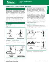
The flow of water in a conduit may be either open channel flow or pipe flow. The two kinds of 

flow are similar in many ways but differ in one important respect. Open-channel flow must have 

a free surface, whereas pipe flow has none. A free surface is subject to atmospheric pressure. In 

Pipe flow there exist no direct atmospheric flow but hydraulic pressure only. 

Energy line 

Hydraulic 

gradient 

Centre line 

1 2 

hf 

2 v /2g 

y 

z 

Energy line 

Water 

surface 

Channel bed 

Figure of pipe and open channel flow 

1 

2 

hf 

2 

v /2g 

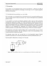
The two kinds of flow are compared in the figure above. On the left is pipe flow. Two 

piezometers are placed in the pipe at sections 1 and 2. The water levels in the pipes are 

maintained by the pressure in the pipe at elevations represented by the hydraulics grade line or 

hydraulic gradient. The pressure exerted by the water in each section of the pipe is shown in the 

tube by the height y of a column of water above the centre line of the pipe. 

The total energy of the flow of the section (with reference to a datum) is the sum of the elevation 

z of the pipe centre line, the piezometric head y and the velocity head V 2 /2g , where V is the 

mean velocity. The energy is represented in the figure by what is known as the energy grade line 

or the energy gradient. 

The loss of energy that results when water flows from section 1 to section 2 is represented by hf. 

A similar diagram for open channel flow is shown to the right. This is simplified by assuming 

parallel flow with a uniform velocity distribution and that the slope of the channel is small. In 

this case the hydraulic gradient is the water surface as the depth of water corresponds to the 

piezometric height. 

Despite the similarity between the two kinds of flow, it is much more difficult to solve problems 

of flow in open channels than in pipes. Flow conditions in open channels are complicated by the 

position of the free surface which will change with time and space. And also by the fact that 

depth of flow, the discharge, and the slopes of the channel bottom and of the free surface are all 

inter dependent. 

Physical conditions in open-channels vary much more than in pipes – the cross-section of pipes 

is usually round – but for open channel it can be any shape. 

Treatment of roughness also poses a greater problem in open channels than in pipes. Although 

there may be a great range of roughness in a pipe from polished metal to highly corroded iron, 


y 

z 

2

open channels may be of polished metal to natural channels with long grass and roughness that 

may also depend on depth of flow. 

Open channel flows are found in large and small scale. For example the flow depth can vary 

between a few cm in water treatment plants and over 10m in large rivers. The mean velocity of 

flow may range from less than 0.01 m/s in tranquil waters to above 50 m/s in high-head 

spillways. The range of total discharges may extend from 0.001 l/s in chemical plants to greater 

than 10000 m 3 /s in large rivers or spillways. 

In each case the flow situation is characterised by the fact that there is a free surface whose 

position is NOT known beforehand – it is determined by applying momentum and continuity 

principles. 

Open channel flow is driven by gravity rather than by pressure work as in pipes. 

Pipe flow Open Channel flow 

Flow driven by Pressure work Gravity (potential energy) 

Flow cross section Known, fixed Unknown in advance 

because the flow depth is 

Characteristics flow 

parameters 

Specific boundary 

conditions 

1.2 Types of flow 

velocity deduced from 

continuity 

unknown 

Flow depth deduced 

simultaneously from 

solving both continuity 

and momentum equations 

Atmospheric pressure at 

the free surface 

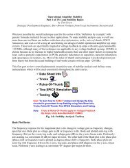
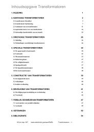
The following classifications are made according to change in flow depth with respect to time 

and space. 

RVF 

RVF GVF RVF GVF RVF GVF RVF GVF 

Figure of the types of flow that may occur in open channels 


3

Steady and Unsteady: Time is the criterion. 

Flow is said to be steady if the depth of flow at a particular point does not change or can be 

considered constant for the time interval under consideration. The flow is unsteady if depth 

changes with time. 

Uniform Flow: Space as the criterion. 

Open Channel flow is said to be uniform if the depth and velocity of flow are the same at every 

section of the channel. Hence it follows that uniform flow can only occur in prismatic channels. 

For steady uniform flow, depth and velocity is constant with both time and distance. This 

constitutes the fundamental type of flow in an open channel. It occurs when gravity forces are in 

equilibrium with resistance forces. 

Steady non-uniform flow. 

Depth varies with distance but not with time. This type of flow may be either (a) gradually 

varied or (b) rapidly varied. Type (a) requires the application of the energy and frictional 

resistance equations while type (b) requires the energy and momentum equations. 

Unsteady flow 

The depth varies with both time and space. This is the most common type of flow and requires 

the solution of the energy momentum and friction equations with time. In many practical cases 

the flow is sufficiently close to steady flow therefore it can be analysed as gradually varied 

steady flow. 

1.3 Properties of open channels 

Artificial channels 

These are channels made by man. They include irrigation canals, navigation canals, spillways, 

sewers, culverts and drainage ditches. They are usually constructed in a regular cross-section 

shape throughout – and are thus prismatic channels (they don’t widen or get narrower along the 

channel. In the field they are commonly constructed of concrete, steel or earth and have the 

surface roughness’ reasonably well defined (although this may change with age – particularly 

grass lined channels.) Analysis of flow in such well defined channels will give reasonably 

accurate results. 

Natural channels 

Natural channels can be very different. They are not regular nor prismatic and their materials of 

construction can vary widely (although they are mainly of earth this can possess many different 

properties.) The surface roughness will often change with time distance and even elevation. 

Consequently it becomes more difficult to accurately analyse and obtain satisfactory results for 

natural channels than is does for man made ones. The situation may be further complicated if the 

boundary is not fixed i.e. erosion and deposition of sediments. 

Geometric properties necessary for analysis 

For analysis various geometric properties of the channel cross-sections are required. For artificial 

channels these can usually be defined using simple algebraic equations given y the depth of flow. 

The commonly needed geometric properties are shown in the figure below 

and defined as: 


4

Depth (y) – the vertical distance from the lowest point of the channel section to the free surface. 

Stage (z) – the vertical distance from the free surface to an arbitrary datum 

Area (A) – the cross-sectional area of flow, normal to the direction of flow 

Wetted perimeter (P) – the length of the wetted surface measured normal to the direction of 

flow. 

Surface width (B) – width of the channel section at the free surface 

Hydraulic radius (R) – the ratio of area to wetted perimeter (A/P) 

Hydraulic mean depth (Dm) – the ratio of area to surface width (A/B) 

Rectangle Trapezoid Circle 

B 

B 

b 

y 

Area, A by (b+xy)y ( ) 2 

1 x 

b 

y 

D 

8 

φ 

1 φ − sinφ D 

Wetted perimeter P b + 2y 

b + 2y 2 

1+ 

x 

1 

2 φD 

Top width B b b+2xy ( sinφ 2)D 

Hydraulic radius R 

Hydraulic mean 

depth Dm 

by ( b + 2y 

) 

y 

( b + xy) 

y 

2 

b + 2y 1+ 

x 

( b + xy) 

y 

b + 2xy 

1 ⎛ sinφ 

⎞ 

⎜1− 

⎟D 

4 ⎝ φ ⎠ 

1 ⎛ φ − sinφ 

⎞ 

⎜ ⎟ 

8 ⎝ sin 1/ 

2φ 

⎠ 

( ) D 

Table of equations for rectangular trapezoidal and circular channels. 

1.4 Fundamental equations 

The equations which describe the flow of fluid are derived from three fundamental laws of 

physics: 

1. Conservation of matter (or mass) 

2. Conservation of energy 

3. Conservation of momentum 

Although first developed for solid bodies they are equally applicable to fluids. A brief 

description of the concepts are given below. 

Conservation of matter 

This says that matter can not be created nor destroyed, but it may be converted (e.g. by a 

chemical process.) In fluid mechanics we do not consider chemical activity so the law reduces to 

one of conservation of mass. 

Conservation of energy 

This says that energy can not be created nor destroyed, but may be converted form one type to 

another (e.g. potential may be converted to kinetic energy). When engineers talk about energy 

"losses" they are referring to energy converted from mechanical (potential or kinetic) to some 

other form such as heat. A friction loss, for example, is a conversion of mechanical energy to 

heat. The basic equations can be obtained from the First Law of Thermodynamics but a 

simplified derivation will be given below. 


d 

5

Conservation of momentum 

The law of conservation of momentum says that a moving body cannot gain or lose momentum 

unless acted upon by an external force. This is a statement of Newton's Second Law of Motion: 

Force = rate of change of momentum 

In solid mechanics these laws may be applied to an object which is has a fixed shape and is 

clearly defined. In fluid mechanics the object is not clearly defined and as it may change shape 

constantly. To get over this we use the idea of control volumes. These are imaginary volumes of 

fluid within the body of the fluid. To derive the basic equation the above conservation laws are 

applied by considering the forces applied to the edges of a control volume within the fluid. 

1.4.1 The Continuity Equation (conservation of mass) 

For any control volume during the small time interval δt the principle of conservation of mass 

implies that the mass of flow entering the control volume minus the mass of flow leaving the 

control volume equals the change of mass within the control volume. 

If the flow is steady and the fluid incompressible the mass entering is equal to the mass leaving, 

so there is no change of mass within the control volume. 

So for the time interval δt: 

A1 

V1 

A2 

V2 

Mass flow entering = mass flow leaving 

z1 

Figure of a small length of channel as a control volume 

y1 

d1 

θ 

z2 

y2 

surface 

Considering the control volume above which is a short length of open channel of arbitrary crosssection 

then, if ρ is the fluid density and Q is the volume flow rate then 

mass flow rate is ρQ and the continuity equation for steady incompressible flow can be written 

ρ Q = ρQ 

entering 

As, Q, the volume flow rate is the product of the area and the mean velocity then at the upstream 

leaving 

face (face 1) where the mean velocity is u1 and the cross-sectional area is A1 then: 

Q = u 

entering 1 1 

Similarly at the downstream face, face 2, where mean velocity is u2 and the cross-sectional area 

is A2 then: 


A 

bed 

6

Q = u 

leaving 

Therefore the continuity equation can be written as 

u A = u 

1.4.2 The Energy equation (conservation of energy) 

1 

1 

2 

2 

A 

A 

2 

2 

Equation 1.1 

Consider the forms of energy available for the above control volume. If the fluid moves from the 

upstream face 1, to the downstream face 2 in time δt over the length L. 

The work done in moving the fluid through face 1 during this time is 

where p1 is pressure at face 1 

The mass entering through face 1 is 

work done = 

Therefore the kinetic energy of the system is: 

p1 1 

mass entering = ρ 

1 

2 

1 

2 

2 

KE = mu = ρ1 

A L 

1A1 

1 

L 

A Lu 

If z1 is the height of the centroid of face 1, then the potential energy of the fluid entering the 

control volume is : 

PE = mgz = ρ A L g z 

The total energy entering the control volume is the sum of the work done, the potential and the 

kinetic energy: 

1 

2 

Total energy = p1 A1L 

+ ρ 1A1 

Lu1 

+ ρ1 

A1Lgz1 

2 

We can write this in terms of energy per unit weight. As the weight of water entering the control 

volume is ρ1 A1 L g then just divide by this to get the total energy per unit weight: 

2 

p1 

u1 

Total energy per unit weight 

= + + z1 

ρ g 2g 

At the exit to the control volume, face 2, similar considerations deduce 

2 

2 2 

Total energy per unit weight 

= + + z2 

ρ 2 g 2g 

If no energy is supplied to the control volume from between the inlet and the outlet then energy 

leaving = energy entering and if the fluid is incompressible ρ1 = ρ1 = ρ 


1 

1 

1 

p 

1 

2 

1 

u 

7

So, 

This is the Bernoulli equation. 

2 

2 

p1 

u1 

p2 

u2 

+ + z1 

= + + z2 

= H = constant 

ρg 

2g 

ρg 

2g 

Equation 1.2 

Note: 

1. In the derivation of the Bernoulli equation it was assumed that no energy is lost in the control 

volume - i.e. the fluid is frictionless. To apply to non frictionless situations some energy loss 

term must be included 

2. The dimensions of each term in equation 1.2 has the dimensions of length ( units of meters). 

For this reason each term is often regarded as a "head" and given the names 

p 

ρg 

= 

2 

u 

= 

2g 

pressure head 

velocity head 

z = velocity or potential head 

3. Although above we derived the Bernoulli equation between two sections it should strictly 

speaking be applied along a stream line as the velocity will differ from the top to the bottom 

of the section. However in engineering practise it is possible to apply the Bernoulli equation 

with out reference to the particular streamline 

1.4.3 The momentum equation (momentum principle) 

Again consider the control volume above during the time δt 

momentum entering 

momentum leaving 

= ρδQ 

δtu 

2 

1 

= ρδQ 

δtu 

By the continuity principle : δQ1 = δQ2 = δQ 

And by Newton's second law Force = rate of change of momentum 

δF 

= 

= 

momentum leaving - momentum entering 

δt 

ρδQ 

( u − u ) 

2 

1 

It is more convenient to write the force on a control volume in each of the three, x, y and z 

direction e.g. in the x-direction 

δ 

( u u ) 

Fx = ρδQ 

2x − 1x 


2 

1 

8

Integration over a volume gives the total force in the x-direction as 

( V V ) 

Fx = ρ Q 2x − 1x 

As long as velocity V is uniform over the whole cross-section. 

This is the momentum equation for steady flow for a region of uniform velocity. 

Energy and Momentum coefficients 

Equation 1.3 

In deriving the above momentum and energy (Bernoulli) equations it was noted that the velocity 

must be constant (equal to V) over the whole cross-section or constant along a stream-line. 

Clearly this will not occur in practice. Fortunately both these equation may still be used even for 

situations of quite non-uniform velocity distribution over a section. This is possible by the 

introduction of coefficients of energy and momentum, α and β respectively. 

These are defined: 

where V is the mean velocity. 

3 

ρu 

dA 

α 3 

ρV 

A 

∫ = 

2 

∫ ρu 

dA 

β = 2 

ρV 

A 

And the Bernoulli equation can be rewritten in terms of this mean velocity: 

And the momentum equation becomes: 

2 

p αV 

+ + z = constant 

ρg 

2g 

( V V ) 

Fx = ρ Qβ 

2x − 1x 

Equation 1.4 

Equation 1.5 

Equation 1.6 

Equation 1.7 

The values of α and β must be derived from the velocity distributions across a cross-section. 

They will always be greater than 1, but only by a small amount consequently they can often be 

confidently omitted – but not always and their existence should always be remembered. For 

turbulent flow in regular channel α does not usually go above 1.15 and β will normally be below 

1.05. We will see an example below where their inclusion is necessary to obtain accurate results. 

1.5 Velocity distribution in open channels 

The measured velocity in an open channel will always vary across the channel section because of 

friction along the boundary. Neither is this velocity distribution usually axisymmetric (as it is in 

pipe flow) due to the existence of the free surface. It might be expected to find the maximum 

velocity at the free surface where the shear force is zero but this is not the case. The maximum 


9

velocity is usually found just below the surface. The explanation for this is the presence of 

secondary currents which are circulating from the boundaries towards the section centre and 

resistance at the air/water interface. These have been found in both laboratory measurements and 

3d numerical simulation of turbulence. 

The figure below shows some typical velocity distributions across some channel cross sections. 

The number indicates percentage of maximum velocity. 

Figure of velocity distributions 

1.5.1 Determination of energy and momentum coefficients 

To determine the values of α and β the velocity distribution must have been measured (or be 

known in some way). In irregular channels where the flow may be divided into distinct regions α 

may exceed 2 and should be included in the Bernoulli equation. 

The figure below is a typical example of this situation. The channel may be of this shape when a 

river is in flood – this is known as a compound channel. 

Figure of a compound channel with three regions of flow 

If the channel is divided as shown into three regions and making the assumption that α = 1 for 

each then 


10

where 

1.6 Laminar and Turbulent flow 

3 

u dA 3 

V1 

A1 

+ V 

= = 3 

3 

V A V 

∫ α 

V 

1 

( A + A + A ) 

1 

3 

2 

2 

A + V 

2 

2 

3 

3 

3 

Q V1 

A1 

+ V2 

A2 

+ V3 

A3 

= = 

A A + A + A 

As in pipes , and all flow, the flow in an open channel may be either laminar or turbulent. The 

criterion for determining the type of flow is the Reynolds Number, Re. 

For pipe flow 

ρuD 

Re = 

µ 

And the limits for reach type of flow are 

Laminar: Re < 2000 

Turbulent: Re > 4000 

If we take the characteristic length as the hydraulic radius R = A/P then for a pipe flowing full R 

= D/4 and 

Re 

channel 

ρuR ρuD 

Re 

= = = 

µ µ 4 4 

So for an open channel the limits for each type of flow become 

3 

pipe 

Laminar: Re channel < 500 

Turbulent: Re channel > 1000 

In practice the limit for turbulent flow is not so well defined in channel as it is in pipes and so 

2000 is often taken as the threshold for turbulent flow. 

We can use the ideas seen for pipe flow analysis to look at the effect of friction. Taking the 

Darcy-Wiesbach formula for head loss due to friction in a pipe in turbulent flow 

h f 

4 fLV 

= 

2gD 

and make the substitution for hydraulic radius R = D/4 

And if we put the bed slope So = L/hf then 

and 

S o 

V 

2 

2 

4 fV 

= 

2g 

4R 

2gRS 

8gRSo 

o 

λ = f = 

2 

2 


V 

A 

3 

11

The Colebrook-White equation gives the f - Re relationship for pipes, putting in R=D/4 the 

equivalent equation for open channel is 

1 

f 

= −4log 

where ks is the effective roughness height 

10 

⎛ 

⎞ 

⎜ 

k s 1. 

26 

+ ⎟ 

⎜ 

⎟ 

⎝ 

14. 

8R 

Re f ⎠ 

A chart of the λ - Re relationship for open channels can be drawn using this equation but its 

practical application is not clear. In pipes this relationship is useful but due to the more complex 

flow pattern and the extra variable (R varies with depth and channel shape) then it is difficult to 

apply to a particular channel. 

In practice flow in open channels is usually in the rough turbulent zone and consequently simpler 

friction formulae may be applied to relate frictional losses to velocity and channel shape. 

1.7 Uniform flow and the Development of Friction formulae 

When uniform flow occurs gravitational forces exactly balance the frictional resistance forces 

which apply as a shear force along the boundary (channel bed and walls). 

V 

τ 

θ 

L 

weight 

surface 

bed 

Figure of forces on a channel length in uniform flow 

Considering the above diagram, the gravity force resolved in the direction of flow is 

gravity force = ρgAL sinθ 

and the boundary shear force resolved in the direction of flow is 

In uniform flow these balance 

shear force = τ o PL 

τ PL ρgALsinθ 

o = 

Considering a channel of small slope, (as channel slopes for unifor and gradually varied flow 

seldom exceed about 1 in 50) then 

sin θ ≈ tanθ 

= So 

So 


12

1.7.1 The Chezy equation 

ρgAS 

P 

o τ o = = 

ρgRS 

If an estimate of τo can be made then we can make use of Equation 1.8. 

o 

Equation 1.8 

If we assume the state of rough turbulent flow then we can also make the assumption the shear 

force is proportional to the flow velocity squared i.e. 

Substituting this into equation 1.8 gives 

V 

τ ∝ V 

o 

2 

τ = KV 

= 

o 

ρg 

K 

Or grouping the constants together as one equal to C 

V = C 

This is the Chezy equation and the C the “Chezy C” 

Because the K is not constant the C is not constant but depends on Reynolds number and 

boundary roughness (see discussion in previous section). 

2 

RSo 

RSo 

Equation 1.9 

The relationship between C and λ is easily seen be substituting equation 1.9 into the Darcy- 

Wiesbach equation written for open channels and is 

1.7.2 The Manning equation 

C = 

A very many studies have been made of the evaluation of C for different natural and manmade 

channels. These have resulted in today most practising engineers use some form of this 

relationship to give C: 

2g 

f 

1 

R 

C = 

n 

This is known as Manning’s formula, and the n as Manning’s n. 

/ 6 

Equation 1.10 


13

Substituting equation 1.9 in to 1.10 gives velocity of uniform flow: 

Or in terms of discharge 

2/ 

3 1 

R So 

V = 

n 

1 A 

Q = 

n P 

5/ 

3 

2/ 

3 

/ 2 

S 

1/ 

2 

o 

Equation 1.11 

Note: 

Several other names have been associated with the derivation of this formula – or ones similar 

and consequently in some countries the same equation is named after one of these people. Some 

of these names are; Strickler, Gauckler, Kutter, Gauguillet and Hagen. 

The Manning’s n is also numerically identical to the Kutter n. 

The Manning equation has the great benefits that it is simple, accurate and now due to it long 

extensive practical use, there exists a wealth of publicly available values of n for a very wide 

range of channels. 

Below is a table of a few typical values of Manning’s n 

Channel type Surface material and form Manning’s n range 

River earth, straight 0.02-0.025 

earth, meandering 0.03-0.05 

gravel (75-150mm), straight 0.03-0.04 

gravel (75-150mm), winding 0.04-0.08 

unlined canal earth, straight 0.018-0.025 

rock, straight 0.025-0.045 

lined canal concrete 0.012-0.017 

lab. models mortar 0.011-0.013 

Perspex 0.009 

1.7.3 Conveyance 

Channel conveyance, K, is a measure of the carrying capacity of a channel. The K is really an 

agglomeration of several terms in the Chezy or Manning's equation: 

Q = AC RS 

So 

Q = KS 

1/ 

2 

o 

1/ 

2 

K = ACR = 

o 

A 

nP 

5 / 3 

2 / 3 

Equation 1.12 

Equation 1.13 

Use of conveyance may be made when calculating discharge and stage in compound channels 

and also calculating the energy and momentum coefficients in this situation. 


14

1.8 Computations in uniform flow 

We can use Manning's formula for discharge to calculate steady uniform flow. Two calculations 

are usually performed to solve uniform flow problems. 

1. Discharge from a given depth 

2. Depth for a given discharge 

In steady uniform flow the flow depth is know as normal depth. 

As we have already mentioned, and by definition, uniform flow can only occur in channels of 

constant cross-section (prismatic channels) so natural channel can be excluded. However we will 

need to use Manning's equation for gradually varied flow in natural channels - so application to 

natural/irregular channels will often be required. 

1.8.1 Uniform flow example 1 - Discharge from depth in a trapezoidal channel 

A concrete lined trapezoidal channel with uniform flow has a normal depth is 2m. 

The base width is 5m and the side slopes are equal at 1:2 

Manning's n can be taken as 0.015 

And the bed slope S0 = 0.001 

What are: 

a) Discharge (Q) 

b) Mean velocity (V) 

c) Reynolds number (Re) 

Calculate the section properties 

A = 

Use equation 1.11 to get the discharge 

( 5 + 2y 

) 

P = 5 + 2y 

5 / 3 

1 A 

= S 2 / 3 

n P 

3 

= 45m 

/ s 

1/ 

2 

Q o 

= 

y = 18m 

1+ 

2 

2 

1 

0. 

015 

2 

= 13. 

94m 

5 

18 

13. 

94 

/ 3 

2 / 3 

0. 

001 

The simplest way to calculate the mean velocity is to use the continuity equation: 

Q 45 

V = = = 2. 

5m 

/ s 

A 18 

And the Reynolds number (R=A/P) 

3 

ρuR 

ρuA 

10 × 2. 

5× 

18 

6 

Re channel = = = 

= 2. 

83× 

10 

−3 

µ µ P 1. 

14× 

10 × 13. 

94 

This is very large - i.e. well into the turbulent zone - the application of the Manning's equation 

was therefore valid. 


1/ 

2 

15

What solution would we have obtained if we had used the Colebrook-White equation? 

Probably very similar as we are well into the rough-turbulent zone where both equations are truly 

applicable. 

To experiment an equivalent ks value can be calculated for the discharge calculated from n = 

0.015 and y = 2m [ks = 2.225mm] (Use the Colebrook-White equation and the Darcy-Wiesbach 

equation of open channels - both given earlier). Then a range of depths can be chosen and the 

discharges calculated for these n and ks values. Comparing these discharge calculations will give 

some idea of the relative differences - they will be very similar. 

1.8.2 Uniform flow example 2 - Depth from Discharge in a trapezoidal channel 

Using the same channel as above, if the discharge is know to be 30m 3 /s in uniform flow, what is 

the normal depth? 

Again use equation 1.11 

2 

A = 5 + 2y 

y = 18m 

( ) 

P = 5 + 2y 

1+ 

2 

2 

= 13. 

94m 

Q = 

30 = 

1 

0. 

015 

2. 

108 

We need to calculate y from this equation. 

( ( 5 + 2y 

) y) 

2 

( 5 + 2y 

1+ 

2 ) 

( ( 5 + 2y 

) y) 

5 / 3 

5 / 3 

2 / 3 

( ) 3 / 2 

2 

5 + 2y 

1+ 

2 

0. 

001 

Even for this quite simple geometry the equation we need to solve for normal depth is complex. 

One simple strategy to solve this is to select some appropriate values of y and calculate the right 

hand side of this equation and compare it to Q (=30) in the left. When it equals Q we have the 

correct y. Even though there will be several solutions to this equation, this strategy generally 

works because we have a good idea of what the depth should be (e.g. it will always be positive 

and often in the range of 0.5-10 m). 

In this case from the previous example we know that at Q = 45 m 3 /s, y = 2m. So at Q = 30 m 3 /s 

then y < 2.0m. 

Guessed y (m) Discharge Q (m 3 /s) 

1.7 32.7 

1.6 29.1 

1.63 30.1 

You might also use the bisector method to solve this. 


1/ 

2 

16

1.8.3 Uniform flow example 3 - A compound channel 

If the channel in the above example were to be designed for flooding it may have a section like 

this: 

1 

3 

14.5 

10 

1 

2 

15.0 

5 

Figure of compound section 

10 

14.5 

region 2 region 1 region 3 

4 

When the flow goes over the top of the trapezoidal channel it moves to the "flood plains" so the 

section allows for a lot more discharge to be carried. 

If the flood channels are 10m wide and have side slopes of 1:3, and the Manning n on these 

banks is0.035, what are 

a) the discharge for a flood level of 4m 

b) the enery coefficient α 

First split the section as shown in to three regions (this is arbitrary - left to the engineers 

judgement). Then apply Manning's formula for each section to give three discharge values and 

the total discharge will be Q = Q1 + Q2 + Q3. 

Calculate the properties of each region: 

⎛ 5 + 15 ⎞ 

A 1 = ⎜ ⎟2. 

5 + = 

⎝ 2 ⎠ 

⎛ 10 + 14. 

5 ⎞ 

A 2 = A3 

= ⎜ ⎟1. 

5 = 18. 

38m 

⎝ 2 ⎠ 

2 

( 15× 

1. 

5) 

47. 

5m 

( 2 5 × 2. 

5) 

= 16. 

m 

+ ( 1. 

5 10) 

= 14. 

m 

P = 5 + 

18 

1 

P = P = 10 

75 

2 

The conveyance for each region may be calculated from equation 1.13 

K 

K 

2 

1 

3 

5 / 3 

47. 

5 

= 

0. 

015× 

16. 

18 

= K 

3 

2 / 3 

5 / 3 

18. 

38 

= 

0. 

035× 

14. 

74 

= 

2 / 3 

6492. 

5 

= 

2 

608. 

4 


17

And from Equation 1.11 or Equation 1.12 the discharges 

or 

And 

or 

So 

Q 

Q 

1 

1 

= 

0. 

015 

47. 

5 

16. 

18 

5 / 3 

2 / 3 

0. 

001 

1/ 

2 

1/ 

2 

3 

Q = K 0. 

001 = 205. 

3m 

/ s 

2 

1 

= Q 

3 

1 

1 

= 

0. 

035 

18. 

38 

14. 

74 

5 / 3 

2 / 3 

0. 

001 

1/ 

2 

1/ 

2 

2 

Q = Q = K 0. 

001 = 19. 

2m 

/ s 

2 

3 

2 

3 

Q = Q + Q + Q = 243. 

7m 

/ s 

The velocities can be obtained from the continuity equation: 

Q1 

V1 

= = 4. 

32m 

/ s 

A 

Q2 

V2 

= V3 

= = 1. 

04m 

/ s 

A2 

And the energy coefficient may be obtained from Equation 1.4 

where 

Giving 

1 

3 

u dA 3 

V1 

A1 

+ V 

= = 3 

3 

V A V 

∫ α 

V 

1 

2 

1 

3 

( A + A + A ) 

1 

3 

2 

2 

A + V 

2 

2 

3 

3 

3 

Q V1 

A1 

+ V2 

A2 

+ V3 

A3 

= = 

A A + A + A 

α = 1. 

9 

This is a very high value of α and a clear case of where a velocity coefficient should be used. 

Not that this method doe not give completely accurate relationship between stage and discharge 

because some of the assumptions are not accurate. E.g. the arbitrarily splitting in to regions of 

fixed Manning n is probably not what is occurring in the actual channel. However it will give an 

acceptable estimate as long as care is taken in choosing these regions. 

1.9 The Application of the Energy equation for Rapidly Varied Flow 

Rapid changes in stage and velocity occur whenever there is a sudden change in cross-section, a 

very steep bed-slope or some obstruction in the channel. This type of flow is termed rapidly 

varied flow. Typical example are flow over sharp-crested weirs and flow through regions of 

greatly changing cross-section (Venturi flumes and broad-crested weirs). 

Rapid change can also occur when there is a change from super-critical to sub-critical flow (see 

later) in a channel reach at a hydraulic jump. 


3 

A 

3 

18

In these regions the surface is highly curved and the assumptions of hydro static pressure 

distribution and parallel streamlines do not apply. However it is possibly to get good 

approximate solutions to these situations yet still use the energy and momentum concepts 

outlined earlier. The solutions will usually be sufficiently accurate for engineering purposes. 

1.9.1 The energy (Bernoulli) equation 

The figure below shows a length of channel inclined at a slope of θ and flowing with uniform 

flow. 

Figure of channel in uniform flow 

Recalling the Bernoulli equation (1.6) 

2 

p αV 

+ + z = constant 

ρg 

2g 

And assuming a hydrostatic pressure distribution we can write the pressure at a point on a 

streamline, A say, in terms of the depth d (the depth measured from the water surface in a 

direction normal to the bed) and the channel slope. 

p A 

= ρgd 

[Note: in previous derivation we used y in stead of d – they are the same.] 

In terms of the vertical distance 

So 

y2 

d = = y1 

cosθ 

cosθ 

2 

y = y cos θ 

2 

1 

pA = ρgy 

2 

1 cos 


θ 

19

So the pressure term in the above Bernoulli equation becomes 

pA 2 

= y1 

cos 

ρg 

As channel slope in open channel are very small (1:100 ≡ θ = 0.57 and 

cos 2 θ = 0.9999) so unless the channel is unusually steep 

pA = y1 

ρg 

And the Bernoulli equation becomes 

θ 

2 

V 

y + + z = H 

2g 

α 

1.9.2 Flow over a raised hump - Application of the Bernoulli equation 

Equation 1.14 

Steady uniform flow is interrupted by a raised bed level as shown. If the upstream depth and 

discharge are known we can use equation 1.14 and the continuity equation to give the velocity 

and depth of flow over the raised hump. 

Figure of the uniform flow interrupted by a raised hump 

Apply the Bernoulli equation between sections 1 and 2. (assume a horizontal rectangular channel 

z1 = z2 and take α = 1) 

2 

2 

V1 

V2 

y1 + = y2 

+ + ∆z 

2g 

2g 

Equation 1.15 

use the continuity equation 


20

Where q is the flow per unit width. 

V A = V A = Q 

1 

V y = V y 

1 

1 

1 

2 

2 

2 

2 

Q 

= = q 

B 

Substitute this into the Bernoulli equation to give: 

2 

2 

q q 

y1 + = y + + ∆z 

2 2 2 

2gy 

2gy 

rearranging: 

2gy 

3 

2 

1 

2 

⎛ 

q ⎞ 

2 

+ y ⎜ 

2 2g∆z 

− 2gy 

⎟ 

1 − + q 

⎜ 

2 ⎟ 

⎝ 

y1 

⎠ 

Thus we have a cubic with the only unknown being the downstream depth, y2. There are three 

solutions to this - only one is correct for this situation. We must find out more about the flow 

before we can decide which it is. 

1.9.3 Specific Energy 

The extra information needed to solve the above problem can be provided by the specific energy 

equation. 

Specific energy, Es, is defined as the energy of the flow with reference to the channel bed as the 

datum: 

E s 

αV 

= y + 

2g 

For steady flow this can be written in terms of discharge Q 

E s 

α 

= y + 

For a rectangular channel of width b, Q/A = q/y 

( E − y) 

s 

E 

y 

s 

2 

2 

2 

( Q / A) 

2g 

2 

αq 

= y + 

2gy 

2 

αq 

= = constant 

2g 

2 

2 

2 

= 0 

Equation 1.16 

constant 

( Es 

− y) 

= 2 

y 

This is a cubic in y. It has three solutions but only two will be positive (so discard the other). 


21

1.9.4 Flow over a raised hump - revisited. Application of the Specific energy equation. 

The specific energy equation may be used to solve the raised hump problem. The figure below 

shows the hump and stage drawn alongside a graph of Specific energy Es against y. 

Figure of raised bed hump and graph of specific energy 

The Bernoulli equation was applied earlier to this problem and equation (from that example) 

1.15 may be written in terms of specify energy: 

= 2 

Es1 Es 

+ ∆z 

These points are marked on the figure. Point A on the curve corresponds to the specific energy at 

point 1 in the channel, but Point B or Point B' on the graph may correspond to the specific 

energy at point 2 in the channel. 

All point in the channel between point 1 and 2 must lie on the specific energy curve between 

point A and B or B'. To reach point B' then this implies that ES1 - ES2 > ∆z which is not 

physically possible. So point B on the curve corresponds to the specific energy and the flow 

depth at section 2. 

1.9.5 Example of the raised bed hump. 

A rectangular channel with a flat bed and width 5m and maximum depth 2m has a discharge of 

10m 3 /s. The normal depth is 1.25 m. What is the depth of flow in a section in which the bed rises 

0.2m over a distance 1m. 

Assume frictional losses are negligible. 

= 2 

Es1 Es 

+ ∆z 


22

Es 2 

Es 1 

= y 

⎛ 10 ⎞ 

⎜ ⎟ 

1. 

25 5 

1. 

25 

⎝ × 

= + 

⎠ 

2g 

2 

1. 

38 

1. 

18 

⎛ 10 ⎞ 

⎜ 

5 y ⎟ 

⎝ × 2 

+ 

⎠ 

2g 

= y 

2 

= y 

2 

2 

= y 

2 

2 

2 

2 

2 

2 

0. 

2039 

+ + 

y 

0. 

2039 

+ = 

y 

Again this can be solved by a trial and error method: 

y2 

Es2 

0.9 1.15 

1.0 1.2 

0.96 1.18 

= 1. 

38 

0. 

2039 

+ 

y 

i.e. the depth of the raised section is 0.96m or the water level (stage) is 1.16m a drop of 9cm 

when the bed has raised 20cm. 

1.10 Critical , Sub-critical and super critical flow 

The specific energy change with depth was plotted above for a constant discharge Q, it is also 

possible to plot a graph with the specific energy fixed and see how Q changes with depth. These 

two forms are plotted side by side below. 

0. 

2 

Figure of variation of Specific Energy and Discharge with depth. 

From these graphs we can identify several important features of rapidly varied flow. 

For a fixed discharge: 

1. The specific energy is a minimum, Esc, at depth yc, 

This depth is known as critical depth. 

2. For all other values of Es there are two possible depths. These are called alternate depths. For 

subcritical flow y > yc 

supercritical flow y < yc 


Es 

2 

2 

2 

23

For a fixed Specific energy 

1. The discharge is a maximum at critical depth, yc. 

2. For all other discharges there are two possible depths of flow for a particular Es 

i.e. There is a sub-critical depth and a super-critical depth with the same Es. 

An equation for critical depth can be obtained by setting the differential of Es to zero: 

E 

s 

α 

= y + 

( Q / A) 

2g 

2 

dEs 

αQ 

= 0 = 1+ 

dy 2g 

Since δ A = Bδy 

, in the limit dA/dy = B and 

αQ 

B 

gA 

2 

c 

3 

c 

= 1 

2 

αQ 

0 = 1− 

2g 

d 

dA 

2 

⎛ 1 

⎜ 

⎝ A 

c 

2 

B 2A 

⎞ dA 

⎟ 

⎠ dy 

−3 

c 

Equation 1.17 

For a rectangular channel Q = qb, B = b and A = by, and taking α = 1 this equation becomes 

as Vc yc= q 

y c 

c 

2 ⎛ q ⎞ 

= ⎜ 

⎟ 

⎝ g ⎠ 

V = 

Substituting this in to the specific energy equation 

2 

Vc 

Esc 

= yc 

+ = y 

2g 

y 

c 

= 

2 

3 

E 

sc 

gy 

1/ 

3 

c 

c 

yc 

+ 

2 

Equation 1.18 

Equation 1.19 


24

1.11 The Froude number 

The Froude number is defined for channels as: 

Fr = 

Equation 1.20 

Its physical significance is the ratio of inertial forces to gravitational forces squared 

2 

Fr = 

V 

gDm 

inertial force 

gravitational 

force 

It can also be interpreted as the ratio of water velocity to wave velocity 

water velocity 

Fr = 

wave velocity 

This is an extremely useful non-dimensional number in open-channel hydraulics. 

Its value determines the regime of flow – sub, super or critical, and the direction in which 

disturbances travel 

Fr < 1 sub-critical 

water velocity > wave velocity 

upstream levels affected by downstream controls 

Fr = 1 critical 

Fr > 1 super-critical 

water velocity < wave velocity 

upstream levels not affected by downstream controls 

Figure of sub and super critical flow and transmission of disturbances 


25

1.12 Application of the Momentum equation for Rapidly Varied Flow 

The hydraulic jump is an important feature in open channel flow and is an example of rapidly 

varied flow. A hydraulic jump occurs when a super-critical flow and a sub-critical flow meet. 

The jump is the mechanism for the to surface to join. They join in an extremely turbulent manner 

which causes large energy losses. 

Because of the large energy losses the energy or specific energy equation cannot be use in 

analysis, the momentum equation is used instead. 

Figure of forces applied to the control volume containing the hydraulic jump 

Or for a constant discharge 

Resultant force in x- direction = F1 - F2 

Momentum change = M2 – M1 

1 

F 

1 

F − F = M − M 

1 

+ M = F + M 

1 

1 

Q 

= ρQ 

y b 

1 

2 

2 

2 

2 

1 

= constant 

For a rectangular channel this may be evaluated using 

y1 

F1 

= ρg 

y1b 

2 

y2 

F2 

= ρg 

y2b 

2 

M = ρQV 

M = ρQV 

Substituting for these and rearranging gives 

Or 

y 

y 

2 

1 

2 ( 1+ 

8 1 −1) 

y1 

= Fr 

2 

2 ( 1+ 

8 2 −1) 

y2 

= Fr 

2 

2 

2 

Q 

= ρQ 

y b 

2 

Equation 1.21 

Equation 1.22 


26

So knowing the discharge and either one of the depths on the upstream or downstream side of the 

jump the other – or conjugate depth – may be easily computed. 

More manipulation with Equation 1.19 and the specific energy give the energy loss in the jump 

as 

3 ( y2 

− y1 

) 

∆ E = 

4y1 y2 

Equation 1.23 

These are useful results and which can be used in gradually varied flow calculations to determine 

water surface profiles. 

In summary, a hydraulic jump will only occur if the upstream flow is super-critical. The higher 

the upstream Froude number the higher the jump and the greater the loss of energy in the jump. 

1.13 Gradually varied flow 

In the previous section of rapidly varied flow little mention was made of losses due to friction or 

the influence of the bed slope. It was assumed that frictional losses were insignificant – this is 

reasonable because rapidly varied flow occurs over a very short distance. However when it 

comes to long distances they become very important, and as gradually varied flow occurs over 

long distances we will consider friction losses here. 

In the section on specific energy it was noted that there are two depth possible in steady flow for 

a given discharge at any point in the channel. (One is super-critical the other depth sub-critical.) 

The solution of the Manning equation results in only one depth – the normal depth. 

It is the inclusion of the channel slope and friction that allow us to decide which of the two 

depths is correct. i.e. the channel slope and friction determine whether the uniform flow in the 

channel is sub or super-critical. 

The procedure is 

i. Calculate the normal depth from Manning’s equation (1.11) 

ii. Calculate the critical depth from equation 1.17 

The normal depth may be greater, less than or equal to the critical depth. 

For a given channel and roughness there is only one slope that will give the normal depth equal 

to the critical depth. This slope is known as the critical slope (Sc). 

If the slope is less than Sc the normal depth will be greater than critical depth and the flow will 

be sub-critical flow. The slope is termed mild. 

If the slope is greater than Sc the normal depth will be less than critical depth and the flow will 

be super-critical flow. The slope is termed steep. 


27

1.13.1 Example of critical slope calculation 

We have Equation 1.11 that gives normal depth 

and equation 1.17 that given critical depth 

1 A 

Q = 

n P 

2 

αQ 

B 

3 

2gA 

Rearranging these in terms of Q and equating gives 

1 A 

n P 

5/ 

3 

2/ 

3 

S 

c 

5/ 

3 

2/ 

3 

c 

1/ 

2 

c 

For the simple case of a wide rectangular channel, width B = b, A = by and P≅b. And the above 

equation becomes 

2 

gn 

S c = 1/ 

3 

yc 

Equation 1.24 

S 

= 1 

= 

1/ 

2 

o 

1.13.2 Transitions between sub and super critical flow 

If sub critical flow exists in a channel of a mild slope and this channel meets with a steep channel 

in which the normal depth is super-critical there must be some change of surface level between 

the two. In this situation the surface changes gradually between the two. The flow in the joining 

region is known as gradually varied flow. 

This situation can be clearly seen in the figure on the left below. Note how at the point of joining 

of the two channels the depth passes through the critical depth. 

gA 

Figure of transition from sup to super-critical flow 


B 

3 

28

If the situation is reversed and the upstream slope is steep, super critical flow, and the down 

stream mild, sub-critical, then there must occur a hydraulic jump to join the two. There may 

occur a short length of gradually varied flow between the channel junction and the jump. The 

figure above right shows this situation: 

Analysis of gradually varied flow can identify the type of profile for the transition as well as the 

position hydraulic jumps. 

1.14 The equations of gradually varied flow 

The basic assumption in the derivation of this equation is that the change in energy with distance 

is equal to the friction loses. 

The Bernoulli equation is: 

dH 

= −S 

dx 

Differentiating and equating to the friction slope 

Or 

where So is the bed slope 

d 

dx 

2 

V 

y + + z = H 

2g 

α 

⎛ αV 

⎜ y + 

⎜ 

⎝ 2g 

dE 

dx 

2 

f 

⎞ 

⎟ = − 

⎟ 

⎠ 

dz 

dx 

s = So 

− S f 

We saw earlier how specific energy change with depth (derivation of Equation 1.17) 

dE 

dy 

Combining this with equation 1.25 gives 

s = + 

2 

c = 1+ 

3 

gAc 

− 

S f 

Q B 

1 Fr 

S 

− S 

dy o f 

= 2 

dx 

1− Fr 

2 

Equation 1.25 

Equation 1.26 

This is the basic equation of gradually varied flow. It describes how the depth, y, changes with 

distance x, in terms of the bed slope So, friction Sf and the discharge, Q, and channels shape 

(encompassed in Fr and Sf). 

Equations 1.25 and 1.26 are differential equations equating relating depth to distance. There is no 

explicit solution (except for a few special cases in prismatic channels). Numerical integration is 

the only practical method of solution. This is normally done on computers, however it is not too 

cumbersome to be done by hand. 


29

1.15 Classification of profiles 

Before attempting to solve the gradually varied flow equation a great deal of insight into the type 

of solutions and profiles possible can be gained by taking some time to examine the equation. 

Time spent over this is almost compulsory if you are to understand steady flow in open channels. 

For a given discharge, Sf and Fr 2 are functions of depth. 

S f 

Fr 

2 

2 2 

n Q P 

= 

A 

2 

Q B 

= 3 

gA 

A quick examination of these two expressions shows that they both increase with A, i.e. increase 

with y. 

10/ 

3 

We also know that when we have uniform flow 

S f = So 

and y = yn 

So 

and 

Sf > So when y < yn 

Sf < So when y > yn 

Fr 2 > 1 when y < yc 

Fr 2 < 1 when y > yc 

From these inequalities we can see how the sign of dy/dx i.e. the surface slope changes for 

different slopes and Froude numbers. 

Taking the example of a mild slope, shown in the figure below: 

4/ 

3 

Figure of zones / regions 

The normal and critical depths are shown (as it is mild normal depth is greater than critical 

depth). Treating the flow as to be in three zones: 


30

i. zone 1, above the normal depth 

ii. zone 2, between normal and critical depth 

iii. zone 3, below critical depth 

The direction of the surface inclination may thus be determined. 

zone 1 

y > yn > yc Sf < So Fr 2 < 1 dy/dx is positive, 

surface rising 

zone 2 

yn > y > yc Sf > So Fr 2 < 1 dy/dx is negative 

surface falling 

zone 3 

yn > yc > y Sf > So Fr 2 > 1 dy/dx is positive 

surface rising 

The condition at the boundary of the gradually varied flow may also be determined in a similar 

manner: 

zone 1 

As y → ∞ then Sf and Fr → 0 and dy/dx → So 

Hence the water surface is asymptotic to a horizontal line for it maximum 

As y → yn then Sf → So and dy/dx → 0 

Hence the water surface is asymptotic to the line y = yn i.e. uniform flow. 

zone 2 

As for zone 1 as y approached the normal depth: 

As y → yn then Sf → So and dy/dx → 0 

Hence the water surface is asymptotic to the line y = yn 

But a problem occurs when y approaches the critical depth: 

As y → yc then Fr → 1 and dy/dx → ∞ 

This is physically impossible but may be explained by the pointing out that in this region the 

gradually varied flow equation is not applicable because at this point the fluid is in the rapidly 

varied flow regime. 

In reality a very steep surface will occur. 

zone 3 

As for zone 2 a problem occurs when y approaches the critical depth: 

As y → yc then Fr → 1 and dy/dx → ∞ 


31

Again we have the same physical impossibility with the same explanation. 

And again in reality a very steep surface will occur. 

As y → 0 then dy/dx → So the slope of bed of the channel! 

The gradually varied flow equation is not valid here but it is clear what occurs. 

In general, normal depth is approached asymptotically and critical depth at right angles to the 

channel bed. 

The possible surface profiles within each zone can be drawn from the above considerations. 

These are shown for the mild sloped channel below. 

Figure of gradually varied flow surface profiles in a mild sloped channel 

The surface profile in zone 1 of a mild slope is called an M1 curve, in zone 2 an M2 curve and in 

zone 3 an M3 curve. 

All the possible surface profiles for all possible slopes of channel (there are 15 possibilities) are 

shown in the figure on the next page. 


32

Figure of the possible gradually varied flow profiles 


33

1.16 How to determine the surface profiles 

Before one of the profiles discussed above can be decided upon two things must be determined 

for the channel and flow: 

a) Whether the slope is mild, critical or steep. The normal and critical depths must be calculated 

for the design discharge 

b) The positions of any control points must be established. Control points are points of known 

depth or relationship between depth and discharge. Example are weirs, flumes, gates or 

points where it is known critical flow occurs like at free outfalls, or that the flow is normal 

depth at some far distance down stream. 

Once these control points and depth position has been established the surface profiles can be 

drawn to join the control points with the insertion of hydraulic jumps where it is necessary to 

join sub and super critical flows that don’t meet at a critical depth. 

Below are two examples. 

Figure of example surface profile due to a broad crested weir 

This shows the control point just upstream of a broad crested weir in a channel of mild slope. 

The resulting curve is an M1. 

Figure of example surface profile through a bridge when in floo 

This shows how a bridge may act as a control – particularly under flood conditions. Upstream 

there is an M1 curve then flow through the bridge is rapidly varied and the depth drops below 

critical depth so on exit is super critical so a short M3 curve occurs before a hydraulic jump takes 

the depth back to a sub-critical level. 


34

1.17 Method of solution of the Gradually varied flow equation 

There are three forms of the gradually varied flow equation: 

dH 

= −S 

f 

dx 

dE 

dx 

s = So 

− S f 

S 

− S 

dy o f 

= 2 

dx 

1− Fr 

Equation 1.26 

Equation 1.27 

Equation 1.28 

In the past direct and graphical solution methods have been used to solve these, however these 

method have been superseded by numerical methods which are now be the only method used. 

1.17.1 Numerical methods 

All (15) of the gradually varied flow profiles shown above may be quickly solved by simple 

numerical techniques. One computer program can be written to solve most situations. 

There are two basic numerical methods that can be used 

i. Direct step – distance from depth 

ii. Standard step method – depth from distance 

1.17.2 The direct step method – distance from depth 

This method will calculate (by integrating the gradually varied flow equation) a distance for a 

given change in surface height. 

The equation used is 1.28, which written in finite difference form is 

⎛ 

⎜ 

1− 

Fr 

∆x 

= ∆y 

⎜ 

⎝ So 

− S 

The steps in solution are: 

1. Determine the control depth as the starting point 

2. Decide on the expected curve and depth change if possible 

3. Choose a suitable depth step ∆y 

4. Calculate the term in brackets at the “mean” depth (yinitial + ∆y/2) 

5. Calculate ∆x 

6. Repeat 4 and 5 until the appropriate distance / depth changed reached 

2 

f 

⎞ 

⎟ 

⎠ 

mean 

Equation 1.29 

This is really best seen demonstrated in an example. [See the example on the web site for this 

module: www.efm.leeds.ac.uk/CIVE/CIVE2400] 


35

1.17.3 The standard step method – depth from distance 

This method will calculate (by integrating the gradually varied flow equation) a depth at a given 

distance up or downstream. 

The equation used is 1.27, which written in finite difference form is 

∆ E = ∆x 

− 

s 

( So 

S f ) mean 

Equation 1.30 

The steps in solution are similar to the direct step method shown above but for each ∆x there is 

the following iterative step: 

1. Assume a value of depth y (the control depth or the last solution depth) 

2. Calculate the specific energy EsG 

3. Calculate Sf 

4. Calculate ∆Es using equation 1.30 

5. Calculate ∆Es (x+∆x) = Es + ∆E 

6. Repeat until ∆Es (x+∆x) = EsG 

Again this is really best understood by means of an example. [See the example on the web site 

for this module: www.efm.leeds.ac.uk/CIVE/CIVE2400] 

1.17.4 The Standard step method – alternative form 

This method will again calculate a depth at a given distance up or downstream but this time the 

equation used is 1.26, which written in finite difference form is 

∆ H = −∆x 

( S f ) mean 

Equation 1.31 

Where H is given by equation 1.14 

2 

V 

y + + z = H 

2g 

α 

The strategy is the same as the first standard step method, with the same necessity to iterate for 

each step. 

1.18 Structures 

1.19 Critical depth meters 

The effect of a local rise in the bed level on the flow has been discussed earlier. It was shown 

that the depth would fall as the flow went over the rise. If this rise were large enough (for the 

particular velocity) the fall would be enough to give critical depth over the rise. Increasing the 

rise further would not decrease the depth but it would remain at critical depth. This observation 

may be confirmed by studying further the specific energy equation in a similar way to earlier. 


36

The fact that depth is critical over the rise and that critical depth can be calculated quite easily 

for a give discharge is made use of in hydraulic structures for flow measurement. Actually it is 

the converse of the above, that the discharge can be easily calculated if the critical depth is know, 

that is most useful. 

1.19.1 Broad-crested weir 

Figure of flow over a broad crested weir 

Assuming that the depth is critical over the rise then we know 

V = V = gy 

where b is the width of the channel 

Earlier Equation 1.19 it was shown that 

Assuming no energy loss between 1 and 2 

So 

2 

c 

Q = AV 

E 

s2 

y 

c 

c 

c 

= by 

c 

2 

y c = Es 

3 

H 

2 

gy 

2 

V1 

= h + = H 

2g 

= 

Q = 

2 

3 

2 

3 

2g 

bh 

3 

Q = 1. 

705bh 

in practice there are energy losses upstream of the weir. To incorporate this a coefficient of 

discharge and of velocity are introduced to give 

Q = CdCv 

3/ 

2 

3/ 

2 

1. 705bh 


c 

3/ 

2 

37

1.19.2 Flumes 

A second method of measuring flow by causing critical depth is to contract the flow. Similar 

specific energy arguments to those used for a raised bed can be used in analysis of this situation, 

and they come to similar predictions that depth will fall and not fall below critical depth. 

It is also possible to combine the two by putting a raised section within the narrowed section. 

These types of structures are known as flume, and the first type is known as a Venturi flume. 

1.19.3 Venturi flume 

Flumes are usually designed to achieve critical depth in the narrowest section (the throat) while 

also giving a very small afflux. 

Figure of section through a Venturi flume 

The general equation for the ideal discharge through a flume can be obtained from the energy 

and continuity considerations. 

The energy equation gives: 

E s 

by continuity V1 = Q/by1 and V2 = Q/b2y2 

2 

2 

V1 

V2 

= y1 

+ = y2 

+ 

2g 

2g 

which when substituted into the energy equation gives 


38

Q = by 

1 

2g( 

y1 

− y2 

) 

2 ( by / b y ) −1 

If critical flow is obtained in the throat then y2 = 2/3 Es which can be substituted to give (in SI 

units) 

3/ 

2 

Q = 1. 705b2E 

s 

or introducing a velocity correction factor and a discharge coefficient 

Q = . 705b2CvC 

d 

1 

2 

2 

1 y 


3/ 

2 

1 

39

Open Channel Hydraulics - EFM - iETSI - School of Mechanical ...

You also want an ePaper? Increase the reach of your titles

Delete template?

Save as template?