Stability Across Cohorts in Divorce Risk Factors - Bishop Ireton High ...

Stability Across Cohorts in Divorce Risk Factors 331 

STABILITY ACROSS COHORTS IN DIVORCE RISK 

FACTORS* 

T 

JAY D. TEACHMAN 

Over the past quarter-century, many covariates of divorce have been identified. However, the 

extent to which the effects of these covariates remain constant across time is not known. In this 

article, I examine the stability of the effects of a wide range of divorce covariates using a pooled 

sample of data taken from five rounds of the National Survey of Family Growth. This sample includes 

consistent measures of important predictors of divorce, covers marriages formed over 35 

years (1950–1984), and spans substantial historical variation in the overall risk of marital dissolution. 

For the most part, the effects of the major sociodemographic predictors of divorce do not vary 

by historical period. The one exception is race. These results suggest that the effects associated with 

historical period have been pervasive, simultaneously altering the risk of divorce for most marriages. 

he increased prevalence of divorce, combined with its well-known consequences for 

the well-being of men, women, and children (Amato 2000; Cherlin, Chase-Lansdale, and 

McRae 1998; McLanahan and Sandefur 1994), has spurred efforts to understand its determinants. 

Using various methods and data from different historical periods, researchers 

have linked numerous social, demographic, and economic variables to divorce. DaVanzo 

and Rahman (1993), Faust and McKibben (1999), and White (1990) reviewed this extensive 

literature. The list of variables considered is long and the results have varied, but a 

small number of sociodemographic variables have been linked consistently to the risk of 

divorce. These variables include age at marriage, education, premarital births and conception, 

religion, parental divorce, and race. 

Unfortunately, little research has attempted to ascertain whether the determinants of 

divorce are invariant across historical time even though there are reasonable theoretical, 

albeit slimmer empirical, grounds for expecting the effects of various predictors of divorce 

to vary across time. In my study, I tested the equality of effects across time using a 

pooled sample of data taken from five rounds of the National Survey of Family Growth 

(NSFG); the NSFG included consistent measures of important predictors of divorce, covered 

marriages formed over 35 years (1950–1984), and spanned substantial historical 

variation in the overall risk of marital dissolution. With the exception of race, I found that 

the effects of the major sociodemographic predictors of divorce do not vary across time. 

These results indicate that the effects of historical period have been pervasive, at least 

over the period covered by this research. 

WHY SHOULD EFFECTS VARY OVER HISTORICAL TIME? 

There is no generally accepted theory of divorce, although the predominant perspectives 

all rely on some notion of the exchange of expressive and instrumental goods and services 

between husbands and wives (Becker 1991; Becker, Landes, and Michael 1977; 

Oppenheimer 1994, 1997; Ruggles 1997). The assumption is that marriage is beneficial 

because mutual interdependence generated by exchange increases the well-being of each 

*Jay D. Teachman, Department of Sociology, Western Washington University, Bellingham, WA 98225- 

9081; E-mail: teachman@cc.wwu.edu. I thank Kyle Crowder, Mick Cunningham, and the anonymous reviewers 

for their many helpful comments on earlier drafts of this article. 

Demography, Volume 39-Number 2, May 2002: 331–351 331

332 Demography, Volume 39-Number 2, May 2002 

spouse beyond what would be achieved if they were not married. Accordingly, anything 

that diminishes the real or perceived gains to marriage constitutes a risk factor for marital 

disruption. 

In the face of changing rates of divorce, to assume that the determinants of divorce 

have remained constant over time is to assume that changes in the real or perceived gains 

to marriage have occurred uniformly across all marriages. This is a strong assumption to 

make without the support of substantial prior evidence, and there are reasonable theoretical 

arguments that lead to the expectation that the effects of some predictors of divorce 

will vary across time. I outline a few of these arguments next. 

First, consider the possibility that individuals with similar characteristics make different 

decisions about divorce because they react differently to changes across time in the 

nature of the exchange between husbands and wives. For example, consider the following 

changes in the context surrounding marriage. Over the past half-century, attitudes toward 

divorce and nonmarital living have become dramatically more forgiving (Cherlin 1992; 

Thornton 1989), and opportunities to form intimate unions and raise children outside marriage 

have expanded tremendously (Bumpass and Sweet 1989; Bumpass, Sweet, and 

Cherlin 1991; Manning and Smock 1995; McLanahan and Sandefur 1994; Morgan and 

Rindfuss 1999; South 1999). In addition, increased equality in gender roles and in the 

structure of the economy have weakened the traditional economic interdependence of men 

and women (Bianchi 1995; Oppenheimer 1994, 1997; Ruggles 1997). Thus, concurrent 

with increases in alternatives to marriage, there has been a decline in the mutual dependence 

between husbands and wives on the basis of a traditional division of labor between 

market and nonmarket activities. 

However, these changes have not affected all marriages uniformly. For example, South 

(2001) suggested that increased institutional supports for unmarried mothers, in combination 

with more liberal gender-role attitudes, have made it easier for employed wives to use 

their economic resources to leave unsatisfactory unions. South also noted that decreased 

occupational sex segregation has increased the opportunity for employed married women 

to meet men who may be better matches than their current partners. The result of these 

changes should be an increasingly positive effect of married women’s employment on 

divorce, an expectation consistent with South’s empirical findings. 

The second possible link between changes in the context of marriage to the risk of 

divorce is even more straightforward. When there are few options to marriage and divorce 

is uncommon, the effects of any traits that are positively linked to the risk of divorce will 

be suppressed. However, as the barriers to divorce wane and alternatives to marriage become 

more common, the effects of these traits may begin to be expressed in an increased 

risk of marital disruption. Some evidence for this process has come from behavioral geneticists, 

who have found little to no evidence for the heritability of divorce when rates of 

divorce are low (Turkheimer et al. 1992) but substantial evidence for heritability when 

divorce is more common (Jockin, McGue, and Lykken 1996; McGue and Lykken 1992). 

Behavioral geneticists argue that heritability operates through the inheritance of personality 

traits that increase the risk of marital dissolution. Indeed, a number of personality 

traits have been linked to the risk of divorce (Eysenck 1980; Jockin et al. 1996; Johnson 

and Harris 1980; McGue and Lykken 1992; Rockwell, Elder, and Ross 1979). It is not 

illogical to expect that at least some of the common demographic predictors of divorce are 

linked to different personality traits. For example, Kiernan (1986), using data from Britain, 

found that women who marry younger exhibit higher levels of neuroticism, and higher 

levels of neuroticism are linked to an increased risk of divorce. A variety of research has 

linked other measures of social psychological functioning, such as self-esteem, to sociodemographic 

characteristics like early and premarital fertility (Coley and Chase-Lansdale 

1998; Plotnick 1992; South 1999) and premarital cohabitation (Axinn and Thornton 1992; 

Clarkberg, Stolzenberg, and Waite 1995; Thomson and Colella 1992).


A third alternative may be that changes in the context of marriage have not occurred 

uniformly for all Americans. For example, over the past 40 years, blacks have been more 

likely than whites to delay marriage, to experience premarital fertility, and to cohabit 

outside marriage (Ellwood and Crane 1990; Teachman 2000). To some extent, these differences 

have emerged because the marriage markets in which blacks and whites operate are 

substantially different (Lichter, LeClere, and McLaughlin 1991; Lichter et al. 1992) and 

have diverged over time (McLanahan and Casper 1995), with blacks increasingly subject to 

conditions less favorable to the formation and maintenance of marriages. One consequence 

of these different rates of change may be that, relative to whites, blacks who marry are an 

increasingly select group who are relatively more committed to the institution of marriage. 

This result suggests a slower increase over time in rates of divorce for blacks than for whites, 

an expectation that is consistent with findings presented by Sweet and Bumpass (1987). 

PREVIOUS RESEARCH 

Unfortunately, much previous research has been constrained by the use of data, such as 

the National Longitudinal Survey of Youth or the National Longitudinal Study of the High 

School Class of 1972, that have provided limited information about divorce across historical 

time (Becker et al. 1977; Booth and Edwards 1985; Bumpass and Sweet 1972; 

South and Lloyd 1995; South and Spitze 1986; Teachman 1986; Teachman and Polonko 

1990). In other instances, when data, such as the Current Population Survey, containing 

information on divorce across a broader range of historical time have been utilized, it has 

been common for researchers to account for historical shifts in the risk of divorce by 

simply adding a control for marriage cohort (or some other indicator of historical time) in 

their models (Bumpass, Martin, and Sweet 1991; Heaton 1991; Lehrer and Chiswick 1993; 

Waite and Lillard 1991). The implicit assumption has been that any historical change in 

the risk of divorce affects all marriages equally. 

Carlson and Stinson (1982) conducted one of the first studies to find that the effects of 

one or more predictors of divorce may not be stable across time. They found that the 

increase in marital dissolution across time was the greatest among women who married as 

teenagers. However, three other studies (Martin and Bumpass 1989; Morgan and Rindfuss 

1985; Thornton and Rodgers 1987) have failed to replicate this finding. 

Martin and Bumpass (1989) reported an interaction between marriage cohort and both 

education and premarital fertility. Specifically, women with more education were increasingly 

less likely to divorce, and women with children who were born before marriage were 

first less and then more likely to divorce. Other research has found some evidence to 

suggest that the effects of premarital cohabitation (Schoen 1992), parental divorce 

(Wolfinger 1999), and race (Sweet and Bumpass 1987) have effects that vary across time. 

Finally, in the most recent effort to identify effects that vary across time, South (2001) 

found that the impact of wives’ employment on divorce has increased over the past 25 

years (although the effect of wives’ education has not changed). 

Overall, the empirical evidence is limited but suggests that some covariates may have 

effects on divorce that vary over time. The number of studies that have explicitly considered 

this possibility remains small, however. Moreover, these studies have tended to focus 

on a single covariate of divorce and generally have been restricted to a consideration of 

marriages that were formed after 1959. I extend previous research by considering both a 

wider range of time and a wide range of covariates. 

DATA AND METHODS 

Data 

The data for this study were taken from the five rounds of the NSFG, conducted in 1973, 

1976, 1982, 1988, and 1995 (National Center for Health Statistics 1998). The first two


rounds of the NSFG were nationally representative samples of women aged 15–44 who 

were ever married or who had a child of their own living in the household. The last three 

rounds were nationally representative samples of all women aged 15–44. The sample sizes 

were 9,797 for round 1; 8,611 for round 2; 7,969 for round 3; 8,450 for round 4; and 

10,847 for round 5. 

Each round of the NSFG obtained retrospective information about the marital history 

of all the respondents. I used this information to calculate the beginning and ending dates 

of all first marriages. I selected all first marriages that were formed between 1950 and 

1984, yielding information on divorces that occurred between 1950 and 1995. Over this 

period, there were substantial shifts in age at marriage, marital dissolution, education, 

out-of-wedlock childbearing, premarital cohabitation, and divorce. 

Marriages formed before 1950 were excluded because they included only women who 

married prior to age 21. I excluded marriages formed after 1984 to obtain information on 

at least 10 years of potential exposure to the risk of divorce for all marriages. Of course, 

earlier marriage cohorts have much longer potential marital durations. In results not reported 

here, however, my conclusions were not affected by the arbitrary truncation of all 

marriages after 10 years of exposure to the risk of divorce. 1 After I selected first marriages 

formed between 1950 and 1984, there were 27,296 marriages (7,611 divorces) 

available for analysis. 

Each round of the NSFG collected retrospective marital histories in a consistent fashion, 

limiting the possibility that changes in the risk of marital dissolution across time are 

artifacts of the survey design. It is possible, though, that some historical differences in 

marital dissolution are due to differences in samples and collection procedures. To minimize 

this possibility, I constructed a set of dummy variables indicating the survey round 

from which each respondent’s data were taken. I estimated all models with these dummy 

variables included to provide protection against survey-specific effects. 

Each round of the NSFG also collected different types of background information 

that can be used to predict divorce. However, there is a set of basic sociodemographic 

predictors available in all five rounds. These predictors are all fixed at the time of marriage 

and include wife’s age at marriage, husband’s age at marriage, education of the 

wife, education of the husband, premarital fertility status, parental divorce status, religion, 

and race. 2 From this set of variables, it is also possible to calculate estimates of the 

age homogamy and educational homogamy of the spouses. Although this is a somewhat 

limited set of predictor variables, it represents a broader array of covariates that could 

interact with historical time than has hitherto been considered. 

To simplify the analysis, I did not consider time-varying information on marital births. 

Although marital fertility has been linked to the risk of divorce (Morgan and Rindfuss 

1985; South and Spitze 1986; Waite and Lillard 1991), childbearing decisions are not 

fixed at the time of marriage. Because children can be born at any marital duration and 

their effects on marital dissolution vary according to their age and number (Waite and 

Lillard 1991), isolating the effects of marital childbearing as they vary according to marital 

duration and historical period is not straightforward. It remains the task of a subsequent 

research project to tackle this problem. 

1. I truncated all marriages at 10 years’ duration by coding marriages of longer duration as being censored 

at that point. I then reestimated each of the event-history models described later, and found no substantive 

differences. 

2. In most cases, these predictor variables were measured consistently across rounds of the NSFG. However, 

there are a few differences in measurement that should be noted. Parental divorce status was measured at 

age 14 for the respondent in the first four rounds (Was the respondent not living with both biological parents 

because of divorce?) but using a full parent history in round 5 (I used this parent history to code whether the 

respondent was not living with both parents at age 14 because of divorce). Wife’s education was measured at the 

time of marriage in rounds 1, 2, and 4 and the highest level attained in rounds 3 and 5. Husband’s education was 

measured at marriage in all rounds except round 3, when it was measured as the highest level obtained.


Finally, rounds 4 and 5 of the NSFG contain information on premarital cohabitation 

status. This information allows a more limited test of the possibility that the effect of 

premarital cohabitation has changed across time using marriages formed after 1969. The 

availability of this information also allows a consideration of the possibility that the effects 

of the other predictor variables are confounded with premarital cohabitation. 

Methods 

I examined the effects of the measured covariates on divorce using a Cox proportional 

hazards model (Cox 1972). Completed spells of marriage were measured by the duration 

in months between the date of marriage and the date of separation. Censored spells were 

measured in months between the date of marriage and the date of the survey or between 

the date of marriage and the date of death of the spouse for the small number of widowed 

women in the NSFG. The Cox model takes the following form: 

h(t) = λ 0(t)exp(Xβ), 

where h(t) is the hazard of divorce at marital duration t, λ 0(t) is an unspecified baseline 

hazard rate at marital duration t that is shifted upward or downward by the vector of 

measured covariates X in amounts equivalent to exp(β). The Cox model is easy to fit to 

the data and requires no assumptions about the shape of the hazard rate as it varies according 

to marital duration. 

To measure the effects of historical context, I included an indicator of the year in 

which each respondent was first married. Without further consideration, this measure 

may be interpreted as the effect of either the marriage cohort or the historical period. 

Either interpretation is possible because the historical period is equal to the effect of the 

marriage cohort (the year in which the respondent was first married) plus marital duration, 

and, as estimated, the Cox model allows the risk of divorce to vary simultaneously 

according to the year of marriage and marital duration. As described by Allison (1995: 

142–43), the effect of historical time is perfectly captured by the coefficient for year 

married. 

The question becomes: should the effect of time, as indicated by the coefficient for 

year married, be interpreted as the effect of historical period or marriage cohort? On the 

basis of the results provided by Thornton and Rodgers (1987), I interpreted the coefficient 

for year of marriage in terms of the effect of historical period and assumed that the 

effects of cohort (either marriage cohort or birth cohort) on divorce are minimal. I conducted 

several tests to ascertain whether this was a reasonable assumption and found no 

evidence to suggest that it was not. 3 

3. First, following Thornton and Rodgers (1987), I plotted the risk of marital dissolution for two marital 

durations (the first 18 months of marriage and months 54–72) across marriage cohorts. If marriage cohort and 

marital duration act additively to influence the risk of marital dissolution (i.e., there is no effect of historical 

period), the ratio of the risks at the two marital durations should be constant across marriage cohorts. That is not 

the pattern that was observed (results not shown). Rather, the ratio of the two risks indicated first divergence and 

then convergence. Without considering an effect of historical period, the only way that this pattern could be 

observed would be if one assumed a strong interaction between marriage cohort and marital duration. Second, 

following the work of Ono (1999), I estimated a model with effects for year of marriage (to measure historical 

period) plus an indicator specific to marriage cohort (average age at first marriage for wives for the year in 

which the respondent was married). Contrary to Ono’s findings, this model did not indicate an independent 

effect of marriage cohort. Finally, I estimated a model that included effects for year of marriage (historical 

period) plus an indicator specific to birth cohort (gross domestic product for the year in which the respondent 

was born). This model failed to provide any evidence for the effects of birth cohort. Of course, these results rely 

on the choice of indicators for either marriage cohort or birth cohort. Different results could hold if alternative 

measures of these cohort effects were constructed.


DESCRIPTIVE RESULTS 

Age at marriage for both husbands and wives was coded in years; education was coded in 

years of completed schooling; premarital birth was coded 1 for women who entered the 

first marriage with a birth, 0 otherwise; premarital conception was coded 1 for women 

who gave birth to a child within the first seven months of marriage, 0 otherwise; wife 

older was coded 1 when the woman was two or more years older than her husband, 0 

otherwise; husband older was coded 1 when the husband was five or more years older 

than his wife, 0 otherwise; wife has more education was coded 1 if the wife had at least a 

high school degree and at least two years of schooling more than her husband, 0 otherwise; 

parents divorced was coded 1 if the woman was not living with both biological 

parents at age 14 because of divorce, 0 otherwise; Catholic was coded 1 for women who 

reported being Catholic, 0 otherwise; black was coded 1 for women who reported they 

are black, 0 otherwise; and other race was coded 1 for women who did not report their 

race as either white or black. 

Each of these predictor variables has received considerable attention in the literature 

(see the reviews in DaVanzo and Rahman 1993; Faust and McKibben 1999; Teachman, 

Tedrow, and Crowder 2000; White 1990), and I did not develop separate rationales for 

including them in the analysis. In general, it has been found that the risk of divorce declines 

with increases in age at marriage and education. Divorce is also less likely among 

Catholics and whites, in age- and educationally homogeneous marriages, and in marriages 

not preceded by a birth or conception or a parental divorce. 

Although the sample is large, the number of divorces that occurred for women who 

were married in a given year was small. Thus, the number of divorces according to a 

single year of marriage showed substantial random fluctuation. To alleviate this problem, 

I grouped marriages into five-year cohorts: 1950–1954, 1955–1959, 1960–1964, 1965– 

1969, 1970–1974, 1975–1979, and 1980–1984. I calculated a continuous measure for year 

of marriage by coding 1 for marriages formed in 1950–1954, 2 for marriages formed in 

1955–1959, and so forth to 7 for marriages formed in 1980–1984. This is the measure of 

year of marriage used in all the models. 

All results are shown using unweighted data. I do not provide descriptive statistics 

based on weighted data because I know a priori that the distributions of the predictor 

variables by marriage cohort are not nationally representative of each cohort. The purpose 

of this article is not to document accurately changes across marriage cohorts in their 

composition but, rather, to ascertain whether the effects of important predictor variables 

change across time. As I describe later, I conducted a number of sensitivity tests to ascertain 

the robustness of my results. Finally, results from the Cox proportional hazards models 

are shown as a function of the unweighted data to preserve the appropriate calculation 

of standard errors. 4 

Descriptive statistics for the sample are shown in Table 1. Although the results are 

biased by the fact that age at marriage is truncated in early marriage cohorts, they are 

consistent with previous research. In particular, age at marriage and education have 

shifted upward for both husbands and wives. In addition, more marriages are preceded 

by a premarital birth, and more women come from families that are disrupted by divorce. 

There is also some indication that heterogeneity in marriage has shifted toward more 

women being older and having more education than their husbands. Variations in racial 

composition and religion are more difficult to interpret but likely reflect the overall retreat 

from marriage by blacks and the rapid increase of the Hispanic population in the 

United States. As a result, blacks constitute a smaller share of all marriages, and there 

4. In results not shown here, the coefficients estimated from weighted data were not substantially different 

from those estimated from unweighted data.


Table 1. Descriptive Statistics of the Sample of Marriages Taken From Five Rounds of the National 

Survey of Family Growth 

_________________________________________________________________________ 

Year Married 

Variable 1950– 1955– 1960– 1965– 1970– 1975– 1980– 

Age at Marriage 

1954 1959 1964 1969 1974 1979 1984 

< 19 51.6 42.3 39.3 33.7 33.2 24.3 18.9 

20–21 29.5 26.9 27.6 28.9 29.0 26.1 21.7 

22–23 14.3 17.6 17.7 19.8 19.4 21.9 20.5 

24–25 4.1 8.2 7.5 8.9 9.3 14.0 15.2 

25+ 

Husband’s Age at 

Marriage 

0.4 5.0 7.9 8.6 9.1 13.9 23.8 

< 19 13.7 11.1 11.2 10.9 10.9 8.8 6.2 

20–21 24.8 22.2 22.2 21.8 22.2 17.6 14.9 

22–23 22.7 24.4 24.5 25.2 24.6 21.5 17.3 

24–25 17.0 17.0 15.6 16.8 16.9 18.8 17.3 

25+ 

Woman’s Education 

21.9 25.3 26.5 25.2 25.4 33.3 44.2 

< 12 years 45.0 37.8 34.7 25.7 23.1 16.1 16.5 

12 years 42.7 44.7 44.7 46.1 43.8 40.7 38.2 

13–15 years 10.1 11.7 13.8 18.1 20.1 24.4 25.7 

16+ years 

Husband’s Education 

2.2 5.9 6.7 10.0 12.9 18.5 19.5 

< 12 years 45.0 37.9 32.3 24.1 19.7 16.8 18.0 

12 years 30.9 35.3 36.8 39.4 40.8 42.9 43.2 

13–15 years 12.1 11.6 13.9 17.4 20.5 20.7 19.1 

16+ years 

Premarital Fertility 

11.1 14.0 15.4 17.8 17.7 18.0 18.6 

Birth 7.2 10.6 11.9 12.6 13.2 14.8 18.9 

Conception 10.1 11.8 13.2 13.5 12.9 10.0 10.2 

Wife Older 1.5 2.6 2.7 2.7 4.0 5.5 6.0 

Husband Older 

Wife Has More 

26.2 23.1 22.4 17.7 17.7 19.6 22.7 

Education 13.8 13.8 13.0 13.5 13.8 19.9 20.7 

Parents Divorced 8.8 8.8 10.1 10.7 11.3 13.2 17.4 

Catholic 

Race 

21.3 21.5 22.8 23.1 24.8 28.6 30.9 

White 69.3 67.1 66.9 67.0 68.9 72.7 72.3 

Black 30.2 32.1 32.1 31.5 28.9 23.8 23.3 

Other 0.5 0.8 1.0 1.3 2.2 3.4 4.2 

N 1,962 2,901 3,857 5,545 6,481 3,345 3,205


has been a rise in the proportion of marriages in which the wife reports that she is Catholic. 

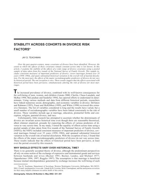
Change in the risk of divorce over time is represented in Figure 1, where the yearly 

proportion of marriages surviving divorce is plotted for the first 10 years of marriage. The 

figure replicates the well-known rise in the risk of divorce that occurred in the 1960s and 

1970s and the slowing of this rise in the 1980s. The change in rates of divorce has been 

substantial. In the 1950–1954 cohort, almost 85% of marriages survived at least 10 years, 

whereas in the last three cohorts, only about 70% of marriages survived at least 10 years. 

MULTIVARIATE RESULTS 

I first ascertained whether the effects of the continuous variables—age at marriage, 

husband’s age at marriage, marriage cohort, and education of husbands and wives—were 

best represented with a continuous coding or a set of dummy variables. I started by 

constructing a set of dummy variables for these variables using the categories presented 

in Table 1. For each of the variables, I then estimated a simple Cox regression model 

using the dummy-variable coding and compared the results with two alternative Cox 

models using the variable coded continuously: a model with only a linear term and a 

model with both a linear and quadratic term. I compared models using both the traditional 

log-likelihood ratio (LR) statistic and Raftery’s (1995) Bayesian information criterion 

(BIC) statistic. 5 

In results not shown, I ascertained that the best-fitting models were those that used a 

linear and a quadratic term for age at marriage, husband’s age at marriage, and marriage 

cohort and a linear term for wife’s education (based on both the LR and BIC statistics). 

For husband’s education, the dummy variables represented a better fit to the data. An 

additional analysis indicated that a dummy variable with three categories for husband’s 

education fit the data best: 12 or fewer years, 13–15 years, and 16 or more years. These 

are the revised codings for the variables that I used in the multivariate analysis. 

I began with a baseline model that includes the additive effect of each variable (Model 

A in Table 2). Based on the weight of prior evidence, the baseline model represents a 

reasonable specification of the effects of the covariates on the risk of divorce. I then tested 

a series of models against this baseline model. Each additional model, except the last, 

includes an interaction between an individual predictor variable and historical time (as 

measured by year of marriage). For example, Model B adds an interaction term between 

age at marriage and year of marriage to the baseline model. Model C then adds an interaction 

term between having a premarital birth and year of marriage to the baseline model, 

and so on. The last model, Model N, includes interactions between all the predictor variables 

and year of marriage. 

Each model with an interaction term was compared with the baseline model via differences 

in the LR and BIC statistics. Although both statistics are presented, I placed 

greater weight on the difference between the BIC statistics to test whether the null hypothesis 

of no interaction should be rejected. I did so because it is well known that conventional 

test statistics are influenced by sample size. Thus, in reasonably large samples, 

such as the one used in this article, it is difficult to reject poor-fitting models using the LR 

statistic. More important, substantively uninteresting differences between models will be 

judged to be statistically significant when sample sizes are large. Thus, even if the baseline 

model is appropriate, use of the LR statistic, in conjunction with a large sample, may 

5. The BIC statistic is calculated as –χ 2 + df × ln(n), where χ 2 is the model chi-square, df is the degrees of 

freedom associated with the model, and n is the number of events (divorces) upon which the model is based. 

Note that I use the number of divorces as the value of n, not the number of marriages, yielding a less conservative 

version of BIC. Models with more negative values of BIC are preferred to models with less negative values 

of BIC. A spirited discussion of the value of BIC as a tool for model selection is provided by Weakliem (1999) 

and the comments to his article in the same issue of Sociological Methods and Research.


Figure 1. Proportion of Marriages Not Disrupted, by Marriage Cohort 

Proportion 

1 

0.95 

0.9 

0.85 

0.8 

0.75 

0.7 

0.65 

1950–1954 

1955–1959 

1960–1964 

1965–1969 

1970–1974 

1975–1979 

1980–1984 

0.6 

0 1 2 3 4 5 6 7 8 9 10 

Marital Duration in Years 

lead to inappropriate conclusions—in this case, to inappropriately reject the null hypothesis 

of simple additive effects in favor of interaction effects. 

The BIC statistic operates by penalizing models when they add degrees of freedom 

or sample size. The procedure is therefore conceptually equivalent to increasing the size 

of a t statistic that is required to reject a null hypothesis for a single coefficient. Although 

there are no formal cutoffs for assessing the importance of a difference between 

two BIC values, Raftery (1995) provided the following guidelines. If there is a difference 

of 10 or more between two BIC values, there is very strong evidence that the null 

model should be rejected. Differences between BIC values of 6–10, 2–6, and 0–2 indicate 

strong, positive, and weak evidence, respectively, that the null model should be 

rejected. In the case of comparisons involving one degree of freedom (e.g., Models B 

through M in Table 2) and the number of divorces in this sample, these values of BIC 

correspond to t values of 3.86–4.35, 3.31–3.86, 2.99–3.31, respectively (squaring these 

values yields the corresponding chi-square values with 1 degree of freedom). Thus, the 

effect of using BIC is simply to require stronger evidence before the null hypothesis of 

no interaction with time is rejected. 

Differences in LR statistics that are significant at p < .05 are presented in italic type. 

Differences in BIC statistics that indicate at least positive support for rejecting the null 

hypothesis (< –2.0) are presented in bold italic type. On the basis of values of the conventional 

LR test statistic, significant interactions involve the husband’s age at marriage and


Table 2. Estimates of Model Fit for Models Involving an Interaction Between Each Predictor 

Variable and Year Married 

Model χ 2 / df BIC 

Model Model χ 2 df Difference BIC Difference 

A: Baseline Additive Model 2,929.58 22 –– –2,732.96 –– 

B: A + Age at Marriage × Year Married 

C: A + Husband’s Age at Marriage × Year 

2,933.14 23 3.56/1 –2,727.58 5.38 

Married 2,938.39 23 8.81/1 –2,732.83 0.13 

D: A + Premarital Birth × Year Married 2,933.14 23 3.56/1 –2,727.58 5.38 

E: A + Premarital Conception × Year Married 2,929.80 23 0.22/1 –2,724.24 8.72 

F: A + Wife Older × Year Married 

G: A + Wife Has More Education × Year 

2,930.51 23 0.93/1 –2,724.95 8.01 

Married 2,931.93 23 2.35/1 –2,726.37 6.59 

H: A + Husband Older × Year Married 2,939.01 23 9.43/1 –2,733.45 –0.49 

I: A + Wife’s Education × Year Married 2,932.22 23 2.64/1 –2,726.66 6.30 

J: A + Husband’s Education × Year Married 2,929.89 24 0.31/2 –2,715.40 17.56 

K: A + Catholic × Year Married 2,936.00 23 6.42/1 –2,731.44 1.52 

L: A + Wife’s Parents Divorced × Year Married 2,931.14 23 1.56/1 –2,725.58 7.38 

M: A + Black × Year Married 2,953.24 23 23.66/1 –2,747.68 –14.72 

N: A + All Interactions With Year Married 2,980.33 35 50.75/13 –2,667.52 65.44 

Notes: All models include a control for survey round. N for the calculation of BIC is 7,611. Values in italic type are 

statistically significant at p < .05. Values in bold italic type show strong evidence using BIC for rejecting the null hypothesis of a 

zero effect. 

the husband being older, being Catholic, and being black. However, the BIC statistic indicates 

only one interaction with positive evidence that the null hypothesis of no change 

across time should be rejected: the effect of being black. 

The results for Model N, which simultaneously includes all interactions with historical 

time, indicate a significantly better-fitting model using the LR statistic but not the 

BIC statistic. Indeed, the substantial increase in the BIC statistic indicates that this model 

may be overparameterized (i.e., may contain too many nonsignificant parameters). The 

individual coefficients from this model, however, are instructive: they indicate that when 

all interactions are considered simultaneously, the only significant interaction, using either 

the LR or BIC statistic as the criterion, is that associated with being black (results 

not shown). This result provides further support for the notion that the only substantial 

interaction with time involves blacks. 

Hazard ratios from bivariate Cox regression models, the additive multivariate baseline 

model (Model A in Table 2), and the model including the interaction between year of 

marriage and being black (Model M in Table 2) are shown in Table 3. The hazard ratios 

shown (e β ) represent multiplicative effects on the hazard of marital dissolution at any 

marital duration. Hazard ratios greater than 1 indicate a positive effect, and hazard ratios 

less than 1 indicate a negative effect. The percentage difference in the risk of divorce at 

any marital duration associated with a unit change in a predictor variable can be calculated 

by subtracting 1 from the hazard ratio and multiplying by 100.


Table 3. Hazard Ratios From Selected Models in Table 2 

Bivariate Model Additive Model Interaction Model 

Variable Coefficients Coefficients Coefficients 

Year Married 1.38 1.41 1.46 

Year Married, Squared 0.97 0.98 0.98 

Age at Marriage 0.63 0.70 0.70 

Age at Marriage Squared 1.01 1.01 1.01 

Husband’s Age at Marriage 0.82 0.92 0.92 

Husband’s Age at Marriage, Squared 1.003 1.001 1.001 

Premarital Birth 2.08 1.68 1.69 

Premarital Conception 1.41 1.16 1.15 

Wife Older 1.48 1.68 1.88 

Wife Has More Education 1.17 1.10a 1.09a Husband Older 1.14 1.19 1.19 

Wife’s Education 0.94 1.04 1.05 

Husband Has 13–15 Years of Schooling 0.59 0.69 0.69 

Husband Has 16+ Years of Schooling 0.39 0.56 0.55 

Catholic 0.69 0.90 0.89 

Wife’s Parents Divorced 1.64 1.39 1.38 

Black 1.99 1.49 1.97 

Black × Year Married –– –– 0.93 

Other Race 0.90b 0.95b 0.93b Note: All models include a control for survey round. 

a 

The null hypothesis that the coefficient is not statistically significant cannot be rejected using a BIC value equal to strong 

evidence (t > 3.31). 

b The coefficient is not statistically significant at the conventional .05 level. 

The hazard ratios for year of marriage and age at marriage are consistent across all 

three models. The coefficients for year of marriage indicate an increasing risk of marital 

dissolution that has slackened in pace more recently. 6 The hazard ratios for each 

spouse’s age at marriage reflect a decrement in the risk of divorce with age that moderates 

somewhat at older ages (although the pattern of change across age at marriage is 

stronger for wives than husbands). 

The effects of both a premarital birth and a premarital conception on divorce are 

positive, with the effect of a premarital birth being much stronger. In both cases, the 

multivariate models show effects that are somewhat lower than in the bivariate model. 

That is, a nontrivial portion of the effect of both variables can be attributed to other 

covariates included in the model. 

6. For the sake of parsimony, I use the phrase “increase or decrease in the risk of divorce” when the 

correct phrase is “increase or decrease in the risk of divorce at a given marital duration.”


The effect of the husband being older on divorce is positive in both the bivariate and 

additive effect models. The effect of the wife being older is substantial. In the interaction 

effect model, if a wife is five or more years older than her husband, the risk of divorce is 

88% higher in comparison with a marriage that has relative age homogamy. The effect of 

the wife having more education is also positive, although not significant using the BIC 

criterion for strong evidence, increasing the risk of divorce by 9% at each marital duration. 

The effect of the wife’s education is interesting in that it reverses direction between 

the bivariate model and the two multivariate models. In the bivariate model, the risk of 

marital disruption decreases 6% for each additional year of schooling the wife has. In the 

multivariate models, the risk of divorce increases 4%–5% for each additional year of the 

wife’s schooling. The switch from a negative to a positive effect is due mostly to the 

inclusion of the control for husband’s education (results not shown). More-educated 

women are generally married to more-educated men, and the effect of the husband’s education 

is substantial and negative. 

The effect of being Catholic is to reduce the risk of marital dissolution, and the effect 

of the wife’s parents having divorced is positive. In both cases, though, the effect is reduced 

somewhat with the introduction of the other covariates. In the interaction model, at 

each marital duration, Catholics are 11% less likely to divorce, and couples in which the 

wives’ parents divorced are 38% more likely to divorce. 

There is no difference between whites and respondents reporting neither white nor 

black race in the risk of marital dissolution. Blacks are substantially more likely to divorce 

at each marital duration than are whites. However, this effect changes across time. 

In the 1950–1954 cohort, the risk of divorce for blacks is 83% greater (1.97 × .93 = 1.83). 

In the 1980–1984 cohort, the risk of marital dissolution for blacks is only 19% higher. 

This pattern results from the fact that the risk of marital dissolution increases more slowly 

(by a factor of .93) for blacks than for whites. 

A Test for Proportionality 

All the models estimated up to this point assume that the effects of the covariates are 

proportional. That is, the effects of the predictor variables are assumed to be equal at all 

marital durations. A test for proportionality is key for the purposes of this study to account 

for the possibility that historical shifts in the risk of divorce may be confused with 

nonproportionality. In particular, a variable with an effect that increases (decreases) with 

marital duration may be mistaken for a variable with an increasing (decreasing) effect 

across historical time. 

In general, two rationales have been put forward to suspect nonproportionality. First, 

as marriages mature, individuals accrue more marital-specific capital (Becker et al. 

1977), decreasing the risk of divorce. Thus, individual couples change with respect to 

their risk of marital disruption. Second, as marriages progress, a process of sorting occurs, 

weeding out couples who are less suited to each other or less committed to a permanent 

relationship (Morgan and Rindfuss 1985; South and Spitze 1986; Teachman 

1986). The remaining marriages are therefore composed of couples who are less likely to 

divorce. 

The empirical evidence is limited, but a number of researchers, using different data 

and methods, have found that the effect of age at marriage is stable across marital duration 

(Morgan and Rindfuss 1985; South and Spitze 1986; Teachman 1986; Thornton and 

Rodgers 1987). Morgan and Rindfuss (1985) reported that the positive effect on divorce 

of having a premarital birth declines at longer marital durations, but Teachman (1986) 

found a more consistent effect for this variable. South and Spitze (1986) and South (2001) 

indicated that the effect of the wife’s education changes from being negative to being 

positive as marriages mature. Again, however, Teachman (1986) found a consistent effect 

of the wife’s education across different marital durations.


Table 4. Tests for the Proportionality of Each of the Predictor Variables 

Model χ 2 / df BIC 

Model Model χ 2 df Difference BIC Difference 

A: Baseline Proportional Effects Model 2,929.58 22 –2,732.97 –– 

B: A + Age at Marriage × Marital Duration 

C: A + Husband’s Age at Marriage × Marital 

2,930.21 23 0.60/1 –2,724.65 8.32 

Duration 2,930.57 23 0.99/1 –2,725.01 7.96 

D: A + Premarital Birth × Marital Duration 

E: A + Premarital Conception × Marital 

2,935.64 23 6.06/1 –2,730.08 2.89 

Duration 2,930.31 23 0.73/1 –2,724.75 8.22 

F: A + Wife Older × Marital Duration 

G: A + Wife Has More Education × Marital 

2,933.91 23 4.33/1 –2,728.35 4.62 

Duration 2,929.60 23 0.02/1 –2,724.04 8.93 

H: A + Husband Older × Marital Duration 2,932.11 23 2.53/1 –2,726.55 6.42 

I: A + Wife’s Education × Marital Duration 2,935.27 23 5.69/1 –2,729.71 3.26 

J: A + Husband’s Education × Marital Duration 2,947.91 24 18.33/2 –2,733.41 –0.44 

K: A + Catholic × Marital Duration 

L: A + Wife’s Parents Divorced × Marital 

2,929.89 23 0.31/1 –2,724.33 8.64 

Duration 2,934.39 23 4.81/1 –2,728.83 4.14 

M: A + Black × Marital Duration 2,934.96 23 5.38/1 –2,729.40 3.57 

Notes: All models include a control for survey round. N for calculating BIC is 7,611. Values in italic type are statistically 

significant at p < .05. 

I tested for the proportionality of effects using a simple interaction between marital 

duration and each of the predictor variables. The results of these tests for proportionality 

are shown in Table 4. I used Model A in Table 2 as the baseline and consider whether the 

addition of nonproportional effects yields a better-fitting model. Again, each model allowing 

nonproportionality was compared with the baseline model via differences in the 

LR and BIC statistics. I continued to attach greater weight to the values of BIC to test 

whether the null hypothesis of proportionality should be rejected. 

Using BIC as the criterion, I found that none of the models allowing for 

nonproportionality yield a better fit to the data than the baseline model. The LR statistic 

suggests nonproportionality for having a premarital birth, the wife being older, the wife’s 

education, the husband’s education, having a wife with divorced parents, and being black. 

With the exception of being black, these are not the same variables for which the LR 

statistics suggested an interaction with historical time. Thus, it is not likely that 

nonproportionality produced these potential interactions with historical time. 

With respect to being black, the nonproportional effect indicates an increasingly positive 

difference across marital duration (result not shown). This pattern strongly suggests 

that nonproportionality is not implicated in the decreasing effect of being black across 

time shown in Table 3. If nonproportionality was involved in producing the changing 

effect of being black across historical time, it would have involved an increasingly negative 

difference across marital duration. 

Finally, I tested for an interaction between year of marriage and marital duration. If 

period effects are present, then the effects of year of marriage should be nonproportional.


Given the rise in the risk of divorce over time, I anticipated that the nature of the interaction 

should be a decreasing effect of year of marriage at longer marital durations (because 

successive marriage cohorts experience a particular marital duration during later periods 

when the risk of divorce is greater). The resulting model (not shown) does fit the data 

better than the baseline model (Model χ 2 = 2,976.54, BIC = –2,770.98). The coefficient 

for the interaction between year of marriage and marital duration is statistically significant 

(using the BIC criterion for strong evidence) and negative (e β = .999). This interaction 

is consistent with the notion that there is a period influence on the risk of marital 

dissolution. Inclusion of this interaction term does not alter the coefficients (or standard 

errors) associated with any of the other covariates. Nor does including this interaction 

term alter any of the findings shown in Tables 2 and 3. 

How Robust Are the Findings? 

I conducted several sensitivity tests to ascertain whether the results are robust to different 

model specifications and restrictions on the data. First, I considered whether different 

results would be obtained if I coded age at marriage and year of marriage as a series of 

dummy variables instead of using continuous variables. Because of the number of potential 

interactions, I estimated a separate model for each interaction between a particular 

age at marriage and year of marriage (using the age at marriage and year of marriage 

categories represented in Table 1). These models do not reveal a pattern of interaction 

between age at marriage and year of marriage that is otherwise masked by using continuous 

variables (see Appendix). 

Second, I considered the possibility that the results may be biased somehow by the 

fact that women who marry in earlier historical periods are more heavily weighted toward 

earlier ages at marriage. To address this issue, I reconfigured the sample and reestimated 

the models using data on marriages formed after 1959. I also formed a sample based on 

all years of marriage but restricted marriages to those formed before age 23, yielding a 

sample in which the maximum age at marriage is consistent across year of marriage. For 

the sample restricted to women who marry before age 23, according to values of the BIC 

statistic, the same interaction as revealed in Table 2 yields a better model fit: the interaction 

of being black with year of marriage (see Appendix). The coefficients from this model 

are similar to those estimated from the full sample. 

In the sample restricted to marriages formed after 1959, the interaction between being 

black and marriage cohort yields weak evidence of a better-fitting model. The important 

point to note from models estimated on this sample, though, is that no new interactions 

appeared when a different set of marriage ages was used. The lack of a substantial 

interaction between being black and year of marriage attests to the need for a long historical 

sequence to detect substantial changes in the risk of divorce. 

Does Cohabitation Make a Difference? 

One substantial change in the nature of intimate relationships has been the sudden and 

steep rise in the incidence and prevalence of premarital cohabitation (Bumpass and Sweet 

1989). Much research has linked premarital cohabitation to an increased risk of marital 

dissolution (Axinn and Thornton 1992; Bumpass, Sweet, and Cherlin 1991; DeMaris and 

MacDonald 1993; Manning and Smock 1994; Thomson and Colella 1992). In this section, 

I seek to answer two questions. First, has the effect of premarital cohabitation on 

divorce changed over time? Second, are the relationships between the measured covariates 

and divorce somehow altered by the substantial increase in premarital cohabitation 

over the past several decades? 

I made use of information on premarital cohabitation contained in rounds 4 and 5 of 

the NSFG, examining marriages formed after 1964. I replicated the models shown in 

Table 2, first using premarital cohabitation as a predictor variable and then excluding


this variable. The results indicated no evidence that the effect of premarital cohabitation 

on the risk of divorce has changed over the relatively short period being considered (see 

Appendix). Nor does the inclusion of cohabitation in any of the models alter the conclusions 

reached about the lack of interaction between the other covariates and historical 

period. Consistent with prior research, the estimated effect of premarital cohabitation 

indicates an increase in the risk of divorce (by about 35%). Also in results not shown, I 

found the effects of premarital cohabitation to be proportional across marital duration. 

Variation in Effects by Race 

I conclude the analysis by estimating models separately for blacks and whites. Not only 

does the effect of race vary by year of marriage, but there is also prior evidence to suggest 

that the effects of various covariates on divorce may differ by race (Martin and 

Bumpass 1989; Teachman 1986). Thus, by estimating models separately by race, I attempted 

to ascertain whether the effects of the measured covariates varied over time differently 

for blacks and whites (results not shown). 

I reestimated the baseline model shown in Table 2 for blacks and whites only. I added 

to the baseline model an interaction between race and year married. The results indicated 

the strong interaction between race and year married indicated in Table 2. I then estimated 

the baseline model separately for blacks and whites, thereby allowing the effects of all the 

covariates to vary according to race. These models were substantially less well fitting than 

a model that constrains the effects of the covariates to be equal across race. Thus, a model 

that allows an interaction between race and year married fits better than the baseline model, 

and a model that allows interactions between race and the remainder of the covariates does 

not fit better. Although it is possible that a smaller subset of covariates may interact with 

race, I did not search for such interactions, given the purposes of this article and the lack of 

otherwise strong theoretical guidance to identify these interactions. 

DISCUSSION 

Using five rounds of the NSFG, I tested for changes in the effects of basic sociodemographic 

variables on the risk of divorce. In the main, most effects have remained constant 

across a period during which rates of divorce varied substantially. The results are robust 

to different model specifications and definitions of the sample. Nor can the results be 

attributed to the nonproportionality of effects across different marital durations. 

Only one clear-cut interaction with historical time was found: that involving the effect 

of race. Specifically, there was a convergence over time in the risk of marital dissolution 

between whites and blacks because the risk of marital dissolution rose more rapidly 

for whites than for blacks. I offer the following interpretation of the interaction between 

race and historical time. Specifically, the declining economic position of many blacks and 

their less favorable marriage-market conditions, when combined with the growth of alternatives 

to marriage and greater acceptance and prevalence of out-of-wedlock childbearing 

and cohabitation, means that blacks who marry are an increasingly select subgroup of 

all blacks. Blacks marry at later ages and are less likely to ever marry than are whites 

(Cherlin 1992; Teachman et al. 2000). Indeed, the environments faced by blacks and 

whites have diverged sufficiently that the current situation is a reversal of historical patterns. 

Before 1950, blacks married earlier than whites and were more likely to have ever 

married (Sweet and Bumpass 1987). Since 1950, blacks have delayed marriage more than 

whites, yielding higher proportions who never marry. 

The result of these changes is that blacks who marry are likely to be selective of 

individuals who are committed to marriage and therefore are less likely to divorce. As a 

consequence, although both blacks and whites have been subject to the pervasive upward 

surge in divorce over the past several decades, the increasing selectivity of blacks into 

marriage has yielded a somewhat slower increase in the risk of marital dissolution.


The changing effect of being black aside, the limited evidence for change in the effects 

of a range of basic sociodemographic predictors of divorce constitutes impressive 

evidence for the pervasive impact of historical period on the risk of marital dissolution. 

For a wide range of variables, there is little evidence of deviation from recent historical 

shifts in divorce. These results mirror the sentiment of Thornton and Rodgers (1987:20) 

that “the degree of uniformity of the historical period effects across population subgroups 

has been remarkable.” 

Although it is important to know that the effects of historical period have been pervasive, 

it still begs the next logical question: what is it about historical periods that 

affects the risk of divorce? This question is all the more important, given the recent 

leveling of divorce rates in the United States (Goldstein 1999), a leveling that cannot be 

explained by compositional factors or the rise in nonmarital cohabitation. There is growing 

evidence, therefore, that marriages are subject to the influence of powerful 

aggregate-level forces that are not yet well understood. Subsequent research should focus 

on identifying and quantifying the characteristics of historical periods that have led 

to such pervasive effects. 

Finally, as a note of caution, I remind readers that there may be other variables not 

considered in the current study that may have effects that vary across time. In particular, 

it would be beneficial for subsequent research to consider the impact of a wider range of 

variables that may be more tightly linked to the instrumental and expressive exchange 

that occurs between spouses. For example, more information about changes in the influence 

of variables, such as wives’ labor force participation, occupations, and gender-role 

ideology and the division of household labor, could provide additional evidence about 

the nature of period effects on marital dissolution. On the basis of the exchange model, 

South (2001) outlined good reasons for expecting the effect of wives’ labor force participation 

on divorce to change across time, and his empirical results suggest an effect that 

has become increasingly positive. South’s findings indicate the complexity of factors 

that influence divorce and argue for care in specifying the components of marriage that 

may be important to marital stability in a particular context. Although there is evidence 

that a wide range of important risk factors have consistent effects on divorce over time, 

the changing nature and context of marital unions argues for the continued investigation 

of a wider range of factors that can be linked to marital cohesion.


Appendix Table A1. Estimates of Model Fit for Various Sensitivity Models 

____________________________________________________ ____________________________________________________ 

Marriages Formed After 1959 Marriages Formed Before Age 23 

Model χ2 / df BIC Model χ2 / df BIC 

Model Model χ2 df Difference BIC Difference Model χ2 df Difference BIC Difference 

A: Baseline Additive Model 2,056.08 22 –1,864.82 –– 2,476.85 22 –2,283.53 

B: A + Age at Marriage × Year 

Married 2,057.55 23 1.47/1 –1,856.76 8.06 2,480.60 23 3.75/1 –2,278.48 5.05 

C: A + Husband’s Age at Marriage 

× Year Married 2,059.13 23 3.05/1 –1,858.34 6.48 2,482.13 23 5.28/1 –2,280.02 3.51 

C: A + Premarital Birth × Year 

Married 2,060.83 23 4.75/1 –1,860.05 4.77 2,481.01 23 4.16/1 –2278.90 4.63 

D: A + Premarital Conception 

× Year Married 2,056.20 23 0.12/1 –1,855.41 9.41 2,477.07 23 0.22/1 –2,274.96 8.63 

E: A + Wife Older × Year Married 2,056.24 23 0.16/1 –1,855.45 9.37 2,478.44 23 1.59/1 –2,276.33 3.86 

F: A + Wife Has More Education 

× Year Married 2,061.30 23 5.22/1 –1,860.51 4.31 2,481.61 23 4.76/1 –2,279.50 4.03 

G: A + Husband Older × Year 

Married 2,062.50 23 6.92/1 –1,861.71 2.91 2,487.12 23 10.27/1 –2,285.01 –1.48 

H: A + Wife’s Education × Year 

Married 2,056.15 23 0.70/1 –1,855.37 9.45 2,478.96 23 2.11/1 –2,276.85 6.68 

I: A + Husband’s Education 

× Year Married 2,057.85 24 1.77/2 –1,848.33 16.49 2,477.51 24 0.66/2 –2,266.61 16.92 

K: A + Catholic × Year Married 2,060.55 23 4.47/1 –1,859.76 5.06 2,481.47 23 4.62/1 –2,279.36 4.17 

L: A + Wife’s Parents Divorced 

× Year Married 2,056.88 23 0.80/1 –1,856.09 8.73 2,477.57 23 0.72/1 –2,275.46 8.07 

M: A + Black × Year Married 2,066.44 23 10.36/1 –1,865.65 –0.83– 2,498.08 23 21.23/1 –2,295.97 –12.44 

Notes: All models include a control for survey round. N for calculating BIC for marriages formed after age 1959 is 6,185. N for calculating BIC for marriages formed before age 23 is 6,551. 

Values in italic type are statistically significant at p < .05. Values in bold italic type show strong evidence using BIC for rejecting the null hypothesis of a zero effect.


Appendix Table A2. Estimates of Model Fit for Models Including and Then Excluding Cohabitation 

____________________________________________________ ____________________________________________________ 

Including Premarital Cohabitation Excluding Premarital Cohabitation 

Model χ2 / df BIC Model χ2 / df BIC 

Model Model χ2 df Difference BIC Difference Model χ2 df Difference BIC Difference 

A: Baseline Additive Model 869.36 20 –709.19 –– 824.55 19 –672.39 –– 

B: A + Age at Marriage × Year 

Married 869.86 21 0.50/1 –701.69 7.50 824.84 20 0.29/1 –664.67 7.72 

C: A + Husband’s Age at Marriage 

× Year Married 872.56 21 3.20/1 –704.38 4.81 827.48 20 2.93/1 –667.31 4.99 

D: A + Premarital Birth × Year 

Married 869.60 21 0.24/1 –701.42 7.77 824.95 20 0.40/1 –664.78 7.52 

E: A + Premarital Conception 

× Year Married 870.87 21 1.27/1 –702.70 6.49 826.24 20 1.69/1 –666.07 6.23 

F: A + Wife Older × Year Married 869.40 21 0.04/1 –701.22 7.97 824.58 20 0.03/1 –664.41 7.89 

G: A + Wife Has More Education 

× Year Married 869.36 21 0.00/1 –701.18 8.01 824.55 20 0.00/1 –664.38 8.01 

H: A + Husband Older × Year 

Married 869.64 21 0.28/1 –701.46 7.73 824.76 20 0.21/1 –664.59 7.71 

I: A + Wife’s Education × Year Married 870.42 21 1.05/1 –702.25 6.94 825.62 20 1.07/1 –665.45 6.85 

J: A + Husband’s Education × Year 

Married 875.93 22 6.57/2 –699.75 9.44 831.21 21 6.66/2 –663.04 9.26 

L: A + Catholic × Year Married 870.71 21 1.35/1 –702.54 6.65 826.05 20 1.50/1 –665.88 6.42 

M: A + Wife’s Parents Divorced 

× Year Married 869.43 21 0.07/1 –701.25 7.94 824.78 20 0.23/1 –664.61 7.69 

N: A + Premarital Cohabitation 

× Year Married 871.94 21 2.58/1 –703.77 5.42 –– –– –– –– –– 

O: A + Black × Year Married 870.67 21 1.31/1 –702.50 6.69 826.33 20 1.78/1 –666.16 6.14 

Notes: All models include a control for survey round. N for estimating BIC is 3,006. Values in italic type are statistically significant at p < .05.


REFERENCES 

Allison, P. 1995. Survival Analysis Using the SAS System: A Practical Guide. Cary, NC: SAS Institute. 

Amato, P. 2000. “The Consequences of Divorce for Adults and Children.” Journal of Marriage 

and the Family 62:1269–87. 

Axinn, W. and A. Thornton. 1992. “The Relationship Between Cohabitation and Divorce: Selectivity 

or Causal Influence.” Demography 29:357–74. 

Becker, G. 1991. A Treatise on the Family. Cambridge, MA: Harvard University Press. 

Becker, G., E. Landes, and R. Michael. 1977. “An Economic Analysis of Marital Instability.” Journal 

of Political Economy 85:1141–87. 

Bianchi, S. 1995. “Changing Economic Roles of Women and Men.” Pp. 107–54 in State of the 

Union: America in the 1990s, Vol. 1: Economic Trends, edited by R. Farley. New York: Russell 

Sage Foundation. 

Booth, A. and J. Edwards. 1985. “Age at Marriage and Marital Instability.” Journal of Marriage 

and the Family 47:67–75. 

Bumpass, L., T. Martin, and J. Sweet. 1991. “The Impact of Family Background and Early Marital 

Factors on Marital Disruption.” Journal of Family Issues 12:22–42. 

Bumpass, L. and J. Sweet. 1972. “Differentials in Marital Instability: 1970.” American Sociological 

Review 37:754–66. 

———. 1989. “National Estimates of Cohabitation.” Demography 26:615–25. 

Bumpass, L., J. Sweet, and A. Cherlin. 1991. “The Role of Cohabitation in Declining Rates of 

Marriage.” Journal of Marriage and the Family 53:913–27. 

Carlson, E. and K. Stinson. 1982. “Motherhood, Marriage Timing, and Marital Stability.” Social 

Forces 61:258–67. 

Cherlin, A. 1992. Marriage, Divorce, Remarriage, rev. ed. Cambridge, MA: Harvard University 

Press. 

Cherlin, A., P. Chase-Lansdale, and C. McRae. 1998. “Effects of Parental Divorce and Mental 

Health Throughout the Life Course.” American Sociological Review 63:239–49. 

Clarkberg, M., R. Stolzenberg, and L. Waite. 1995. “Attitudes, Values, and Entrance Into 

Cohabitational Versus Marital Unions.” Social Forces 74:609–34. 

Coley, R. and P. Chase-Lansdale. 1998. “Adolescent Pregnancy and Parenthood: Recent Evidence 

and Future Directions.” American Psychologist 53:152–66. 

Cox, D. 1972. “Regression Models With Life Tables.” Journal of the Royal Statistical Society 

B34:187–220. 

DaVanzo, J. and M. Rahman. 1993. “American Families: Trends and Correlates.” Population Index 

59:350–86. 

DeMaris, A. and W. MacDonald. 1993. “Premarital Cohabitation and Marital Instability: A Test of 

the Unconventionality Hypothesis.” Journal of Marriage and the Family 55:399–407. 

Ellwood, D. and J. Crane. 1990. “Family Change Among African-Americans: What Do We Know?” 

Journal of Economic Perspectives 4:65–84. 

Eysenck, H. 1980. “Personality, Marital Satisfaction, and Divorce.” Psychological Reports 

47:1235–38. 

Faust, K. and J. McKibben. 1999. “Marital Dissolution: Divorce Separation, Annulment, and Widowhood.” 

Pp. 475–99 in Handbook of Marriage and the Family, 2nd ed., edited by M. Sussman, 

S. Steinmetz, and G. Peterson. New York: Plenum. 

Goldstein, J. 1999. “The Leveling of Divorce in the United States.” Demography 36:409–14. 

Heaton, T. 1991. “Time Related Dimensions of Marital Dissolution.” Journal of Marriage and the 

Family 53:285–95. 

Jockin, V., M. McGue, and D. Lykken. 1996. “Personality and Divorce: A Genetic Analysis.” Journal 

of Personality and Social Psychology 71:288–99. 

Johnson, J. and W. Harris. 1980. “Personality and Behavioral Characteristics Related to Divorce in


a Population of Male Applicants for Psychiatric Evaluation.” Journal of Abnormal Psychology 

89:510–13. 

Kiernan, K. 1986. “Teenage Marriage and Marital Breakdown: A Longitudinal Study.” Population 

Studies 40:35–54. 

Lehrer, E. and C. Chiswick. 1993. “Religion as a Determinant of Marital Stability.” Demography 

30:385–404. 

Lichter, D., F. LeClere, and D. McLaughlin. 1991. “Local Marriage Markets and the Marital Behavior 

of African American and White Women.” American Journal of Sociology 96:843–67. 

Lichter, D., D. McLaughlin, G. Kephart, and D. Landry. 1992. “Race and the Retreat From Marriage: 

A Shortage of Marriageable Men?” American Sociological Review 57:781–99. 

Manning, W. and P. Smock. 1995. “Why Marry? Race and the Transition to Marriage Among Cohabitors.” 

Demography 32:509–20. 

Martin, T. and L. Bumpass. 1989. “Recent Trends in Marital Disruption.” Demography 26:37–51. 

McGue, M. and D. Lykken. 1992. “Genetic Influence on Risk of Divorce.” Psychological Science 

6:368–73. 

McLanahan, S. and L. Casper. 1995. “Growing Diversity and Inequality in the American Family.” 

Pp. 1–45 in State of the Union: America in the 1990s, Vol. 2, edited by R. Farley. New York: 

Russell Sage Foundation. 

McLanahan, S. and G. Sandefur. 1994. Growing Up With a Single Parent: What Hurts, What Helps. 

Cambridge, MA: Harvard University Press. 

Morgan, S. and R. Rindfuss. 1985. “Marital Disruption: Structural and Temporal Dimensions.” 

American Journal of Sociology 90:1055–77. 

———. 1999. “Reexamining the Link of Early Childbearing to Marriage and to Subsequent Fertility.” 

Demography 36:59–75. 

National Center for Health Statistics. 1998. “National Survey of Family Growth (NSFG) Public- 

Use Data Files.” Available on-line at http://www.cdc.gov/nchswww/products/catalogs/subject/ 

nsfg/nsfg.htm. 

Ono, H. 1999. “Historical Time and Marital Dissolution.” Social Forces 77:969–97. 

Oppenheimer, V.K. 1994. “Women’s Rising Employment and the Future of the Family in Industrialized 

Societies.” Population and Development Review 20:293–342. 

———. 1997. “Women’s Employment and the Gain to Marriage: The Specialization and Trading 

Model.” Annual Review of Sociology 23:431–53. 

Plotnick, R. 1992. “The Effects of Attitudes on Teenage Premarital Pregnancy and Its Resolution.” 

American Sociological Review 57:800–11. 

Raftery, A. 1995. “Bayesian Model Selection in Social Research.” Pp. 111–63 in Sociological Methodology, 

edited by P. Marsden. Washington DC: American Sociological Association. 

Rockwell, R., G. Elder, and D. Ross. 1979. “Psychological Patterns in Marital Timing and Divorce.” 

Social Psychology Quarterly 42:399–404. 

Ruggles, S. 1997. “The Rise of Divorce and Separation in the United States, 1880–1990.” Demography 

34:455–66. 

Schoen, R. 1992. “First Union and the Stability of First Marriage.” Journal of Marriage and the 

Family 54:281–84. 

South, S. 1999. “Historical Changes and Life Course Variations in the Determinants of Premarital 

Childbearing.” Journal of Marriage and the Family 61:752–63. 

———. 2001. “Time-Dependent Effects of Wives’ Employment on Marital Dissolution.” American 

Sociological Review 66:226–45. 

South, S. and K. Lloyd. 1995. “Spousal Alternatives and Marital Dissolution.” American Sociological 

Review 60:21–35. 

South, S. and G. Spitze. 1986. “Determinants of Divorce Over the Marital Life Course.” American 

Sociological Review 51:583–90. 

Sweet, J. and L. Bumpass. 1987. American Families and Households. New York: Russell Sage 

Foundation.


Teachman, J. 1986. “First and Second Marital Dissolution: A Decomposition Exercise for Whites 

and Blacks.” Sociological Quarterly 27:571–90. 

———. 2000. “Diversity of Family Structure: Economic and Social Influences.” Pp. 32–58 in 

Handbook of Family Diversity, edited by D. Demo, K. Allen, and M. Fine. New York: Oxford 

University Press. 

Teachman, J. and K. Polonko. 1980. “Cohabitation and Marital Stability in the United States.” 

Social Forces 69:207–20. 

Teachman, J., L. Tedrow, and K. Crowder. 2000. “The Changing Demography of America’s Families.” 

Journal of Marriage and the Family 62:1234–46. 

Thomson, E. and U. Colella. 1992. “Cohabitation and Marital Stability: Quality or Commitment?” 

Journal of Marriage and the Family 54:259–67. 

Thornton, A. 1989. “Changing Attitudes Toward Family Issues in the United States.” Journal of 

Marriage and the Family 51:873–93. 

Thornton, A. and W. Rodgers. 1987. “The Influence of Individual and Historical Time on Marital 

Dissolution.” Demography 24:1–22. 

Turkheimer, E., G. Lovett, C. Robinette, and I. Gottesman. 1992. “The Heritability of Divorce: 

New Data and Theoretical Implications.” Paper presented at the annual meeting of the Behavioral 

Genetics Association, Boulder, CO. 

Waite, L. and L. Lillard. 1991. “Children and Marital Disruption.” American Journal of Sociology 

96:930–53. 

Weakliem, D. 2001. “A Critique of the Bayesian Information Criterion in Model Selection.” Sociological 

Methods and Research 27:359–97. 

White, L. 1990. “Determinants of Divorce: A Review of Research in the Eighties.” Journal of 

Marriage and the Family 52:904–12. 

Wolfinger, N. 1999. “Trends in the Intergenerational Transmission of Divorce.” Demography 

36:415–20.

Stability Across Cohorts in Divorce Risk Factors - Bishop Ireton High ...

You also want an ePaper? Increase the reach of your titles

Delete template?

Save as template?