Gasoline Price Changes - Federal Trade Commission

Federal Trade Commission 

DEBORAH PLATT MAJORAS Chairman 

ORSON SWINDLE Commissioner 

THOMAS B. LEARY Commissioner 

PAMELA JONES HARBOUR Commissioner 

JON LEIBOWITZ Commissioner 

Maryanne Kane Chief of Staff 

Charles H. Schneider Executive Director 

Susan A. Creighton Director, Bureau of Competition 

Lydia B. Parnes Director, Bureau of Consumer Protection 

Luke Froeb Director, Bureau of Economics 

William Blumenthal General Counsel 

Anna H. Davis Director, Office of Congressional Relations 

Nancy Ness Judy Director, Office of Public Affairs 

Maureen K. Ohlhausen Director, Office of Policy Planning 

Donald S. Clark Secretary of the Commission 

Report Drafters and Contributors 

Louis Silvia, Assistant Director, Bureau of Economics 

David Meyer, Bureau of Economics 

Sarah M. Mathias, Office of General Counsel Policy Studies 

Michael S. Wroblewski, Assistant General Counsel Policy Studies 

Phillip L. Broyles, Assistant Director, Bureau of Competition 

J. Elizabeth Callison, Bureau of Economics 

Jeffrey Fischer , Bureau of Economics 

Nicolas J. Franczyk, Bureau of Competition 

Daniel E. Gaynor, Bureau of Economics 

Geary A. Gessler, Bureau of Economics 

James F. Mongoven, Bureau of Competition 

John H. Seesel, Associate General Counsel for Energy 

Christopher T. Taylor, Bureau of Economics 

Michael G. Vita, Assistant Director, Bureau of Economics 

Anthony G. Alcorn, Bureau of Economics 

Sarah Croake, Bureau of Competition 

Madeleine McChesney, Bureau of Economics 

Guru Raj, Bureau of Competition 

Natalie Shonka, Office of General Counsel Policy Studies 

Inquiries concerning this report should be directed to: 

John H. Seesel at (202) 326-2702 or jseesel@ftc.gov 

Sarah M. Mathias (202) 326-3254 or smathias@ftc.gov. 

Acknowledgments: 

The FTC appreciates the expertise and time contributed by Hearings participants. 

For all of their contributions, the FTC conveys its thanks.

EXECUTIVE SUMMARY 

Many people who purchased gasoline in the U.S. in the past week likely could report the 

price paid per gallon. Consumers closely follow gasoline prices, and with good reason. U.S. 

consumers have experienced dramatic increases and wide fluctuations in gasoline prices over the 

past several years. During 2004 and 2005, U.S. consumers spent millions of dollars more on 

gasoline than they had anticipated. In the spring of 2005, the national weekly average price of 

gasoline at the pump, including taxes, rose as high as $2.28 per gallon. Steep, but temporary, 

gasoline price spikes have occurred in various areas throughout the U.S. Since the mid-1990s, 

consumers on the West Coast, especially in California, have observed that their gasoline prices 

are usually higher than elsewhere in the U.S. 

Rising average gasoline prices and gasoline price spikes command our attention. What 

causes high gasoline prices like those of 2004 and 2005? What causes gasoline price spikes? 

These important questions require a thorough and accurate analysis of the factors – supply, 

demand, and competition, as well as federal, state, and local regulations – that drive gasoline 

prices, so that policymakers can evaluate and choose strategies likely to succeed in addressing 

high gasoline prices. 

This Report provides such an analysis, drawing upon what the Federal Trade 

Commission (FTC) has learned about the factors that can influence average gasoline prices or 

cause gasoline price spikes. Over the past 30 years, the FTC has investigated nearly all oilrelated 

antitrust matters and has held public hearings, undertaken empirical economic studies, 

and prepared extensive reports on oil-related issues, such as the Midwest gasoline price spike in 

June 2000. Since 2002, the staff of the FTC has monitored weekly average retail gasoline and 

diesel prices in 360 cities nationwide to find and, if necessary, recommend appropriate action on 

pricing anomalies that might indicate anticompetitive conduct. 

Some observers suggest that oil company collusion, anticompetitive mergers, or other 

anticompetitive conduct – not market forces – may be the primary cause of higher gasoline 

prices. Anticompetitive conduct is always a possibility, of course. That is the reason for the 

antitrust laws. The FTC has been and remains vigilant regarding anticompetitive conduct in this 

industry. The FTC has taken action against proposed mergers in this industry at concentration 

levels lower than in other industries. Since 1981, the FTC has investigated 16 large petroleum 

mergers. In 12 of these cases, the FTC obtained significant divestitures and in the four other 

cases, the parties abandoned the transactions altogether after antitrust challenge. In 2004, the 

FTC staff published a study reviewing the petroleum industry’s mergers and structural changes 

as well as the antitrust enforcement actions the FTC has taken. 1 In no other industry does the 

FTC maintain a price monitoring project such as its project to monitor retail gasoline and diesel 

prices. Most recently, on June 10, 2005, the FTC announced the acceptance of two consent 

orders that resolved the competitive concerns relating to Chevron’s acquisition of Unocal and 

settled the FTC’s 2003 monopolization complaint against Unocal. The Unocal settlement alone 

has the potential of saving consumers nationwide billions of dollars in future years. 2

GASOLINE PRICE CHANGES: 

The vast majority of the FTC’s investigations have revealed market factors to be the 

primary drivers of both price increases and price spikes. This Report describes the complex 

landscape of market forces that affect gasoline prices in the U.S. 

The Report does not suggest or evaluate strategies for addressing high gasoline prices. 

Rather, the Report provides an empirical analysis to help policymakers evaluate different 

proposals to address high gasoline prices and consumers understand the reasons for gasoline 

price changes. 

I. A CASE EXAMPLE TEACHES THREE BASIC LESSONS. 

In August 2003, the FTC staff observed anomalous retail gasoline prices in Phoenix, 

Arizona. At the beginning of August 2003, the average price of gasoline in Phoenix was $1.52 

per gallon. By the third week of August, however, it had peaked at $2.11 per gallon. Over the 

next few weeks, the price dropped, falling to $1.80 per gallon by the end of September. 

The price spike was caused by a pipeline rupture on July 30, and the failure of temporary 

repairs, which had reduced the volume of gasoline supplies to Phoenix by 30 percent from 

August 8 through August 23. Arizona has no refineries. It obtains gasoline primarily through 

two pipelines, one traveling from west Texas and the other from the West Coast. The rupture 

closed the portion of the Texas line between Tucson and Phoenix. 

The shortage of gasoline supplies in Phoenix caused gasoline prices to increase sharply. 

To obtain additional supply, Phoenix gas stations had to pay higher prices to West Coast 

refineries than West Coast gas stations were paying. West Coast refineries responded by selling 

more of their supplies to the Phoenix market. 

Phoenix consumers did not respond to significantly increased gasoline prices with 

substantial reductions in the amount of gasoline they purchased. In theory, to prevent a gasoline 

price hike, Phoenix consumers could have reduced their gasoline purchases by 30 percent. 

Without price increases, however, consumers do not have incentives to change the amount of 

gasoline they buy. Moreover, even with price increases, most consumers do not respond to 

short-term supply disruptions such as a pipeline break by making the types of major changes – 

the car they drive, their driving habits, where they live, or where they work – that could 

substantially reduce the amount of gasoline they consume. 

At some point, gasoline prices can become high enough that consumers will make 

substantial reductions in their gasoline purchases. How much prices need to increase depends on 

how easily consumers can adopt substitutes for gasoline – such as taking public transportation. 

Empirical studies indicate that consumers do not easily find substitutes for gasoline, and that 

prices must increase significantly to cause even a relatively small decrease in the quantity of 

gasoline consumers want. In the short run, a gasoline price increase of 10 percent would reduce 

consumer demand by just 2 percent, according to these studies. This suggests that gasoline 

prices in Phoenix would have had to increase by a large amount to reduce the quantity of 

ii 

FEDERAL TRADE COMMISSION, JUNE 2005

THE DYNAMIC OF SUPPLY, DEMAND, AND COMPETITION 

consumers’ purchases by 30 percent, the amount of lost supply. Extrapolating from above, 

prices would have to increase by 150 percent. 3 Phoenix prices did increase substantially – by 40 

percent – but remained far below a 150 percent price increase, because Phoenix gas stations had 

succeeded in obtaining some additional gasoline supplies from the West Coast. This new supply 

of gasoline dampened price increases to some extent. 

On August 24, the pipeline owner restarted gasoline flow on the Tucson-Phoenix line, 

although at a reduced capacity. Retail gasoline prices in Phoenix declined by about $0.31 per 

gallon between the last week in August and the end of September. Phoenix gas stations, 

however, still had to obtain significant quantities of gasoline from West Coast refineries by 

pipeline or from other terminals by truck – both at higher cost. 

Three basic lessons emerge from this example. 

First, in general, the price of a commodity, such as gasoline, reflects producers’ costs and 

consumers’ willingness to pay. Gasoline prices rise if it costs more to produce and supply 

gasoline, or if people wish to buy more gasoline at the current price – that is, when demand is 

greater than supply. Gasoline prices fall if it costs less to produce and supply gasoline, or if 

people wish to buy less gasoline at the current price – that is, when supply is greater than 

demand. Gasoline prices will stop rising or falling when they reach the price at which the 

quantity consumers demand matches the quantity that producers will supply. In Phoenix, prices 

rose primarily because there was not enough gasoline to supply the quantity demanded at the 

prices that prevailed before the pipeline broke. 

Second, how consumers respond to price changes will affect how high prices rise and 

how low they fall. Limited substitutes for gasoline restrict the options available to consumers to 

respond to price increases. That gasoline consumers typically do not reduce their purchases 

substantially in response to price increases makes them vulnerable to substantial price increases, 

such as the 40 percent price increase in Phoenix. 

Third, how producers respond to price changes will affect how high prices rise and how 

low they fall. In general, when there is not enough of a product to meet consumers’ demands at 

current prices, higher prices will signal a potential profit opportunity and may bring additional 

supply into the market. How high prices have to be to bring in additional supply will depend on 

how costly it is for producers to expand output. Phoenix gas stations’ offers to pay prices to 

West Coast refiners that were higher than they had been receiving from West Coast gas stations 

were sufficient to bring additional supplies into Phoenix. 

II. WORLDWIDE SUPPLY, DEMAND, AND COMPETITION FOR CRUDE OIL 

ARE THE MOST IMPORTANT FACTORS IN THE NATIONAL AVERAGE 

PRICE OF GASOLINE IN THE U.S. 

To understand U.S. gasoline prices over the past three decades, including why gasoline 

prices rose so high and so sharply in 2004 and 2005, we must begin with crude oil. 

EXECUTIVE SUMMARY iii


$ The World Price of Crude Oil Is the Most Important Factor in the Price of Gasoline. 

Over the Last 20 Years, Changes in Crude Oil Prices Have Explained 85 Percent of the 

Changes in the Price of Gasoline in the U.S. 

U.S. refiners compete with refiners all around the world to obtain crude oil. Refiners in 

the U.S. now import more than 60 percent of their crude from foreign sources, up from 43 

percent in 1978. The prices of crude oil produced and sold domestically also are linked to world 

crude prices. 

If world crude prices rise, then U.S. refiners must offer and pay higher prices for crude 

they buy. Facing higher input costs from crude, refiners charge more for the gasoline they sell at 

wholesale. This requires gas stations to pay more for their gasoline. In turn, gas stations, facing 

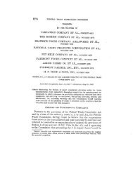
higher input costs, charge consumers more at the pump. To illustrate this relationship, Figure 2- 

1 compares the U.S. annual average price of gasoline (excluding taxes) with the annual average 

price of a recognized crude oil benchmark, West Texas Intermediate (WTI), from 1984 to 

January 2005. 4 When crude oil prices rise, gasoline prices rise because gasoline becomes more 

costly to produce. 

iv 

Price (Cents per Gallon) 

200 

180 

160 

140 

120 

100 

80 

60 

40 

20 

0 

1/1/1984 

Source: EIA 

Figure 2-1: Comparison of the National Average Price of Gasoline and the Price of 

West Texas Intermediate Crude (1984-Jan. 2005) 

1/1/1985 

1/1/1986 

National Gasoline Average (Excluding Taxes) 

WTI Crude 

1/1/1987 

1/1/1988 

1/1/1989 

1/1/1990 

1/1/1991 

1/1/1992 

1/1/1993 

Gasoline Price 

(Left Axis) 

Crude Oil Price 

(Right Axis) 

) 

1/1/1994 

1/1/1995 

1/1/1996 

1/1/1997 

1/1/1998 

1/1/1999 

1/1/2000 

1/1/2001 

1/1/2002 

1/1/2003 

1/1/2004 

1/1/2005 

60 

50 

40 

30 

20 

10 

0 

Price (Dollars per Barrel) 



$ Since 1973, Production Decisions by OPEC Have Been a Very Significant Factor in the 

Prices That Refiners Pay for Crude Oil. 

The Organization of Petroleum Exporting Countries (OPEC) is a cartel designed 

specifically to coordinate output decisions and to affect world crude oil prices. 5 Beginning with 

OPEC’s first successful assertion of market power in 1973-1974, market forces no longer were 

the sole determinant of the world price of crude oil. At that time, OPEC members agreed to limit 

how much crude oil they would produce and to embargo the sale of crude oil to the U.S. OPEC 

members adhered to the production limits and, when OPEC lifted the embargo six months later, 

crude oil prices had tripled from $4 to $12 per barrel. 

The degree of OPEC’s success in raising crude oil prices has varied over time. OPEC 

members can be tempted to “cheat” and sometimes sell more crude oil than specified by OPEC 

limits. Higher world crude prices due to OPEC’s actions increased the incentives to search for 

oil in other areas, and crude supplies from non-OPEC members such as Canada, the United 

Kingdom, and Norway have increased significantly. In 2003, almost 30 years after the first oil 

embargo, OPEC’s total crude production was about the same as in 1974, but accounted for only 

38 percent of world crude production, as compared to 52 percent of world crude oil production in 

1974. Another countervailing force against higher crude prices has been new technologies that 

aid in finding new oil fields and lowering extraction costs. 

Nonetheless, OPEC still produces a large enough share of world crude oil to exert market 

power and strongly influence the price of crude oil when OPEC members adhere to their 

assigned production quotas. Especially when demand surges unexpectedly, as in 2004, OPEC 

decisions on whether to increase supply to meet demand can have a significant impact on world 

crude oil prices. 

$ Over the Past Two Decades, the Demand for Crude Oil Has Grown Significantly. 

The demand for crude oil depends on the demand for refined products, such as gasoline, 

diesel fuel, jet fuel, and heating oil. Since 1982, gasoline has accounted for 49 to 53 percent of 

the daily consumption of all petroleum products. Crude oil consumption has fallen during some 

periods over the past 30 years, partially in reaction to higher prices and federal laws such as 

requirements to increase the fuel efficiency of cars. Gasoline consumption in the U.S. fell 

significantly between 1978 and 1982, and remained lower during the 1980s than it had been at 

the beginning of 1978. See Figure 3-6, supra. 

Overall, however, the long-run trend is toward significantly increased demand for crude 

oil. Over the last 20 years, average daily U.S. consumption of all refined petroleum products 

increased on average by 1.5 percent per year, leading to a total increase of 30 percent. As a 

result, worldwide demand for crude increased by 27 percent between 1988 and 2004. One would 

EXECUTIVE SUMMARY v


expect increased demand for crude oil at current prices to produce crude oil price increases. 

Throughout most of the 1990s, however, crude prices remained relatively stable, suggesting that 

crude producers increased production to meet increased demand. See Figure 3-6, supra. 

$ In 2004, Crude Producers Were Unprepared to Produce Enough Crude Oil to Meet 

Larger-than-Predicted Increases in World Demand. Crude Oil Prices Increased Because 

There Was Not Enough Crude Supply to Meet Increasing Demand at Previous Price 

Levels. Steep Increases in World Prices for Crude Oil Caused Steep Increases in 

Gasoline Prices. 

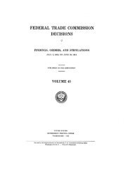
Crude oil producers had set 2004 production levels based on much lower projections for 

demand growth than actually occurred. Projections had placed likely growth in world demand 

for crude oil at 1.5 percent. In fact, the 2004 rate of growth in crude demand was more than 

double the projections: 3.3 percent. See Figure 2-6. Large demand increases from rapidly 

industrializing countries, particularly China and India, made supplies much tighter than expected. 

This phenomenon was not limited to crude oil. Other commodities that form the basis for 

expanded growth in developing economies, such as steel and lumber, also saw unexpectedly 

rapid growth in demand, along with higher prices. 

Million Barrels per Day 

0.9 

0.8 

0.7 

0.6 

0.5 

0.4 

0.3 

0.2 

0.1 

0.0 

-0.1 

Source: IEA 

Figure 2-6: 2004 Predicted vs. Actual Crude Oil Demand Increase, 


Predicted Demand Increase 

Actual Demand Increase 

US Other North 

America 

Europe China Other Asia 

(inc. India) 

Country or Region 

Middle East Latin 

America 

Rest of 

World 

In addition, unexpected production difficulties reduced some producers’ crude output, putting 

upward pressure on prices. Finally, the 2004 political outlook in certain regions, including 

prospects for terrorist incidents or civil unrest, appeared to threaten the production capacity of 

vi 



some major oil producers. For the most part, production actually did not decrease significantly 

in any of the areas of concern. However, even incidents that do not directly affect current crude 

oil production can create concerns and fears about potential crude supply disruptions and thus 

contribute to increases in crude spot and futures prices. 

III. GASOLINE SUPPLY, DEMAND, AND COMPETITION PRODUCED 

RELATIVELY LOW AND STABLE ANNUAL AVERAGE REAL U.S. 

GASOLINE PRICES FROM 1984 UNTIL 2004, DESPITE SUBSTANTIAL 

INCREASES IN U.S. GASOLINE CONSUMPTION. 

A review of annual average U.S. gasoline prices in real terms over the past decades 

reveals surprisingly low prices. Despite ever-growing gasoline consumption in the U.S., 

increased gasoline supply from U.S. refiners and imports, as well as relatively stable crude oil 

prices, kept U.S. gasoline prices in check throughout the 1990s. These prices reflect national 

averages that do not capture regional differences, to be discussed in the succeeding section. Yet 

they provide an important historical perspective on gasoline prices over the past 20 years. 

$ U.S. Consumer Demand for Gasoline Has Risen Substantially, Especially Since 1990. 

In 1978, U.S. gasoline consumption was about 7.4 million barrels per day. By 1981, in 

the face of sharply escalating crude oil and gasoline prices and a recession, U.S. gasoline 

consumption had fallen by roughly a million barrels per day, averaging about 6.5 million barrels 

per day. As gasoline prices began to fall in the 1980s, U.S. consumption of gasoline began to 

rise once again. In 1993, U.S. gasoline consumption rose above 1978 levels; it has continued to 

increase at a fairly steady rate since then. In 2004, U.S. gasoline consumption averaged about 9 

million barrels per day. U.S. gasoline consumption continues to rise, with the U.S. Energy 

Information Administration (EIA) forecasting 2005 demand at an average of 9.2 million barrels 

per day. 

$ Increased Gasoline Supply from U.S. Refineries and Imports Helped to Meet Increased 

U.S. Demand for Gasoline and Keep Gasoline Prices Relatively Steady. 

A comparison of “real” average annual retail gasoline prices and average annual retail 

gasoline consumption in the U.S. from 1978 through 2004 shows that, in general, gasoline prices 

remained relatively stable despite significantly increased demand. See Figure 3-6. “Real” prices 

are adjusted for inflation and therefore reflect the different values of a dollar at different times; 

they provide more accurate comparisons of prices in different time periods. “Nominal” prices 

are the literal prices shown at the time of purchase. 

EXECUTIVE SUMMARY vii


Figure 3-6: U.S. Annual Average Gasoline Consumption and Real National Gasoline Prices 

(1978-2004) 

10,000 

250.00 

Gasoline Consumption (Thousand Barrels per Day) 

9,500 

9,000 

8,500 

8,000 

7,500 

7,000 

6,500 

6,000 

5,500 

5,000 0 

1978 

1979 

1980 

Source: EIA, BEA 

Gasoline Consumption 

Real Gasoline Prices 

(2004 Dollars) 

1981 

1982 

1983 

1984 

1985 

1986 

1987 

1988 

1989 

1990 

1991 

1992 

1993 

1994 

1995 

1996 

1997 

1998 

1999 

2000 

2001 

2002 

2003 

2004 

$ For Most of the Past 20 Years, Real Annual Average Retail Gasoline Prices in the U.S., 

Including Taxes, Have Been Lower than at Any Time Since 1919. 

This analysis examines real annual average retail gasoline prices in the U.S., including 

taxes, from 1919 to 2004. The data show that, from 1986 through 2003, using 2004 dollars, real 

national annual average retail prices for gasoline, including taxes, generally have been below 

$2.00 per gallon. By contrast, between 1919 and 1985, real national annual average retail 

gasoline prices were above $2.00 per gallon more often than not. 

Data from 1978 forward allow us to exclude taxes from the analysis. Prices that exclude 

taxes give a better sense of market dynamics, because gasoline taxes vary from state to state, are 

not set by market forces, and represent a large proportion of the annual average U.S. retail price 

for a gallon of gasoline. For example, from 1991 through 2004, taxes contributed on average 

30.3 percent of the U.S. annual average retail price of gasoline. 

If taxes are excluded, the data show that real annual average retail gasoline prices in the 

U.S. did not rise above $1.20 per gallon between 1986 and 2003, and generally ranged between 

$0.80 and $1.05 per gallon. See Figure 3-2. In 2004, however, those prices rose sharply to 

$1.44. This is the highest real national annual average retail price per gallon since 1984, but it 

remains well below the 1981 high of $2.10 per gallon. 

viii 

200.00 

150.00 

100.00 

50.00 

0.00 

Cents per Gallon (Excluding Taxes) 


Price (Cents per Gallon Excluding Taxes) 

250 

200 

150 

100 

50 

0 

1978 

1979 



Figure 3-2: U.S. Annual Average Nominal and Real Gasoline Prices, Excluding Taxes 

(1978-2004) 

Nominal Price 

Real Price 


1980 

1981 

1982 

1983 

1984 

1985 

1986 

1987 

1988 

1989 

1990 

1991 

1992 

1993 

1994 

1995 

1996 

1997 

1998 

1999 

2000 

2001 

2002 

2003 

2004 

Average U.S. retail prices, including taxes, 6 have been increasing since 2003, from an 

average of $1.56 in 2003 to an average of $2.04 in the first five months of 2005, but it is difficult 

to predict whether these increases represent the beginning of a longer term trend. 

$ To Meet Increased U.S. Demand for Gasoline, U.S. Refiners Have Taken Advantage of 

Economies of Scale and Adopted More Efficient Technologies and Business Strategies. 

U.S. refinery production meets more than 90 percent of U.S. demand for gasoline, on 

average. Between 1985 and 2004, U.S. refineries increased their total capacity to refine crude oil 

into various refined petroleum products by 7.8 percent, moving from 15.7 million barrels per day 

in 1985 to 16.9 million barrels per day as of May 2004. This increase – approximately one 

million barrels per day – is roughly equivalent to adding 10 average-sized refineries to industry 

supply. This increase occurred even though U.S. refiners did not build any new refineries during 

this time and, as refineries were closed, the number of overall refineries declined. Rather, they 

added this capacity through the expansion of existing refineries, enabling them to take advantage 

of economies of scale. All else equal, scale economies make larger refineries more efficient than 

small refineries. U.S. refiners also have adopted processing methods that broaden the range of 

crude oil that they can process and allow them to produce more refined product for each barrel of 

crude they process. In addition, they have lowered inventory holdings, thereby lowering 

inventory costs. Lower inventory holdings may, however, make an area more susceptible to 

short-term price spikes when there is a disruption in supply. 

EXECUTIVE SUMMARY ix


$ Increased Environmental Requirements Since 1992 Likely Have Raised the Retail Price 

of a Gallon of Gasoline by a Few Cents in Some Areas. 

Even though many U.S. refineries have become more efficient and have adopted 

processing methods that allow them to produce more refined product for each barrel of crude 

they process, some regulations likely have raised retail gasoline prices in some areas. For 

example, gasoline use is a major factor in air pollution in the United States. Under the Clean Air 

Act, the U.S. Environmental Protection Agency (EPA) requires various gasoline blends for 

particular geographic areas that have not met certain air quality standards. The air quality in the 

U.S. has improved due to the Clean Air Act. As with any regulatory program, however, costs 

come with the benefits. Environmental laws and regulations have required substantial and 

expensive refinery upgrades, particularly over the past 15 years. It costs more to produce cleaner 

gasoline than to produce conventional gasoline. Estimates of the increased costs of 

environmentally mandated gasoline range from $0.03 to $0.11 per gallon and affect some areas 

of the country more than others. 

$ Profits Play Necessary and Important Roles in a Well-Functioning Market Economy. 

Recent Oil Company Profits Are High but Have Varied Widely over Time, over Industry 

Segments, and Among Firms. 

Profits compensate owners of capital for the use of the funds they have invested in a firm. 

Profits also compensate firms for taking risks, such as the risks in the oil industry that war or 

terrorism may destroy crude production assets or that new environmental requirements may 

require substantial new refinery capital investments. EIA’s Financial Reporting System (FRS) 

tracks the financial performance of the 28 major energy producers currently operating in the U.S. 

In 2003, these firms had a return on capital employed of 12.8 percent as compared to the return 

on capital employed for the overall S&P Industrials, which was 10.0 percent. Between 1973 and 

2003, the annual average return on equity for FRS companies was 12.6 percent, while it was 13.1 

percent for the S&P Industrials. 

The rates of return on equity for FRS companies have varied widely over the years, 

ranging from 1.1 percent to 21.1 percent between 1974 and 2003. Returns on equity vary across 

firms as well. Crude oil exploration and production operations typically generate much higher 

returns than refining and marketing. In essence, companies with exploration and production 

operations now find themselves in a position analogous to that of a homeowner who bought a 

house in a popular area just before increased demand for housing caused real estate prices to 

escalate. Like the homeowner, crude oil producers can charge higher prices due to increased 

demand. If high prices and high profits are expected to continue, they may draw greater 

investments over time into the oil industry, in particular to crude exploration and production. 

Over the long run, such investments may elicit more crude supply, which could reduce high 

prices. 

x 



IV. REGIONAL DIFFERENCES IN ACCESS TO GASOLINE SUPPLIES AND 

ENVIRONMENTAL REQUIREMENTS FOR GASOLINE AFFECT AVERAGE 

REGIONAL PRICES AND THE VARIABILITY OF REGIONAL PRICES. 

Different regions of the country differ in their access to gasoline supplies. Some regions 

have large local refining capacity or ready access to multiple sources of more distant refining 

supply through pipeline, barge, or tanker. Other regions have more limited supply options. 

These differences can affect gasoline prices. 

Differences in requirements for environmentally mandated fuel also can affect gasoline 

prices. The EPA requires particular gasoline blends for certain geographic areas, but it 

sometimes allows variations on those blends. Differing fuel specifications in different areas can 

limit the ability of gasoline wholesalers to find adequate substitutes in the event of a supply 

shortage. 

$ Different Regions Have Different Access to Gasoline Supplies. 

The Gulf Coast has plentiful access to gasoline from its own refineries, which produce 

far more gasoline than the Gulf Coast consumes. As a result, the Gulf Coast supplies a 

large proportion of the gasoline sold in the U.S. Most of the gasoline supplies are 

transported through a large system of refined product pipelines that connects the Gulf 

Coast with all other regions – except portions of the West Coast. 

The East Coast produces some gasoline, but also relies heavily on deliveries from the 

Gulf Coast and, to a lesser extent, imports from Canada, the Caribbean, Europe, and 

South America. Large parts of the East Coast are within easy reach of gasoline supplies; 

however, New England and some areas of the southeast, such as Florida, lack refineries 

or pipeline connections and therefore depend heavily on water shipments. 

The Midwest relies primarily on its own refineries and on gasoline supplies from the 

Gulf Coast. Pipeline capacity for gasoline deliveries from the Gulf Coast to the Midwest 

has increased in recent years. 

The Rocky Mountain states rely largely on their own refineries, which produce about the 

same amount of gasoline as consumed there. This region has limited refined product 

pipeline connections to surrounding areas and therefore remains vulnerable to supply 

shortages resulting from unanticipated refinery outages. 

The West Coast relies primarily on its own refineries and water shipments and has very 

limited pipeline connections to obtain supply from other regions. California is 

particularly isolated from other regions, in part because it lacks pipeline connections and 

in part because the state requires the use of unique, environmentally mandated fuel. 

EXECUTIVE SUMMARY xi


$ Since 1992, Annual Average Real Retail Gasoline Prices, Excluding Taxes, Have Risen 

up to $0.14 Higher in the Rocky Mountain States, and up to $0.25 Higher on the West 

Coast, than in the Gulf Coast, the East Coast, and the Midwest Regions, Where Prices 

Tend to Be Within a Few Cents of Each Other. 

The timing of the price changes – see Figure 4-11 – suggests they may bear some 

relationship to the introduction of Phase I (1992) and Phase II (1996) of the stringent and 

specialized CARB requirements for gasoline sold in California. CARB has required cleaner and 

more expensive gasoline than in other states, so increased gasoline prices on the West Coast may 

reflect increased production costs, to some extent. In addition, only a limited number of 

refineries outside California produce CARB gasoline, which limits substitute gasoline supplies, 

and thus raises costs in the event of a supply shortage. 

The same trend toward higher prices appears in the Rocky Mountain states, however, 

where environmental requirements are less restrictive, and therefore suggests other possible 

sources of higher prices. The Rocky Mountain states’ limited access to pipeline connections to 

alternate sources of gasoline contrast with the extensive pipeline connections of the Midwest and 

East Coast and therefore may contribute to these price differences. 

xii 


180 

160 

140 

120 

100 

80 

60 

40 

20 

0 


Figure 4-11: Annual Average Real (2004 Dollars) Gasoline Prices, without 

taxes, PADDs III, IV, and V (1996-2004) 

PADD III: Gulf Coast 

PADD IV: Rockies 

PADD V: West Coast 

1996 1997 1998 1999 2000 2001 2002 2003 2004 



Boutique fuels and differential access to gasoline supplies also can contribute to the 

variability of gasoline prices — that is, the fluctuation of gasoline prices — in particular 

circumstances. 

To address concerns about the variability in gasoline prices, FTC staff analyzed the 

impact of boutique fuel requirements, access to pipelines, substitutable gasoline supplies and 

local refinery capacity on gasoline price variability. The FTC staff economic analysis reports the 

following results: 

$ Gulf Coast boutique fuel gasoline prices are not more variable than 

conventional gasoline prices on the Gulf Coast. Thus, boutique fuel 

requirements do not, in and of themselves, cause greater price variability. 

$ CARB gasoline prices in California are significantly more variable than 

conventional gasoline prices on the Gulf Coast. Boutique fuels may exacerbate 

price variability in areas, such as California, that are not interconnected with large 

refining centers in other areas. Among other things, California’s inability to 

substitute gasoline from other refinery regions in the U.S. or to obtain gasoline 

imports without significant delay makes it vulnerable to the types of unforeseen 

circumstances, such as pipeline or refinery outages, that can cause price 

variability. 

$ Gasoline prices in the East Coast, the Midwest, and the Rocky Mountain 

states are significantly more variable than Gulf Coast gasoline prices. The 

importance of excess local refining capacity in reducing local gasoline price 

variability appears in the significantly lower gasoline price variability in the Gulf 

Coast. The Gulf Coast has a large refining base that produces much more 

gasoline than is used locally, in contrast to the East Coast, the Midwest, and the 

Rocky Mountain states. 

$ Pipeline access to gasoline supplies can significantly reduce price variability, 

particularly when adjacent areas along the pipeline are using the same type 

of fuel. To have adjacent areas using the same type of fuel may reduce the time it 

takes to reallocate supplies in case of a supply disruption. 

V. STATE AND LOCAL FACTORS, AS WELL AS THE EXTENT OF VERTICAL 

INTEGRATION AMONG FIRMS, CAN AFFECT RETAIL GASOLINE PRICES. 

$ Other Things Being Equal, Retail Gasoline Prices Are Likely to Be Lower When 

Consumers Can Choose, and Switch Purchases, among a Greater Number of Gas 

Stations. 

A small number of empirical studies have examined gasoline station density in relation to 

prices. One study found that stations in southern California that imposed a 1 percent price 

EXECUTIVE SUMMARY xiii


increase lost different amounts of sales, depending on how many competitors were close to it. 

Those with a large number of nearby competitors (27 or more within 2 miles) lost 4.4 percent of 

sales in response to a 1 percent price increase; those with a small number of nearby competitors 

(fewer than 19 within 2 miles) lost only 1.5 percent of sales. All else equal, stations that face 

greater lost sales from raising prices will likely have lower retail prices than stations that lose 

fewer sales from raising prices. 

$ The Density of Gas Stations in a Particular Area Will Depend on Cost Conditions. 

The size and density of a market will influence how many stations can operate and cover 

their fixed costs. Fixed costs will depend on the cost of land and building a station. Zoning 

regulations may limit the number of stations in an area below what market conditions would 

indicate the area could profitably sustain. Studies suggest that entry by new gasoline competitors 

tends to be more difficult in areas with high land prices and strict zoning regulations. 

$ Over the Past Three Decades, the Format of Retail Gas Stations Has Changed to Include 

Convenience Stores and to Increase Sales Volumes per Station. Examples Suggest That 

the Largest-volume Stations, So-Called “Hypermarkets,” Lower Local Retail Gasoline 

Prices. 

Differences in local retail prices may result from differences in the types of retailers 

selling gasoline in particular areas. The number of traditional gasoline-pump-and-repair-bay 

outlets has dwindled for a number of years as brand-name gasoline retailers have moved toward 

a convenience store format. Independent gasoline/convenience stores – such as RaceTrac, 

Sheetz, QuikTrip, and Wawa – typically feature large convenience stores with multiple fuel 

islands and multi-product dispensers. They are sometimes called “pumpers” because of their 

large-volume fuel sales. By 1999, the latest year for which data are available, brand-name and 

independent convenience store and pumper stations accounted for almost 67 percent of the 

volume of U.S. retail gasoline sales. 

In addition, hypermarkets are large retailers of general merchandise and grocery items, 

such as Wal-Mart and Safeway, that have begun to sell gasoline. Hypermarket sites typically 

sell even larger – sometimes, 4 to 8 times larger – volumes of gasoline than pumper stations. 

Hypermarkets’ substantial economies of scale generally enable them to sell significantly greater 

volumes of gasoline at lower prices. 

$ State and Local Taxes Can Be Significant Factors in the Retail Price of Gasoline. 

Higher gasoline taxes drive up the final price of gasoline. In 2004, the average state sales 

tax was $0.225 per gallon, with the highest state tax at $0.334 per gallon (New York). In some 

states, local governments also impose gasoline taxes. 

xiv 


$ Bans on Self-Service Sales Appear to Raise Gasoline Prices. 


New Jersey and Oregon ban self-service sales, thus requiring consumers to buy gasoline 

bundled with services that may increase costs – that is, having staff available to pump the 

gasoline. Some experts have estimated that self-service bans alone cost consumers between 

$0.02 to $0.05 per gallon. 

$ Bans on Below-Cost Sales Appear to Raise Gasoline Prices. 

About 11 states have a type of below-cost sales or minimum mark-up laws, which 

typically either prohibit a gas station from making sales below a certain defined cost or require a 

gas station to charge a minimum amount above its wholesale gasoline cost. These laws are 

likely to harm consumers by depriving them of the lower prices that more efficient (e.g., high 

volume) gas stations can charge. 

$ Differences in Vertical Relationships Influence How Gasoline Arrives and Is Sold at 

Retail Stations. The Relative Importance of Different Distribution Systems Varies from 

Region to Region Across the Country, with the West Coast Showing a Relatively High 

Degree of Integration Between Refining and Marketing as Compared to Other Regions. 

The degree to which one company will perform all or only some of the steps involved in 

refining and marketing gasoline varies among companies. A refiner that is integrated with its 

own distribution system may set up a direct distribution system under which it supplies gasoline 

to (1) retail sites that it owns and operates, also known as “company-owned-and-operated 

stations;” (2) retail outlets that are owned by the refiner, but operated by independent lesseedealers; 

and (3) retail outlets that are owned and operated by independent “open” dealers that sell 

company-branded product. An integrated refiner’s wholesale price for company-owned-andoperated 

stations is a non-public, internal transfer price. When an integrated refiner supplies 

retail outlets owned by the refiner but operated by independent lessee-dealers, or owned and 

operated by independent “open” dealers, it charges the “dealer tank wagon” (DTW) price to the 

dealer. 

Alternatively, an integrated or independent refiner may use a jobber distribution system. 

A jobber, which may be brand-name, unbranded, or both, 7 buys gasoline at the terminal rack and 

then delivers the gasoline to (1) stations that it owns and operates; (2) stations that it owns but 

leases to third parties; and (3) stations that are independently owned and operated. 8 Jobbers pay 

a “wholesale rack price” for their gasoline purchases, although other contractual terms may also 

affect the net price. Jobbers may switch brands if alternatives are available. 

Compared to the nation as a whole, the Midwest, the Gulf Coast, and the Rocky 

Mountain states distribute more wholesale gasoline at the rack through jobbers than through 

DTW sales or internal transfers. The East Coast also distributes the majority of its wholesale 

gasoline at the rack through jobbers, although DTW sales have more importance in the New 

EXECUTIVE SUMMARY xv


England and mid-Atlantic states. By contrast, on the West Coast, the percentage of DTW 

distribution is significantly higher than rack sales. The relatively high degree of integration 

between refining and marketing on the West Coast dates back to at least 1994, predating the 

wave of petroleum mergers affecting the West Coast that began in 1997. 

$ Most Empirical Studies Indicate That Vertical Integration Between Refining and 

Marketing Can Save Costs and Lower Gasoline Prices. However, Two Studies Suggest 

That Instances of Vertical Integration Between Refining and Marketing in California 

Were Associated with Higher Wholesale or Retail Gasoline Prices. 

A 2003 report concluded that the available empirical evidence generally supports the 

proposition that retail prices at vertically integrated gas stations can be from $0.015 to $0.05 per 

gallon lower than at leased or independent stations, all else equal. Two studies assessed in the 

2003 report found that divorcement statutes – which prohibit refiners from maintaining or 

acquiring retail gas stations – tend to lead to higher, rather than lower, average retail gasoline 

prices. Two other studies assessed in the 2003 report examining the West Coast, however, found 

higher wholesale gasoline prices appear to have resulted from increased vertical integration 

between refining and marketing. 

$ Since 1990, the Degree of Vertical Integration Between Different Levels in the U.S. 

Gasoline Industry Has Lessened. 

The extent of common ownership of different stages of exploration and production, 

refining, distribution, and marketing is generally termed the “degree of vertical integration.” 

Recent moves toward less vertical integration in the oil industry – especially between 

exploration/production and refining – suggest some decrease in the benefits of vertical 

integration between upstream and downstream levels. The increased ability of U.S. refiners to 

switch economically among different types of crude oil, and the maturation of spot and futures 

markets, are among the factors that may explain why incentives for integration between upstream 

and downstream levels appear to have diminished over time. 

$ Refiner Marketing Practices Such as Zone Pricing and Territorial Restrictions Can Have 

Pro- and Anti-competitive Effects. The Commission Will Remain Watchful of these 

Practices. 

Through zone pricing, a brand-name refiner may charge different prices to lessee dealer 

stations located in different geographic zones. A brand-name refiner also may impose territorial 

restrictions on jobbers – that is, independent jobbers may supply brand-name gasoline to their 

own gas stations or open dealers in some areas, but not in others. 

xvi 


Endnotes 


1. BUREAU OF ECON., FED. TRADE COMM’N, THE PETROLEUM INDUSTRY: MERGERS, STRUCTURAL CHANGE, AND 

ANTITRUST ENFORCEMENT 1 n.1 (2004) [hereinafter PETROLEUM MERGER REPORT], available at 

http://www.ftc.gov/os/2004/08/040813mergersinpetrolberpt.pdf. A simple regression of the monthly average 

national price of gasoline on the monthly average price of West Texas Intermediate (WTI) crude oil explains 

approximately 85 percent of the variation in the price of gasoline. This percentage may vary across states or 

regions. Data for the period January 1984 to October 2003 were used for this regression. This is similar to the 

range of effects given in ENERGY INFO. ADMIN., U.S. DEP’T OF ENERGY, DOE/EIA-0626, PRICE CHANGES IN THE 

GASOLINE MARKET: ARE MIDWESTERN GASOLINE PRICES DOWNWARD STICKY? (1999), at 

http://tonto.eia.doe.gov/FTPROOT/petroleum/0626.pdf. More complex regression analysis and more disaggregated 

data may give somewhat different estimates, but they are likely to be of the same general magnitude. 

2. On June 22, 2005, CNOOC Ltd., China's third-largest oil company, made an unsolicited $18.5 billion cash bid for 

Unocal in an effort to break up its pending $16.5 billion acquisition by Chevron. 

3. The 10 percent increase in price leading to a 2 percent decrease in quantity demanded are based on historical data 

looking at small price changes compared to the 150 percent price increase in this example. The actual demand 

response may be different for such a large change. 

4. WTI is a light crude oil that is often used as a benchmark for price and quality. 

5. OPEC is an international organization of countries with control over a large proportion of the crude supply. 

Currently, OPEC members include Algeria, Indonesia, Iran, Iraq, Kuwait, Libya, Nigeria, Qatar, Saudi Arabia, 

United Arab Emirates, and Venezuela. See OPEC, Who are OPEC Member Countries?, at 

http://www.opec.org/library/FAQs/aboutOPEC/q3.htm (June 28, 2005). 

6. Data excluding taxes for 2005 were not available at the time this report was written. 

7. Branded jobbers purchase gasoline at the rack from branded wholesale gasoline marketers. In turn, these jobbers 

sell the gasoline to stations that are licensed to sell under the brand. Unbranded jobbers purchase unbranded 

gasoline at the terminal rack for delivery to retailers. 

8. For a more complete description of direct and jobber distribution systems, see PETROLEUM MERGER REPORT, 

supra note 1, at 226-31. 

EXECUTIVE SUMMARY xvii

Table of Contents 

EXECUTIVE SUMMARY .............................................................................................................. i 

CHAPTER 1: SUPPLY (INFLUENCED BY OPEC), DEMAND, AND COMPETITION 

DETERMINE GASOLINE PRICES ............................................................... 1 

I. PHOENIX: A STORY OF SUPPLY, DEMAND, AND COMPETITION................. 1 

A. Phoenix and Other Parts of Arizona Rely on Pipeline Deliveries for Gasoline ..... 1 

B. In the Short Run, Consumers Typically Do Not Reduce Their Gasoline Purchases 

Substantially in Response to Increased Gasoline Prices......................................... 2 

C. Phoenix Gas Stations Obtained Gasoline To Make Up for Some of the Lost 

Supply ..................................................................................................................... 2 

D. Complicating Factors.............................................................................................. 3 

E. Resolution of the Pipeline Problem ........................................................................ 4 

F. Effects on Gasoline Prices in Phoenix, Tucson, and Other Parts of Arizona, and 

on the West Coast. .................................................................................................. 5 

II. LESSONS FROM THIS STORY: PRICES SIGNAL PRODUCERS TO ADJUST 

SUPPLY, AND CONSUMERS TO ADJUST DEMAND, TO FIT CHANGING 

MARKET CONDITIONS ............................................................................................ 7 

A. For the Most Part, Consumers Do Not Substantially Reduce Their Demand for 

Gasoline in Response to Either Short- or Long-Run Price Increases. The Relative 

Inflexibility of Consumer Demand for Gasoline Makes Consumers More 

Vulnerable to Substantial Gasoline Price Increases................................................ 8 

B. Producer Supply Responses Work with Consumer Demand Responses to Result 

in a New Equilibrium Price..................................................................................... 9 

C. Together, Consumer and Producer Responses to Changes in Market Conditions 

Will Produce the New Market Equilibrium Price................................................. 10 

CHAPTER 2: WORLDWIDE SUPPLY, DEMAND, AND COMPETITION FOR CRUDE 

OIL ARE THE MOST IMPORTANT FACTORS IN THE NATIONAL 

AVERAGE PRICE OF GASOLINE IN THE U.S........................................ 13 

I. INTRODUCTION ...................................................................................................... 13 

A. Steep Increases in World Prices for Crude Oil Caused Steep Increases in Gasoline 

Prices..................................................................................................................... 13 

B. The World Market for Crude Oil Influences Gasoline Prices in the U.S. ............ 13 

C. Several Trends Have Shaped the World Market for Crude Oil over the Past 30 

Years ..................................................................................................................... 13

D. Over the Past Two Decades, the Demand for Crude Oil Has Grown Significantly 

............................................................................................................................... 14 

E. Crude Supply from Countries Other than OPEC Members Has Increased .......... 14 

F. OPEC’s Actions Have Had a Large Effect on Crude Oil Prices .......................... 14 

G. Crude Oil Prices Skyrocketed in 2004 in Large Part Due to Unexpectedly Large 

Increases in Demand............................................................................................. 15 

II. CHANGES IN THE PRICE OF CRUDE OIL ARE THE PRIMARY 

EXPLANATION FOR CHANGES IN THE NATIONAL AVERAGE ANNUAL 

PRICE OF GASOLINE IN THE U.S......................................................................... 15 

III. DETERMINANTS OF CRUDE OIL PRICES FOR U.S. REFINERS...................... 16 

A. The Venezuelan Workers’ Strike Interrupted the Supply of One Type of Crude 

Oil and Thereby Raised Prices for Other Types of Crude Oil.............................. 16 

B. World and Domestic Crude Prices Are Linked .................................................... 17 

C. Supply and Demand in the World Market Determine the Price of Crude Oil, 

Subject to Periodic Cartel Behavior by OPEC ..................................................... 18 

1. Crude oil demand...................................................................................... 18 

a. Demand for crude oil has fluctuated over the past 30 years ........ 19 

b. Overall demand for crude oil has grown significantly, especially as 

developing economies have become more industrialized ............. 19 

2. Crude oil supply........................................................................................ 20 

a. Although non-OPEC sources of crude oil have increased, the 

Middle East still has the largest crude oil reserve and production 

area in the world, and Saudi Arabia has the largest proven crude 

oil reserves.................................................................................... 20 

b. Worldwide concentration in crude oil production is low ............. 21 

c. OPEC’s influence on crude oil prices is significant, although the 

success of OPEC as a cartel has varied over time ....................... 22 

3. Trends in crude oil prices.......................................................................... 23 

IV. THE STORY OF 2004 AND A LOOK AT 2005....................................................... 24 

A. Worldwide Demand for Crude Oil – and for Other Commodities Important to 

Developing Economies – Grew at Rates Higher than Projected, Crude Producers 

Were Unprepared.................................................................................................. 25 

B. Certain Events in 2004 Disrupted the Production and Supply of Crude Oil ........ 28 

1. Supply disruptions in Iraq......................................................................... 28 

2. Gulf Coast hurricanes ............................................................................... 28 

3. Workers in Norway................................................................................... 29 

TOC-2

C. In 2004, the Geopolitical Outlook in Certain Areas Created Concern about the 

Overall Stability of Crude Supply, and Futures Prices may have Reflected these 

Concerns ............................................................................................................... 29 

1. An uncertain geopolitical outlook in 2004................................................ 29 

2. Linkages between futures and spot markets ............................................. 30 

D. In Response to Increased Demand and Higher Prices in 2004, Crude Suppliers 

Increased Output, Which Lowered Prices Somewhat, at Least Temporarily....... 31 

1. OPEC increased production...................................................................... 31 

2. Crude oil prices continued to escalate in 2005, but recently have become 

somewhat more variable ........................................................................... 31 

CHAPTER 3: SUPPLY, DEMAND, AND COMPETITION IN GASOLINE AT THE 

NATIONAL LEVEL ...................................................................................... 37 

I. INTRODUCTION ...................................................................................................... 37 

A. The Cost of Acquiring Crude Oil Is Generally the Largest and Most Variable 

Component of the Retail Price of Gasoline .......................................................... 37 

B. For Most of the Past 20 Years, Real Annual Average Retail Gasoline Prices in the 

U.S., Including Taxes, Have Been at Lower Than at Any Time Since 1919 ....... 37 

C. Between 1984 and 2004, U.S. Demand for Gasoline Increased Substantially, Yet 

Average Annual U.S. Retail Gasoline Prices Remained Relatively Stable.......... 38 

D. EPA Estimates that Increased Environmental Requirements Have Likely Raised 

the Retail Price of a Gallon of Gasoline from 4 to 8 Cents per Gallon in Some 

Areas. .................................................................................................................... 38 

II. A VARIETY OF COSTS CONTRIBUTE TO THE RETAIL PRICE OF GASOLINE 

............................................................................................................................... 38 

A. The Costs of Supplying Gasoline to Consumers .................................................. 38 

B. Crude Oil Is Generally the Largest Component of the Retail Price of Gasoline.. 40 

C. The Cost of Acquiring Crude Oil Varies More Widely than the Other Major Costs 

............................................................................................................................... 41 

D. Increases and Decreases in Crude Oil Prices Pass through to Wholesale and Retail 

Prices..................................................................................................................... 41 

III. THE U.S. IS JUST EMERGING FROM 20 YEARS OF THE LOWEST REAL 

AVERAGE ANNUAL RETAIL GASOLINE PRICES SINCE 1919 ....................... 43 

A. Real and Nominal Annual Average Retail Gasoline Prices in the U.S., Excluding 

Taxes, from 1978 to 2004 ..................................................................................... 43 

B. Real and Nominal Annual Average Retail Gasoline Prices in the U.S., Including 

Taxes, from 1978 to 2004 ..................................................................................... 44 

TOC-3

C. Real and Nominal Annual Average Gasoline Prices in the U.S., Including Taxes, 

from 1919 to 2004................................................................................................. 45 

D. Year-by-Year Percentage Price Changes from 1979 through 2004...................... 46 

E. Price Trends for 2005............................................................................................ 47 

IV. INCREASED GASOLINE SUPPLY FROM U.S. REFINERIES AND IMPORTS 

HAS HELPED TO MEET INCREASED U.S. DEMAND FOR GASOLINE AND 

KEEP GASOLINE PRICES RELATIVELY STEADY ............................................ 48 

A. U.S. Consumer Demand for Gasoline Has Risen Substantially, Especially Since 

1990....................................................................................................................... 48 

B. U.S. Refiners Have Increased Gasoline Supplies and Captured Cost Savings Over 

the Past 20 Years................................................................................................... 49 

1. Rather than build new refineries, U.S. refiners have increased the average 

size and capacity of existing refineries ..................................................... 49 

a. Historical background: government regulations in the 1970s 

encouraged excess crude oil refining capacity and overbuilding of 

U.S. refineries ............................................................................... 50 

b. General trends: the increased size and capacity of an average 

U.S. refinery reflect economies of scale........................................ 51 

2. U.S. refineries have adopted more efficient technologies and business 

methods..................................................................................................... 53 

a. Downstream processing units have increased refineries’ abilities 

to process different kinds of crude and produce more high-value 

refined product for each barrel of crude processed ..................... 53 

b. Changes in inventory strategies have reduced refinery costs....... 54 

3. U.S. refineries have high rates of capacity utilization .............................. 56 

4. Nonetheless, new environmental regulations have required substantial 

investments in refineries, and a gallon of environmentally mandated 

gasoline costs more to produce than a gallon of regular gasoline ............ 57 

C. Imports of Gasoline into the U.S. Have Risen over the Past Decade ................... 59 

V. Profits Play Necessary and Important Roles in a Market Economy. In the Oil 

Industry, Profits Have Varied Widely Over Time ...................................................... 59 

A. Profits Play Necessary and Important Roles in a Market Economy..................... 60 

B. Profits in the Oil Industry Have Varied Over Time, Over Industry Segments, and 

Among Firms ........................................................................................................ 60 

TOC-4

CHAPTER 4: SUPPLY, DEMAND, AND COMPETITION IN GASOLINE AT THE 

REGIONAL LEVEL...................................................................................... 69 

I. REGIONAL DIFFERENCES IN ACCESS TO GASOLINE SUPPLIES AND 

ENVIRONMENTAL REQUIREMENTS FOR GASOLINE AFFECT REGIONAL 

GASOLINE PRICES.................................................................................................. 69 

II. SEVERAL EXAMPLES ILLUSTRATE THE SOURCES OF REGIONAL 

DIFFERENCES IN GASOLINE PRICES ................................................................. 69 

A. Access to Refineries Can Affect Gasoline Prices................................................. 70 

1. In the Upper Midwest, where refining capacity is not sufficient to meet 

consumer demand, two refinery fires in the spring and summer of 2001 

caused wholesale and retail gasoline price spikes .................................... 70 

2. By contrast, a refinery outage in an area with ample, nearby sources of 

gasoline supply had no appreciable impact on wholesale or retail gasoline 

prices......................................................................................................... 71 

B. Access to Refined Product Pipelines Can Affect Gasoline Prices........................ 72 

1. A pipeline outage on the Wolverine pipeline in June 2000 caused a price 

spike in Detroit, Michigan, which relies heavily on gasoline supplies 

brought in by that pipeline ........................................................................ 72 

2. During the summers of 2001-2004, higher wholesale gasoline prices in 

Denver, Colorado, reflected Denver’s significant reliance on pipeline 

supplies ..................................................................................................... 73 

C. Boutique Fuel Requirements Can Affect Gasoline Prices.................................... 74 

1. In Detroit, the need to use environmentally mandated gasoline exacerbated 

gasoline price spikes due to a pipeline break in June 2000 and refinery 

shutdowns during the blackout of August 2003 ....................................... 74 

2. In the Northeast, a major shift in the type of environmentally mandated 

fuel occurred without significantly increased gasoline prices or price 

variability .................................................................................................. 75 

D. Other Factors Can Reduce Average Gasoline Prices but Exacerbate Gasoline 

Price Spikes........................................................................................................... 76 

1. Low inventory levels................................................................................. 76 

2. High rates of capacity utilization .............................................................. 76 

TOC-5

III. REGIONAL DIFFERENCES IN ACCESS TO GASOLINE SUPPLIES MAY LEAD 

TO REGIONAL DIFFERENCES IN RETAIL GASOLINE PRICES ...................... 77 

A. Regions in the U.S. Differ in the Amount of Gasoline Consumed....................... 77 

B. Refining Capacity and Gasoline Transportation Options Vary Among Different 

Regions of the U.S. ............................................................................................... 79 

1. The Gulf Coast (PADD III) has plentiful access to gasoline supplies...... 81 

2. The East Coast (PADD I) produces some gasoline but also relies heavily 

on deliveries from the Gulf Coast and, to a lesser extent, imports from 

Canada, the Caribbean, Europe, and South America................................ 84 

3. The Midwest (PADD II) relies primarily on its own refineries and gasoline 

supplies from the Gulf Coast .................................................................... 85 

4. The Rocky Mountain States (PADD IV) rely on PADD IV refineries and 

have limited pipeline connections............................................................. 86 

5. The West Coast (PADD V) relies primarily on its own refineries and 

marine supplies, and has very limited pipeline connections..................... 86 

C. Regional Differences in Annual Average Real Retail Gasoline Prices by PADD 

over the Past 20 Years Suggest that Less Ready Access to Gasoline Supplies, 

Especially When Combined with Boutique Fuel Requirements, Contributes to 

Higher Annual Average Real Retail Gasoline Prices ........................................... 87 

1. Over the past 20 years, regional differences have emerged in annual 

average real retail gasoline prices, excluding taxes.................................. 88 

2. Producing cleaner burning fuels and limited access to infrastructure are 

possible sources of higher average retail gasoline prices on the West Coast 

and, to a lesser extent, in the Rocky Mountain states ............................... 90 

a. Producing cleaner burning fuel increases the average cost of 

gasoline and raises the costs of obtaining substitute gasoline 

supplies in the event of a supply shortage .................................... 90 

b. Relatively limited access to pipelines may contribute to higher 

annual average real retail gasoline prices in the Rocky Mountain 

states and the West Coast ............................................................. 91 

D. Boutique Fuels and Differential Access to Gasoline Supplies Can Contribute to 

Gasoline Price Variability in Particular Circumstances........................................ 91 

1. Gulf Coast boutique fuel gasoline prices are not more variable than 

conventional gasoline prices on the Gulf Coast........................................ 92 

2. Boutique gasoline prices in California are significantly more variable than 

conventional gasoline prices on the Gulf Coast........................................ 93 

TOC-6

3. Gasoline prices in the East Coast (PADD I), the Midwest (PADD II), and 

the Rocky Mountain states (PADD IV) are significantly more variable 

than Gulf Coast gasoline prices ................................................................ 94 

4. Differences in access to pipelines and substitutable gasoline supplies 

appear most significant in explaining these differences in the variability of 

gasoline prices in different locations in the U.S. ...................................... 95 

5. Conclusion ................................................................................................ 97 

CHAPTER 5: STATE AND LOCAL POLICIES, AS WELL AS THE EXTENT OF 

VERTICAL INTEGRATION AMONG FIRMS, CAN AFFECT RETAIL 

GASOLINE PRICES ................................................................................... 103 

I. LOCAL FACTORS CAN AFFECT RETAIL GASOLINE PRICES ...................... 103 

A. Other Things Being Equal, Retail Gasoline Prices Are Likely To Be Lower When 

Consumers Can Choose, and Switch Purchases, Among a Greater Number of Gas 

Stations................................................................................................................ 103 

B. The Growing Role of Convenience Stores and Hypermarkets in Gasoline Sales 

May Lower Prices............................................................................................... 106 

1. Examples suggest that hypermarket competition tends to lower local retail 

gasoline prices......................................................................................... 106 

2. Retail gasoline sales reflect four important national trends.................... 108 

C. Government Regulations Can Affect Retail Gasoline Prices ............................. 110 

1. State and local taxes can be significant factors in the retail price of 

gasoline ................................................................................................... 111 

2. Regulations regarding the methods stations may use to sell gasoline can 

influence the retail price of gasoline....................................................... 113 

II. DIFFERENCES IN VERTICAL RELATIONSHIPS INFLUENCE HOW 

GASOLINE ARRIVES AND IS SOLD AT RETAIL STATIONS......................... 114 

A. Terminaling – Storage of Bulk Supplies of Refined Petroleum Products .......... 115 

B. Wholesaling ........................................................................................................ 116 

III. VERTICAL INTEGRATION IN GASOLINE MARKETS: THEORY, EVIDENCE, 

AND TRENDS ......................................................................................................... 118 

A. Vertical Integration May Be Cost-Effective for a Firm...................................... 119 

1. Reduce transactions costs ....................................................................... 119 

2. Prevent opportunism by contractual partners ......................................... 119 

3. Eliminate double markups ...................................................................... 120 

4. Eliminate distortions of input choices..................................................... 120 

TOC-7

5. Most empirical studies indicate that vertical integration between refining 

and marketing can save costs and lower gasoline prices ........................ 120 

B. Potential Anticompetitive Effects of Vertical Integration .................................. 121 

1. Raise rivals’ costs ................................................................................... 121 

2. Evade price regulation ............................................................................ 122 

3. Facilitate anticompetitive coordination................................................... 123 

4. Make entry more difficult ....................................................................... 123 

5. Two studies suggest that vertical integration between refining and 

marketing were associated with higher wholesale or retail gasoline prices 

................................................................................................................. 123 

C. Since 1990, the Degree of Vertical Integration Between Various Levels in the 

U.S. Gasoline Industry Has Decreased............................................................... 124 

IV. MARKETING PRACTICES.................................................................................... 125 

A. Zone Pricing........................................................................................................ 126 

B. Territorial Restrictions........................................................................................ 127 

APPENDIX A: GLOSSARY OF TERMS AND ACRONYMS......................................... A-1 

TOC-8

CHAPTER 1. SUPPLY (INFLUENCED BY OPEC), 1 DEMAND, AND 

COMPETITION DETERMINE GASOLINE PRICES. 

Many factors can influence the prices that consumers pay for gasoline at the pump every 

day. We begin with a case example: a pipeline rupture that significantly reduced gasoline 

supplies in Phoenix, Arizona in August 2003. The subsequent gasoline shortage led to sharply 

increased gasoline prices, which then fell gradually over the next six weeks. This event 

illustrates several of the competitive dynamics at work in gasoline markets. 

I. PHOENIX: A STORY OF SUPPLY, DEMAND, AND COMPETITION. 

At the beginning of August 2003, the 

average price of regular gasoline in Phoenix 

was $1.52 per gallon. By the third week of 

August, however, it had risen to a peak of 

$2.11 per gallon. 2 Over the next few weeks, 

the price then dropped $0.31 per gallon, 

falling back to $1.80 by the end of 

September. 3 Through its Gasoline Price 

Monitoring project, the FTC staff observed 

this price increase and examined its causes. 

Los Angeles 


220 

200 

180 

160 

140 

120 

100 

0 

7/1/2003 

Figure 1-1: Phoenix Retail 

Gasoline Prices, Regular Unleaded 

(Daily OPIS; includes taxes) 

7/8/2003 

Source: OPIS 

A. Phoenix and Other Parts of Arizona Rely on Pipeline Deliveries for Gasoline. 

Figure 1-2: Arizona Pipeline Map 

Tucson 

Phoenix 

El Paso 

7/15/2003 

7/22/2003 

7/29/2003 

8/5/2003 

Arizona has no refineries of its own; it obtains 

gasoline primarily through two pipelines. One 

pipeline starts in Los Angeles and supplies gasoline 

from West Coast refineries to the majority of 

Phoenix’s gasoline terminals. The other pipeline 

starts in El Paso and supplies gasoline from 

refineries in Texas and New Mexico. Upon 

entering Arizona, that pipeline travels first to 

terminals in Tucson, and then to terminals in 

Phoenix; it delivers the remainder of Phoenix’s 

gasoline. 4 

On July 30, 2003, the Tucson-to-Phoenix section of the pipeline from El Paso ruptured. 

Temporary repairs initially failed, closing the Tucson-to-Phoenix section of the line from August 

8 until August 23, when partial service resumed. The outage reduced the volume of gasoline 

delivered to Phoenix by 30 percent. 5 

8/12/2003 

8/19/2003 

8/26/2003 

9/2/2003 

9/9/2003 

9/16/2003 

9/23/2003 

9/30/2003


B. In the Short Run, Consumers Typically Do Not Reduce Their Gasoline 

Purchases Substantially in Response to Increased Gasoline Prices. 

Phoenix consumers did not respond to significantly increased gasoline prices with 

substantial reductions in how much gasoline they purchased. The reasons are relatively 

straightforward. In theory, Phoenix consumers could have reduced their gasoline purchases by 

30 percent, and that would have prevented a gasoline price hike. Without price increases, 

however, consumers do not have incentives to change how much gasoline they buy. Moreover, 

even with price increases, most consumers will not reduce their gasoline consumption by 

substantial amounts in a short time. Relatively small reductions in gasoline consumption are 

possible if, for example, consumers consolidate or skip some trips. Most consumers, however, 

cannot respond to short-term supply disruptions such as a pipeline break by making the types of 

major changes – the car they drive, where they live, or where they work – that could 

substantially reduce the amount of gasoline they consume. 

Obviously, at some point, gasoline prices can become high enough that consumers will 

make substantial reductions in their gasoline purchases. How much prices need to increase 

before consumers significantly reduce their demand depends on how easily consumers can adopt 

substitutes for gasoline – such as taking public transportation or walking. Empirical studies 

suggest that, in general, consumers do not easily adopt substitutes for gasoline. Such studies 

generally show that prices must increase significantly to cause even a relatively small decrease in 

the quantity of gasoline demanded by consumers. Indeed, the studies generally suggest that, in 

the short run, it requires a gasoline price increase of 10 percent to reduce the quantity demanded 

by just 2 percent. 6 

Applying this general finding to the situation in Phoenix suggests that prices would have 

had to increase by a large amount to reduce the quantity of consumers’ purchases by 30 percent, 

the amount of lost supply. Extrapolating from the general finding, prices would have to increase 

by 150 percent. 7 Phoenix prices did increase substantially – by 40 percent – but not as much as 

would have been necessary to reduce the quantity demanded by 30 percent. Why did prices not 

go even higher than a 40 percent increase? As the next section explains, Phoenix gas stations 

succeeded in purchasing some gasoline from West Coast refiners to replace at least some of the 

gasoline that the pipeline could not deliver. This new supply of gasoline held prices down to 

some extent. 

C. Phoenix Gas Stations Obtained Gasoline To Make Up for Some of the Lost 

Supply. 

Phoenix gas stations 8 replaced some of the lost supply by purchasing gasoline from West 

Coast refineries. This was a logical choice. The pipeline from Texas is usually filled to 

capacity, so gasoline from West Coast refineries – supplied through the Los Angeles-to-Phoenix 

pipeline – is generally Phoenix’s marginal supply. 9 See Box 1-1. 

2 


To obtain the additional supply they 

needed, Phoenix gas stations had to offer to 

pay higher prices to West Coast refineries 

than West Coast gas stations had been paying 

them. West Coast refineries responded to the 

higher offers by selling more of their supplies 

to the Phoenix market than they had 

previously. Supplies of gasoline through the 

Los Angeles-Phoenix pipeline increased by 

more than 20 percent until the Tucson- 

Phoenix pipeline was repaired. 10 

D. Complicating Factors. 

Changes in gasoline prices, however, 

almost always reflect the interaction of 

multiple factors. Several other factors also 

contributed to quickly rising prices in 

Phoenix. 


Box 1-1: Marginal Supply 

Marginal supply is the swing supply that enters 

the market at current prices, but would exit the 

market if prices fell at all. 

How does this work? Suppose that the price of 

gasoline in City A is $2.00, the price of gasoline 

in City B is $1.90, and it costs $.10 to ship from 

City B to City A. At that point, City B is the 

marginal source of supply for City A. Why? A 

supplier located in City B does not care whether 

the gasoline is sold in City B at $1.90, or in City 

A at $2.00-.10 shipping cost = $1.90. But if the 

price in City A fell from $2.00 to $1.95, then the 

supplier would no longer sell in City A ($1.95 - 

.10 shipping costs = $1.85); it would prefer to sell 

its supplies in City B at $1.90. 

How frequently do marginal suppliers change? 

In the petroleum industry, these types of supply 

decisions occur throughout the country every day. 

As supply and demand conditions change, the 

marginal supplier to an area may change. 

Prior Refinery Interruptions Had 

Reduced Gasoline Inventories that Otherwise 

Could Have Provided More Substitute 

Supplies. West Coast refineries did not have as much supply on hand to sell to Phoenix as they 

might usually have had. Shortly before the Tucson-Phoenix pipeline ruptured, some unplanned 

refinery interruptions in California and an unplanned refinery shutdown in Washington state had 

reduced gasoline supply and forced West Coast refiners to draw down their inventories of 

gasoline. As West Coast refineries recovered from these supply interruptions, gasoline 

production increased. Rising consumer demand at the end of the summer driving season, 

however, prevented refineries from using that increased production to build up inventories again. 

Thus, the gasoline inventories of West Coast refiners could not provide as much additional 

supply to Phoenix gas stations as might otherwise have been the case. This made price 

competition for the remaining supply of gasoline even fiercer. 

Environmental Requirements for Phoenix Gasoline Prevented the Substitution of 

Conventional Gasoline. Pursuant to federal environmental regulation, as mandated by the Clean 

Air Act and other statutes, Phoenix uses a special blend of gasoline. Consequently, it would be 

illegal simply to substitute conventional gasoline from terminals in other parts of Arizona. 

Although gasoline obtained from the West Coast via pipeline met the environmental restrictions, 

as did some of the gasoline stored at the Tucson terminal and trucked into Phoenix, the special 

blend requirements mandated by law substantially limited the substitutability of gasoline for 

Phoenix. On August 19, after gasoline prices spiked, officials from the state of Arizona 

requested a waiver from the Environmental Protection Agency (EPA) to sell conventional 

gasoline in Phoenix. The EPA granted the waiver, which became effective on August 20. 11 This 

CHAPTER 1: SUPPLY, DEMAND, AND COMPETITION 3


waiver allowed Phoenix gas stations to substitute conventional gasoline from any terminal from 

which it could be trucked economically to Phoenix. This resulted in heightened competition 

between Tucson and Phoenix retailers for the same scarce resource – conventional gasoline from 

other Arizona terminals – and led to increased pump prices in Tucson similar to those felt in 

Phoenix. See Figure 1-3. 


220 

200 

180 

160 

140 

120 

100 0 

7/1/2003 

Source: OPIS 

7/8/2003 

7/15/2003 

Figure 1-3: Phoenix & Tucson Retail Gasoline Prices 

Regular Unleaded (Daily OPIS; includes taxes) 

KM Tucson-to-Phoenix 

line ruptures (7/30) 

7/22/2003 

Tucson-to-Phoenix bypass 

begins service (8/24) 

EPA waiver in 

effect (8/20) 

7/29/2003 

8/5/2003 

8/12/2003 

Service on Tucson-to-Phoenix 

line suspended (8/8) 

8/19/2003 

8/26/2003 

9/2/2003 

9/9/2003 

Phoenix-Mesa, AZ 

Tucson, AZ 

Trucking from, and Truck Congestion in, Tucson Slowed – and Raised the Cost of – 

Substitute Supplies from Tucson. When the pipeline from Tucson to Phoenix ruptured, gasoline 

had to be held at terminals in Tucson and then trucked to Phoenix. Truck transportation for 

gasoline typically costs significantly more than pipeline transportation. Additionally, because of 

the increased number of trucks pressed into service, shippers reported waiting for seven or more 

hours to fill tankers at the Tucson terminal. This added both costs and substantial delays in 

gasoline supply reaching Phoenix, 12 which contributed to higher gasoline prices in Phoenix. 

E. Resolution of the Pipeline Problem. 

On August 24, the owner of the ruptured pipeline, Kinder Morgan, restarted gasoline 

flow on the Tucson-to-Phoenix pipeline, but at a reduced capacity. Kinder Morgan built a 

bypass of the ruptured section and restored 35,000 barrels per day (bpd) of the 54,000 bpd 

formerly shipped on the Tucson-to-Phoenix pipeline. 13 Even with the bypass fix, 19,000 bpd 

that refineries in Texas and New Mexico formerly supplied to Phoenix had to be obtained instead 

4 

9/16/2003 

9/23/2003 

9/30/2003 



from either West Coast refineries through a pipeline or other terminals by truck – both at higher 

cost. 14 

F. Effects on Gasoline Prices in Phoenix, Tucson, and Other Parts of Arizona, 

and on the West Coast. 

The Commission’s Gasoline Price Monitoring project captured the impact of these events 

on gasoline prices in Phoenix, Tucson, and other parts of Arizona, as well as California, 

Washington, and Oregon. 

Prices in Phoenix. As shown in Figure 1-4, soon after the shutdown of the pipeline, retail 

gasoline prices in Phoenix were above the predicted range based on historical relationships. The 

apex of the price spike was relatively short-lived: retail gasoline prices in Phoenix declined by 

about $0.31 per gallon between the last week of August and the end of September. 15 


220 

200 

180 

160 

140 

120 

100 0 

7/1/2003 

Source: OPIS 

Figure 1-4: Phoenix and Tucson Retail Gasoline Actual Price and Upper Bound of 

Predicted Price Range, Regular Unleaded (Daily OPIS; Includes taxes) 

7/8/2003 

7/15/2003 

7/22/2003 

7/29/2003 

8/5/2003 

8/12/2003 

Phoenix-Mesa, AZ Phoenix-Upper Bound 

Tucson, AZ Tucson--Upper Bound 

Nonetheless, prices remained significantly higher than July’s price levels. At least two 

factors worked to keep prices from falling back to pre-pipeline-rupture levels. First, Phoenix 

continued to have a greater than normal dependence on more expensive gasoline from the West 

Coast, because the temporary bypass on the Tucson-to-Phoenix line had less capacity than the 

regular pipeline. Second, the end-of-summer demand for gasoline in 2003 was higher than 

predicted, which lowered inventories throughout the United States after the end of August and 

CHAPTER 1: SUPPLY, DEMAND, AND COMPETITION 5 

8/19/2003 

8/26/2003 

9/2/2003 

9/9/2003 

9/16/2003 

9/23/2003 

9/30/2003


led to higher gasoline prices nationwide. 16 As a result, the predicted prices for Phoenix after the 

pipeline break were higher than those predicted before the pipeline break. With lower supply 

availability than just before the pipeline first broke, and increased national demand, gasoline 

prices in Phoenix would not be expected to return to their pre-pipeline-break levels. 

Ripple Effects: Tucson Gasoline Prices. The pipeline break also disrupted gasoline 

supplies in Tucson, even though the break was on a pipeline from Tucson to Phoenix. The 

pipeline rupture caused the Tucson terminal to experience a major shortage of gasoline storage 

capacity. The special-grade “Phoenix-mix” gasoline that normally would have been shipped to 

Phoenix had to be stored at the Tucson terminal, thereby reducing available storage capacity. 

This reduction in storage capacity led to the temporary shutdown of the pipeline into Tucson, 

also reducing the supply of gasoline for Tucson. Both events helped force prices upward in 

Tucson, 17 as did the EPA waiver that allowed Phoenix gas stations to use – and to compete with 

Tucson gas stations for – conventional gasoline. 

Ripple Effects: West Coast Gasoline Prices. The interrelationship between gasoline 

prices in Phoenix and on the West Coast is apparent in Figure 1-5. As reflected in this figure, 

Phoenix and Los Angeles prices follow the same general trends. For example, Los Angeles 

gasoline prices rose following the pipeline break, although they rose less than did prices in 

Phoenix. This effect is not surprising – as Phoenix gas stations offered higher prices to win 

gasoline from West Coast suppliers, West Coast gas stations also had to offer higher prices to 

keep supply in California. Thus, gasoline prices in other parts of California rose as Arizona gas 

stations competed to obtain additional gasoline supplies for Phoenix. Even Oregon and 

Washington gasoline prices were affected by the Phoenix shortage. Washington refineries 

traditionally supply gasoline to both Oregon and California markets, as well as to Washington 

markets. The higher prices in California that were necessary to compete with higher Phoenix 

prices also caused some Washington refiners to sell more supply than usual in California. This 

diverted supply from Oregon and Washington markets and resulted in higher prices in those 

states. The additional demand from Phoenix, combined with the already tight California 

gasoline market, put pressure on gasoline prices all along the West Coast, forcing those prices 

higher than they otherwise would have been. 

6 



220 

200 

180 

160 

140 

120 

100 0 

7/1/2003 

7/8/2003 

7/15/2003 

7/22/2003 

7/29/2003 


Figure 1-5: Phoenix and Los Angeles Retail Gasoline Actual Price and Upper Bound of 

Predicted Price Range, Regular Unleaded (Daily OPIS; Includes taxes) 

Source: OPIS 

KM Tucson-to-Phoenix 

line ruptures (7/30) 

Tucson-to-Phoenix bypass 

begins service (8/24) 

8/5/2003 

8/12/2003 

8/19/2003 

EPA waiver in 

effect (8/20) 

Service on Tucson-to-Phoenix line 

suspended (8/8) 

Phoenix-Mesa, AZ Los Angeles-Long Beach, CA 

Phoenix-Upper Bound Los Angeles-Upper Bound 

II. LESSONS FROM THIS STORY: PRICES SIGNAL PRODUCERS TO ADJUST 

SUPPLY, AND CONSUMERS TO ADJUST DEMAND, TO FIT CHANGING 

MARKET CONDITIONS. 

This story explains how rising gasoline prices in Phoenix brought in new gasoline 

supplies that prevented gasoline prices from skyrocketing even higher. This is one role that 

prices play in markets. 

In general, the price of a commodity, such as gasoline, reflects producers’ costs and 

consumers’ willingness to pay. The price signals the relative value of that commodity compared 

to other goods and services. How much a firm is willing and able to produce at a given price is 

determined by many things, including how much it must pay for the labor it hires, the land and 

resources it uses, the capital it employs, the material inputs it must purchase, the transportation it 

must use, and the risks associated with its investment. Consumers’ overall willingness to pay for 

a product also is determined by a large variety of factors, such as the existence and prices of 

substitutes, income, and individual needs and tastes. 

Price changes generally reflect changes in producer costs or consumer demand. Simply 

put, prices rise if it costs more to produce and supply a good, or if people desire to buy more of 

that good at the current price. Prices fall if it costs less to produce and supply a good, or if 

people desire to buy less of that good at the current price. When changes in producer costs or 

CHAPTER 1: SUPPLY, DEMAND, AND COMPETITION 7 

8/26/2003 

9/2/2003 

9/9/2003 

9/16/2003 

9/23/2003 

9/30/2003


consumer demand occur, the question becomes how much of a price change is necessary to find 

the new price at which producer supply once again matches consumer demand. See Box 1-2. 

Consumer and producer responses will determine how much price has to increase or decrease, 

and how long it takes, to reach the new equilibrium price at which supply equals demand. 

Box 1-2: Market Prices 

Market prices reflect myriad individual decisions about prices at which to sell or buy. 

Market prices are a mechanism that equalizes the quantity demanded and the quantity 

supplied. Rising prices signal consumers to purchase less and producers to supply 

more. Falling prices signal consumers to purchase more and producers to supply 

less. Prices will stop rising or falling when they reach the new equilibrium price: the 

price at which the quantity consumers demand matches the quantity that producers 

supply. 

A. For the Most Part, Consumers Do Not Substantially Reduce Their Demand 

for Gasoline in Response to Either Short- or Long-Run Price Increases. The 

Relative Inflexibility of Consumer Demand for Gasoline Makes Consumers 

More Vulnerable to Substantial Gasoline Price Increases. 

Generally speaking, price changes signal to consumers that they should change their 

decisions about how much to consume. For example, when the summer driving season starts, 

and consumer demand for gasoline increases, then gasoline prices tend to increase. These price 

increases signal consumers generally to reduce the amount of gasoline they consume. 18 By 

contrast, if consumer gasoline demand falls – as it regularly does in the autumn after summer 

driving vacations are over – then retail gasoline prices are likely to decline. Lower prices may 

encourage some consumers to drive more than they would have at higher prices. Price changes 

thus play an important economic function by encouraging consumers and producers to respond 

to changing market conditions. 

When consumers have many close substitutes for a particular good, a relatively small 

price increase will result in a relatively large reduction in how much they demand. For example, 

if hydrogen were a very good substitute for gasoline at comparable prices, then even a relatively 

small increase in the price of gasoline could persuade many consumers to buy hydrogen for their 

cars instead of gasoline. To induce those consumers to return to the gasoline market, gasoline 

prices would not need to fall by very much. 

This is not what typically happens in retail gasoline markets, however. Consumers often 

lack adequate short-run substitutes for gasoline to power their cars. 19 Thus, prices may have to 

rise substantially to reduce consumer demand in order to restore the balance between the quantity 

supplied and the quantity demanded. As noted earlier, a substantial body of empirical literature 

has shown that, even if the price of gasoline increases relatively quickly and sharply – as it did in 

the Phoenix example – the short-run demand for gasoline does not decline much. 20 In other 

8 


words, short-run demand for gasoline is very 

inelastic. See Box 1-3. This inability to 

substitute other products for gasoline in the 

short run at the retail level results in higher 

price increases than if consumers could easily 

reduce their demand when prices rise. 

In the longer run, consumers may 

have more options for how to adjust to 

changes in producer costs or consumer 

demand. Nonetheless, studies indicate that 

consumer demand for gasoline is still 

relatively inelastic, even in the long run – that 

is, more than one year. Estimates of long-run 

consumer demand elasticity suggest that a 10 


Box 1-3: Demand Elasticity 

The desire and ability of consumers to change the 

amount of a product they will purchase when its 

price increases is known as the price elasticity of 

that product. The price elasticity of demand is 

the ratio of the percent change in the quantity 

demanded to the percent change in price. That is, 

if a 10 percent price increase results in a 5 percent 

decrease in the quantity demanded, the price 

elasticity of demand equals -0.5 

(-5%/10%). Demand is defined as “inelastic” if 

this ratio is between 0 and -1, and “elastic” if the 

ratio is less than -1. 

percent price increase will result in only a 6 percent decrease in consumption. 21 

B. Producer Supply Responses Work with Consumer Demand Responses to 

Result in a New Equilibrium Price. 

Producer supply responses are equally important to determining a new equilibrium price. 

The extent of producer supply responses will depend on the cost of increasing output. In the 

long run, the cost of increasing output decreases, as firms have the ability to change their 

operations or invest in new capacity. 

If expanding production costs little, then a relatively small price increase may be enough 

to encourage existing or new producers to ramp-up their production levels to provide additional 

supply to meet increased consumer demand. If additional units of output are significantly more 

expensive to produce than a slightly increased selling price will cover, however, existing 

producers will not increase their production, and new producers will not enter the industry. In 

that case, consumers would have to pay significantly higher prices to obtain additional supply. 

Additionally, if producers are already producing as much product as they can, increased demand 

can be met only from new capacity, and producers must be confident that prices will remain high 

enough for long enough to justify building a new plant. 

In any case, a higher price signals a profit opportunity, drawing resources to where they 

are needed. As we saw in the example of Phoenix, prices rose primarily because there was not 

enough gasoline to supply the quantity demanded at the prices that prevailed before the pipeline 

broke. The pipeline break underlying the supply shortage, however, was not sufficient to induce 

producers to build new pipelines or storage capacity. Producers did not have reason to believe 

that high prices for their gasoline would continue once the pipeline was fixed. 

If consumer demand decreases, prices are likely to fall, all else equal. In that 

circumstance, falling demand signals producers to reduce the amount of gasoline that they 



supply. Producers will reduce their production to meet the new, lower level of consumer 

demand for gasoline, and will not be inclined to consider any new capacity increases. 

C. Together, Consumer and Producer Responses to Changes in Market 

Conditions Will Produce the New Market Equilibrium Price. 

Prices need to change if current prices no longer will equate the quantity demanded to the 

quantity supplied. See Box 1-4: What Happens If Gasoline Prices Are Not Allowed To Change. 

For example, a gasoline supply disruption such as the pipeline break in Phoenix will cause prices 

to increase to give consumers an incentive to decrease consumption and producers an incentive 

to increase production. In such circumstances, short-run gasoline prices will need to swing 

sharply higher to provide those incentives. Consumers do not have very many good substitutes, 

and producers usually cannot instantly increase output or transport distant inventories to increase 

the quantity supplied to a market. Thus, higher prices are necessary to give consumers and 

producers sufficient incentives to change their behavior in the short run. 

Over much longer time frames, however, both consumers and producers have more 

options to react to the higher prices, so that the long-run price increase will usually be much 

smaller than the short-run price increase. For example, following gasoline price hikes in 1979- 

1980, U.S. consumers decreased their consumption of gasoline by more than 800,000 bpd – from 

7,412,000 bpd in 1978 to 6,539,000 bpd in 1982. See Figure 3-6 infra. Substantially reduced 

U.S. gasoline consumption, along with other factors, then drove gas prices down to levels 

significantly below the extremely high levels of 1979-80. 

Box 1-4: What Happens If Gasoline Prices Are Not Allowed To Change: 

Rationing Is a Costly Solution. 

Gasoline markets provide a good example of what happens when supply shortfalls are handled through 

rationing, rather than allowing prices to change to the new equilibrium price. During the oil crises of 

1973-74 and 1979, some states rationed gasoline. For example, drivers with odd-numbered license 

plates could buy gasoline only on Monday, Wednesday, and Friday, and drivers with even-numbered 

license plates could buy gasoline only on the other days. This type of allocation caused long lines at 

gas stations all over the country. The time that consumers spent waiting in line was certainly a cost to 

society, as well as problematic for the individuals stuck in those lines. For a full discussion of the 

welfare costs of rationing, see H.E. Frech III & William C. Lee, The Welfare Costs of Rationing by 

Queuing Across Markets: Theory and Estimates from the U.S. Gasoline Crises, 102 Q.J. ECON. 97 

(1987). 

Moreover, price controls and rationing do not signal producers to bring more supply to the market to 

meet increased demand or to offset, at least in part, an interruption in supply. If prices are not allowed 

to increase in reaction to a supply reduction, producers have no incentive to provide additional supplies 

to alleviate the supply reduction. Shortages are therefore likely to be prolonged. See, e.g., Robert T. 

Deacon & Jon Sonstelie, The Welfare Costs of Rationing by Waiting, 27 ECON. INQUIRY 179 (1989). 

10 


Endnotes 


1. The Organization of Petroleum Exporting Countries (OPEC) is a cartel designed specifically to coordinate output 

decisions and to affect world crude oil prices. OPEC is discussed further in Chapter 2, infra. 

2. Market Forces, Anticompetitive Activity, and Gasoline Prices: FTC Initiatives to Protect Competitive Markets: 

Hearing on Status of U.S. Refining Industry Before the Subcomm. on Energy and Air Quality, House Comm. on 

Energy and Commerce, 108th Cong. (July 15, 2004) (Statement of the Fed. Trade Comm’n (FTC) presented by 

William E. Kovacic, General Counsel), available at http://www.ftc.gov/os/2004/07/040715gaspricetestimony.pdf. 

These prices reflect the average of retail prices collected and published by the Oil Price Information Service (OPIS), 

a private company. Prices at some individual stations were no doubt higher than this average. For instance, 

information from the Department of Energy (DOE) Hotline indicates that retail prices ranged from $1.89 to over 

$4.00, with a handful of stations charging as much as $9.00 per gallon. 

3. OPIS, supra note 2. 

4. Giant Industries, Inc., Company Profile: History (“In 1999, Giant constructed a new products terminal in 

Flagstaff, AZ.”), at http://www.giant.com/about-profile-history.html (2003). The gasoline terminals in Tucson and 

Phoenix also send truck deliveries to gas stations and other retail outlets in other cities and regions of Arizona. 

Other gasoline terminals serve other Arizona markets as well. 

5. Manimoli Dinesh, California Regulators Say No to Texas Pipeline, OIL DAILY, Aug. 22, 2003. 

6. This reflects a short-run inelastic consumer demand for gasoline. Hilke A. Kayser, Gasoline Demand and Car 

Choice: Estimating Gasoline Demand Using Household Information, 22 ENERGY ECON. 331 (2000). This study 

estimates the short-run price elasticity is -0.23. This means an increase in price of 10 percent results in only a 2.3 

percent decrease in the quantity demanded in the short term. 

7. The 10 percent increase in price leading to a 2 percent decrease in quantity demanded are based on historical data 

looking at small price changes compared to the 150 percent price increase in this example. The actual demand 

response may be different for such a large change. 

8. For purposes of brevity, we refer here to all retail sellers of gasoline as “gas stations,” although, as discussed in 

Chapter 5(I), infra, important new types of gasoline marketers, such as hypermarkets, are emerging. 

9. Press Release, Kinder Morgan, Inc., Kinder Morgan Energy Partners Restarts Pipeline; Increases Gasoline 

Volumes to Phoenix; Bypass Strategy Successful (Aug. 24, 2003) (on file with author, at 

http://www.kindermorgan.com). 

10. Calculated from data contained in Press Release, Kinder Morgan, Inc., Kinder Morgan Energy Partners to 

Increase Gasoline Deliveries to Phoenix this Weekend (Aug. 21, 2003) (on file with author, at 

http://www.kindermorgan.com/). 

11. Glen Creno & Chip Scutari, Repairs, EPA Ruling Are Positive Signs In Gas Ordeal, ARIZONA REPUBLIC, Aug. 

22, 2003. 

12. Barrett Marson & Mary Vandeveire, Phoenix Gasoline Shortage – Governor Looks At Rationing – National 

Guard Help Considered As Prices Soar, Lines Lengthen, ARIZONA DAILY STAR, Aug. 19, 2003. Some of the delay 

may have been caused by trucking companies that were unprepared for the increased need to truck gasoline into 

Phoenix. In addition, some truckers had to stand down to meet mandatory rest regulations. “At the Kinder Morgan 



terminal in Tucson, tanker drivers sometimes wait up to 10 hours to get a load of fuel . . . .” Anabelle Garay & 

Jacques Billeaud, Phoenix Gasoline Problems Persist as Pipeline Remains Shut Down, ASSOCIATED PRESS ST. & 

LOC. WIRE, Aug. 18, 2003. “Tucson got hit with higher prices because the Tucson fuel farm is accommodating 

Phoenix truckers in hopes of getting supplies to Maricopa County.” Mary Vandeveire, Kinder Morgan Energy to 

Increase Gas Deliveries to Phoenix, ARIZONA DAILY STAR, Aug. 22, 2003. 

13. Kinder Morgan, supra note 9. 

14. Id. 


16. Energy Info. Admin. (EIA), U.S. Dep’t of Energy, What Happened, THIS WEEK IN PETROLEUM, Aug. 27, 2003, 

at http://tonto.eia.doe.gov/oog/info/twip/twiparch/030827/twipprint.html. Despite record gasoline production for the 

summer as compared to previous years (both nationally and on the West Coast), higher-than-anticipated demand 

caused gasoline inventories across the nation to decline to the lowest August levels in the last five years. EIA, 3- 

TWIP Main Stocks Weekly, Complete History XLS, in THIS WEEK IN PETROLEUM: SUMMARY, available at 

http://tonto.eia.doe.gov/oog/info/twip/twip.asp (last modified June 22, 2005). 

17. Anabelle Garay & Beth DeFalco, Company Set to Begin Testing Pipeline Causing Gasoline Shortages in the 

Phoenix Area, ASSOCIATED PRESS ST. & LOC. WIRE, Aug. 19, 2003; Horizon: The Journalists’ Roundtable 

(KAET/PBS television broadcast, Aug. 22, 2003). 

18. This general theory of gasoline price movement is not brand-specific. Because consumers generally can turn 

from one brand to another, the prices of different gasoline brands tend to move together in response to changes in 

market supply or demand. 

19. For example, travel by subway or bus would be considered only an imperfect substitute for purchasing gasoline. 

Hydrogen, electrical, or ethanol-powered automobiles would be considered closer substitutes. 

20. See, e.g., Kayser, supra note 6. 

21. Molly Espey, Gasoline Demand Revisited: An International Meta-Analysis of Elasticities, 20 ENERGY ECON. 

273 (1998). This study summarizes 42 other studies that estimated the elasticity of gasoline demand. The average 

price elasticity of demand for long-term studies (at least one year) is approximately -0.6. This means an increase in 

price of 10 percent results in a 6 percent decrease in the quantity demanded in the long term. 

12 


CHAPTER 2. WORLDWIDE SUPPLY, DEMAND, AND COMPETITION FOR 

CRUDE OIL ARE THE MOST IMPORTANT FACTORS IN THE 

NATIONAL AVERAGE PRICE OF GASOLINE IN THE U.S. 

I. INTRODUCTION. 

During 2004 and 2005, U.S. consumers have found themselves paying pump prices 

(including taxes) of $2.00 and above for regular gasoline. Gasoline price escalation has cost 

U.S. consumers billions of dollars in increased fuel costs. To understand why prices rose so 

much in these years, and what causes gasoline price movements generally, we begin with crude 

oil. 

A. Steep Increases in World Prices for Crude Oil Caused Steep Increases in 

Gasoline Prices. 

The price of crude oil is the most important factor in the price of gasoline. Over the last 

20 years, changes in crude oil prices have explained 85 percent of the changes in the price of 

gasoline in the U.S. 1 In 2004, crude oil prices escalated from around $30 to more than $50 per 

barrel, 2 with gasoline prices also rising sharply. Crude oil and gasoline prices had fallen 

somewhat by the end of the year, but both prices were on the rise again in early 2005, before 

beginning to turn down in the second quarter. In the spring of 2005, the national weekly average 

price of gasoline at the pump, including taxes, rose as high as $2.28. 

B. The World Market for Crude Oil Influences Gasoline Prices in the U.S. 

U.S. refiners compete with refiners all around the world to obtain crude oil. If world 

crude prices rise, then U.S. refiners must offer higher prices for crude they buy, including the 

crude oil produced and sold domestically. Facing higher input costs, refiners charge more for the 

gasoline they sell at wholesale. This requires gas stations to pay more for their gasoline. In turn, 

gas stations, facing higher input costs, charge consumers more at the pump. 

C. Several Trends Have Shaped the World Market for Crude Oil over the Past 

30 Years. 

Beginning with OPEC’s first successful assertion of market power in 1973, market forces 

no longer were the sole determinant of the world price of crude oil. Production decisions by 

OPEC have become a very significant factor in the determination of the prices that refineries pay 

for crude oil. In addition to cartel activities, increases in demand for crude oil also have worked 

to push prices higher. Nonetheless, some countervailing forces have kept crude oil prices lower 

than they might have otherwise been; these countervailing forces include new sources of crude 

supply and new technologies that aid in finding new oil fields and lowering extraction and yield 

costs.


D. Over the Past Two Decades, the Demand for Crude Oil Has Grown 

Significantly. 

The demand for crude oil depends on the demand for refined products, such as motor 

gasoline, diesel fuel, jet fuel, and heating oil. Since 1982, motor gasoline has accounted for 49 to 

53 percent of the daily consumption of all petroleum products. Crude oil consumption has fallen 

for some periods over the past 30 years, partially in reaction to higher prices. For example, 

following higher crude and gasoline prices due to the Iranian revolution, the Iran/Iraq war, and 

other factors, gasoline consumption in the U.S. fell significantly between 1978 and 1983 and 

remained lower during the 1980s than it had been in 1978. 

Overall, however, the long-run trend is toward significantly increased demand for crude 

oil – particularly demand from developing economies such as China and India. Between 1988 

and 2004, worldwide demand for crude increased by 27 percent, from 64.9 million barrels per 

day (bpd) to 82.4 million bpd. 

E. Crude Supply from Countries Other than OPEC Members Has Increased. 

In 1974, during the oil embargo, OPEC’s share of world crude oil production was 52 

percent. Higher world prices due to OPEC actions increased the incentives to search for oil in 

other areas. Although OPEC’s total crude oil production in 2003 was comparable to that in 1974 

– 30.5 million bpd in 1974 and 30.8 million bpd in 2003 – OPEC’s 2003 crude oil production 

accounted for only 38 percent of world crude oil production compared to 52 percent in 1974. 

Between 1974 and 2003, crude oil production from countries that are not members of OPEC 

increased from 28.6 million bpd to 48.9 million bpd. 

By contrast, during the same time period, U.S. crude oil production has declined as U.S. 

crude oil reserves have been depleted. As a result, U.S. refiners now purchase more foreign 

crude oil than ever before, importing more than 60 percent of their input from foreign sources, up 

from 43 percent in 1978. 

F. OPEC’s Actions Have Had a Large Effect on Crude Oil Prices. 

OPEC is a cartel designed specifically to coordinate output decisions and to affect world 

crude oil prices. 3 The degree of OPEC’s success in raising crude oil prices has varied over time. 

In the late 1970s and early 1980s, cartel members adhered to OPEC decisions to cut crude 

supply, and U.S. gasoline prices increased sharply. OPEC members, however, can be tempted to 

“cheat” and sell more crude oil than specified by OPEC limits. In addition, new sources of crude 

oil supply from non-OPEC members such as Canada, the United Kingdom, and Norway, as well 

as new technology that enables crude production in previously inaccessible locations, have 

reduced the percentage of world crude oil production attributable to OPEC. Thus, OPEC’s 

success has been mixed over time. Nonetheless, OPEC still produces a large enough share of 

world crude oil to exert market power and strongly influence the price of crude oil when OPEC 

members adhere to their assigned production quotas. 

14 



G. Crude Oil Prices Skyrocketed in 2004 in Large Part Due to Unexpectedly 

Large Increases in Demand. 

Larger-than-predicted increases in world demand for crude oil caught producers off 

guard. OPEC, for example, had set 2004 production levels based on much lower projections for 

demand growth, so they were not producing enough crude oil to meet demand. Large demand 

increases from quickly industrializing countries, particularly China and India, made supplies 

much tighter than expected. In addition to increased demand, unexpected production difficulties 

reduced some producers’ crude output. 

II. CHANGES IN THE PRICE OF CRUDE OIL ARE THE PRIMARY 

EXPLANATION FOR CHANGES IN THE NATIONAL AVERAGE ANNUAL 

PRICE OF GASOLINE IN THE U.S. 

Variation in the price of crude oil drives most of the variation in the price of gasoline. 

John Cook, Director of the Energy Information Administration (EIA), has noted that “historically 

. . . we see fluctuations in retail prices almost entirely explained by movements in the underlying 

crude market.” 4 There is little doubt that changes in crude oil prices have a greater effect on 

retail prices than do changes in any other intermediate cost component. 5 

A simple regression 6 of the monthly average national price of gasoline on the monthly 

average price of West Texas Intermediate (WTI) crude confirms that the variation in the price of 

crude explains approximately 85 percent of the variation in the price of gasoline. 7 To illustrate 

this relationship, Figure 2-1 compares the yearly national average price of gasoline (excluding 

taxes) and the yearly average price of WTI crude oil from 1984 to January 2005. 8 

CHAPTER 2: WORLDWIDE SUPPLY, DEMAND, AND COMPETITION FOR CRUDE OIL 15



200 

180 

160 

140 

120 

100 

80 

60 

40 

20 

0 

1/1/1984 

Source: EIA 

Figure 2-1: Comparison of the National Average Price of Gasoline and the Price of 

West Texas Intermediate Crude (1984-Jan. 2005) 

1/1/1985 

1/1/1986 

National Gasoline Average (Excluding Taxes) 

WTI Crude 

1/1/1987 

1/1/1988 

1/1/1989 

1/1/1990 

1/1/1991 

1/1/1992 

1/1/1993 

Gasoline Price 

(Left Axis) 

Crude Oil Price 

(Right Axis) 

) 

III. DETERMINANTS OF CRUDE OIL PRICES FOR U.S. REFINERS. 

1/1/1994 

A strong link exists between the prices that U.S. refiners pay for crude and the prices paid 

by refiners in the rest of the world. Any significant disruption in the supply of crude oil from a 

major oil producing region will force the price of crude oil for U.S. refiners to rise. As noted 

above in the discussion of the interruption of gasoline supply in Phoenix in 2003, there can be 

ripple effects in other areas whenever supply of a commodity is curtailed in one area. An 

interruption in supply of crude oil anywhere in the world causes U.S. refineries to compete with 

refineries in other areas of the world for the remaining supply of crude oil. 

A. The Venezuelan Workers’ Strike Interrupted the Supply of One Type of 

Crude Oil and Thereby Raised Prices for Other Types of Crude Oil. 

Venezuela is the fourth largest supplier of crude oil to the U.S. 9 The U.S. imports more 

than half of the crude oil that Venezuela produces. On December 2, 2002, Venezuelan oil 

workers went on strike for several months. As a result, Venezuelan crude oil supply fell 

significantly. 10 

16 

1/1/1995 

1/1/1996 

1/1/1997 

1/1/1998 

1/1/1999 

1/1/2000 

1/1/2001 

1/1/2002 

1/1/2003 

1/1/2004 

1/1/2005 

60 

50 

40 

30 

20 

10 

0 




Several U.S. refineries work most efficiently with Venezuelan crude. See Box 2-1. Due 

to much reduced supplies of Venezuelan crude, those U.S. refineries bargained with other 

suppliers to obtain crude that was 

similar to Venezuelan crude 

(“Venezuelan similar crude”). 11 

Increased demand for Venezuelan 

similar crude caused prices for that 

crude to increase. This started a ripple 

effect throughout crude oil prices. The 

refiners who typically used the 

“Venezuelan similar crude” found their 

prices rising as competition to obtain 

that crude grew fiercer. Those refiners 

then tried to find other types of crude 

oil they could use as a substitute for 

Venezuelan similar crude. As they 

increased competition for those types 

of crude oil, those crude prices rose as 

well. The ripple effect continued 

through many different types of crude 

oil. Thus, a workers’ strike in 

Venezuela that significantly restricted 

the availability of Venezuelan crude 

had ripple effects that influenced crude 

oil prices worldwide. 

B. World and Domestic Crude Prices Are Linked. 

Box 2-1: There Are Different Types of Crude Oil, and 

Refineries Usually Are Designed to Work Most 

Efficiently with Particular Types of Crude. 

Crude oil is the primary input into the production of 

motor gasoline and other refined petroleum products. 

Crude oils from different fields usually have different 

chemical properties, including differences in density and 

sulfur content. Heavy crude oil (high density) generally 

yields smaller amounts of high value products, such as 

gasoline and jet fuel, than lighter crude oil. Sour crude 

oil (high sulfur) is more difficult to process. As a result, 

heavy sour crude oil (e.g., Venezuelan crude oil) 

typically sells at a discount to sweeter, lighter crudes 

(e.g., West Texas Intermediate). 

Refineries have made investments to become better able 

to process different types of crude oil. This has enabled 

them more easily to substitute among different crude 

oils. Nonetheless, refineries usually are designed to be 

most productive using a specific range of crude oil. 

When they substitute other types of crude, their 

efficiency and productivity may decline. 

U.S. refiners import approximately 60 percent of the crude oil they refine. When the 

world price of crude oil increases, refiners that purchase imported crude will face higher costs 

and may try to switch to domestic crude. Increased competition for domestic crude will raise 

those prices as well. For example, prices for a barrel of WTI crude – a crude that is not similar 

to Venezuelan crude – shot up by $10 during the Venezuelan crude shortage, as all refiners tried 

to meet their demand for crude. 12 

Domestic prices will continue to rise until world and domestic prices equalize, taking into 

account the quality differences among crude types. As a result of this relationship, domestic and 

world crude oil prices are strongly linked. Figure 2-2 illustrates this relationship by showing a 

number of different world crude prices, as well as the price of WTI oil, from the beginning of 

1997. 




60 

50 

40 

30 

20 

10 

0 

1/3/1997 

Source: EIA 

5/3/1997 

Figure 2-2: Weekly Spot Prices for Domestic and Foreign Crude Oil 

9/3/1997 

1/3/1998 

5/3/1998 

9/3/1998 

1/3/1999 

5/3/1999 

9/3/1999 

1/3/2000 

5/3/2000 

9/3/2000 

1/3/2001 

Cushing, OK WTI Spot Price FOB ($/bbl) Europe Nigerian Bonny Light Spot Price FOB ($/bbl) 

Ecuador Oriente Spot Price FOB ($/bbl) Angola Cabinda Spot Price FOB ($/bbl) 

Saudi Arabia Saudi Light Spot Price FOB ($/bbl) Saudi Arabia Saudi Heavy Spot Price FOB ($/bbl) 

Europe Brent Spot Price FOB ($/bbl) Mexico Maya Spot Price FOB ($/bbl) 

C. Supply and Demand in the World Market Determine the Price of Crude Oil, 

Subject to Periodic Cartel Behavior by OPEC. 

1. Crude oil demand. 

Crude oil has little use as it comes out of the ground. Thus, the demand for crude oil 

depends on the demand for refined products, including gasoline, diesel fuel, jet fuel, and heating 

oil, among other products. 13 Gasoline has been, and is, by far the most important refined 

petroleum product; since 1982, gasoline has accounted for 49 percent to 53 percent of the daily 

consumption of all petroleum products. 14 

Over time, population growth and increased uses for refined petroleum products 

generally have tended to increase demand for crude oil. In addition, as developing countries 

have become more industrialized, their demand for crude oil has grown. Nonetheless, over the 

past 30 years, crude oil consumption sometimes has decreased significantly – for example, in 

response to rising crude prices or economic recessions. 

18 

5/3/2001 

9/3/2001 

1/3/2002 

5/3/2002 

9/3/2002 

1/3/2003 

5/3/2003 

9/3/2003 

1/3/2004 

5/3/2004 

9/3/2004 



a. Demand for crude oil has fluctuated over the past 30 years. 

The 1973 OPEC price hikes, 1979-1980 price hikes, and the impact of the Asian 

recession in 1998-1999. In 1973, OPEC members controlled 52 percent of the world’s 

production of crude oil. At that time, OPEC members collectively agreed to limit the supply of 

crude oil, and simultaneously agreed to embargo the sale of crude to the U.S. and other countries 

that supported Israel. OPEC thus successfully orchestrated higher world prices for crude oil. 

When OPEC lifted the embargo six months later, crude oil prices had tripled from $4 to $12 per 

barrel. 15 Following the 1973 prices hikes, U.S. gasoline prices rose sharply, but U.S. gasoline 

consumption did not decline significantly. Gasoline price hikes occurred again in 1979-1981, 

due to the Iranian revolution, the Iran/Iraq war, OPEC cartel activity, and other factors. At that 

time, U.S. consumers decreased their consumption of gasoline by more than 800,000 bpd – from 

7,412,000 bpd in 1978 to 6,539,000 bpd in 1982. See Figure 3-6 infra. U.S. gasoline 

consumption fell significantly between 1978 and 1982, and remained lower during the 1980s 

than it had been in 1978, despite lower crude oil and gasoline prices during the late 1980s. 

Those reduced prices resulted in part from substantially reduced U.S. gasoline consumption and 

decreased worldwide petroleum consumption due to increased price sensitivity and an economic 

recession. 16 Indeed, worldwide economic conditions also can affect the demand for crude oil. 

For example, during the recession in Asian markets in 1998 and 1999, supply outpaced demand 

for crude oil, and crude oil prices declined significantly. 

b. Overall demand for crude oil has grown significantly, especially as 

developing economies have become more industrialized. 

Higher crude demand as developing countries become more industrialized. Conversely, 

as burgeoning industrial economies in China and India have expanded more recently, worldwide 

demand for crude oil has increased significantly. China’s crude demand increased slowly before 

2000, but since then has grown more rapidly. 17 By 2003, China’s demand reached 5.56 million 

bpd, and, for the first time, China surpassed Japan to become the world’s second largest 

consumer of petroleum products after the United States, which used roughly 9 million bpd of 

crude in 2004. As with China, India’s demand for crude oil has significantly increased; between 

1987 and 2001, its demand for crude oil doubled. 18 

Trend worldwide and in the U.S.: increased crude demand. Despite some variations, the 

overall trend has been toward increased demand for crude oil, both worldwide and in the U.S. 

Between 1985 and 2004, worldwide demand for crude oil increased 38 percent, from 60.1 

million bpd to 82.6 million bpd. 19 During this time, average daily U.S. consumption of refined 

petroleum products increased on average by 1.4 percent per year, leading to an overall increase 

of 30 percent, from 15.726 million bpd in 1985 to 20.517 million bpd in 2004. 20 



2. Crude oil supply. 

a. Although non-OPEC sources of crude oil have increased, the 

Middle East still has the largest crude oil reserve and production 

area in the world, and Saudi Arabia has the largest proven crude 

oil reserves. 

Crude oil is found throughout the world, but it is not evenly concentrated in every region. 

The Middle East has by far the largest crude oil reserve and production area in the world, 

followed by North America, the North Sea region, and the area controlled by the former Soviet 

Union (FSU) countries. 21 Saudi Arabia is the world’s largest crude oil producer and has the 

largest proven crude oil reserves. 22 

OPEC’s share of world crude oil production has declined significantly since the oil 

embargo of 1973. 23 Between 1974 and 2003, non-OPEC production – that is, crude oil 

production in countries that are not members of OPEC – increased from 28.6 million bpd to 48.9 

million bpd. As a result, OPEC’s share of world production has fallen from 52 percent in 1974 

to 38 percent in 2003. 24 Although OPEC’s total crude oil production in 2003 was comparable to 

that in 1974 – 30.5 million bpd in 2003 and 30.8 million bpd in 1974 – the 2003 production 

represented a smaller proportion of world crude oil production than it did in 1974. 25 Moreover, 

OPEC’s crude oil production varied over the years between 1974-2003, both in reaction to 

differences in crude oil demand and as part of OPEC efforts to set the world price of crude. 

New technologies have lowered the cost both of finding new sources of crude oil and of 

extracting crude oil from new and existing oil fields. For example, advances in seismic 

technology have reduced the cost of finding new oil reservoirs and have lowered extraction costs 

by reducing the number of dry holes drilled. Also, advances in directional and horizontal drilling 

reduce costs by using fewer wells to extract oil from a reservoir, while new production platforms 

have increased access to crude oil in deeper waters. 26 

As other countries’ crude oil production has increased, U.S. crude oil production has 

declined. Over the last 25 years, U.S. crude oil reserves have been depleted. This has reduced 

the ability of the domestic crude oil industry to satisfy domestic demand. Figure 2-3 shows that 

domestic crude oil output fell by roughly one-third between 1978 and 2004. As a result, refiners 

in the U.S. now import more than 60 percent of their crude from foreign sources, up from 43 

percent in 1978. 27 

20 


Thousand Barrels per Day 

18,000 

16,000 

14,000 

12,000 

10,000 

8,000 

6,000 

4,000 

2,000 

0 

Source: EIA 

1978 

1979 

1980 

1981 


Figure 2-3: U.S. Refinery Inputs and Output (1978-2004) 

1982 

1983 

1984 

1985 

1986 

1987 

1988 

1989 

1990 

1991 

1992 

1993 

1994 

1995 

1996 

1997 

1998 

1999 

2000 

2001 

2002 

Total Refinery Inputs Domestic Crude Oil Production Net Imports (excludes SPR) 

b. Worldwide concentration in crude oil production is low. 

Worldwide concentration in crude oil production has fallen since the 1980s, due to the 

privatization of formerly state-owned entities and the breakup of the Soviet Union. Assuming 

that all entities, whether state-owned or privately held, were independent firms, the Herfindahl- 

Hirschman Index (HHI) for world crude oil production was only 276 in 2002, a very low level of 

concentration. 28 See Box 2-2. If market shares are assigned by country outside of the U.S. and 

Canada, where shares are attributed to individual firms, the world crude oil market remains 

unconcentrated, with an HHI for world production of 417 in 2002. If all OPEC countries were 

collectively counted as a single entity, which would be the correct way to assign market shares if 

the cartel functioned perfectly, the world crude oil production HHI would be moderately 

concentrated, at a level of 1680 in 2002. 

CHAPTER 2: WORLDWIDE SUPPLY, DEMAND, AND COMPETITION FOR CRUDE OIL 21 

2003 

2004


Box 2-2: What Are “Market Concentration” and the Herfindahl-Hirschman Index? 

Market concentration affects the likelihood that one firm, or a small group of firms, could 

successfully exercise market power. The DOJ and FTC Horizontal Merger Guidelines (“Merger 

Guidelines”) explain that “[T]he smaller the percentage of total supply that a firm controls, the more 

severely it must restrict its own output in order to produce a given price increase, and the less likely it 

is that an output restriction will be profitable.” U.S. DEP’T OF JUSTICE & FEDERAL TRADE COMM’N, 

HORIZONTAL MERGER GUIDELINES, § 2.0 (1992, revised 1997), (MERGER GUIDELINES) at 

http://www.ftc.gov/bc/docs/horizmer.htm. 

The HHI is a commonly accepted measure of market concentration. It is calculated by squaring the 

market share of each firm competing in the market and then summing the resulting numbers. The 

HHI takes into account the relative size and distribution of the firms in a market. The HHI increases 

both as the number of firms in the market decreases and as the disparity in size between those firms 

increases. An HHI of less than 1000 is considered “unconcentrated,” an HHI over 1800 is considered 

“highly concentrated,” and an HHI between 1000 and 1800 is considered “moderately concentrated.” 

See id. § 1.51 for presumptions that accompany concentration levels. 

Major private oil companies, both individually and collectively, control only a very small 

share of world crude oil production. The share of world crude oil production accounted for by 

U.S.-based companies declined from 11.9 percent in 1990 to 8.4 percent in 2002. Recent 

mergers among major private oil companies have had minimal impact on world crude oil 

concentration. For example, in 1998, the year before their merger, Exxon and Mobil had only 

2.1 and 1.3 percent of world crude oil production respectively; in 2001, the combined firm’s 

share was 3.4 percent. 29 If a firm with such a small share of the market wanted to cut output to 

increase prices, it would have to reduce its output so substantially – just to raise prices by a tiny 

amount – that such a strategy would not be profitable. 

c. OPEC’s influence on crude oil prices is significant, although the 

success of OPEC as a cartel has varied over time. 

OPEC describes itself as an organization whose members aim to control prices in the 

crude oil market by adjusting their oil output to ensure a balance between supply and demand. 30 

Twice a year, or more frequently if OPEC members believe it is required, OPEC members meet 

to set a “production ceiling” for OPEC members and individual member country output limits. 

Members then are supposed to limit the amount of crude oil they produce in accordance with the 

country limits and OPEC production ceilings. 31 In essence, OPEC attempts to raise crude oil 

prices and increase cartel profits by reducing output below what each member state would 

produce if making its own independent decision. 

The degree of OPEC’s success has varied over time. Saudi Arabia appears to be the 

leader of the OPEC cartel and the most willing to withhold output and force crude oil prices 

higher. 32 According to some, Saudi Arabia is the only OPEC member consistently willing to 

produce below its capacity to enforce production levels; other OPEC countries do so only 

22 



rarely. 33 The reluctance of other countries to produce below capacity has contributed to the 

historic instability of the OPEC cartel. Although the cartel appears to be able to exercise some 

market power, it does so only imperfectly. In recent years, OPEC has tried to cut or increase 

production to enforce a per-barrel price band. 34 These efforts were only sporadically effective, 

however. Considerable price fluctuations can occur when OPEC members ignore current 

production agreements. As with any cartel, OPEC’s members often can make even greater 

profits by “cheating” on the cartel – that is, by producing more crude oil to sell at the high prices 

that result from other countries’ restrictions on their crude oil output. Of course, if cheating on 

the cartel is widespread, the supply of crude oil increases, and crude oil prices will fall. 

The effectiveness of OPEC in controlling world oil prices has been the subject of 

numerous studies. These studies generally find that OPEC members collectively exert market 

power. No consensus exists, however, on how successful OPEC has been in consistently 

achieving supracompetitive prices. The studies indicate that, although OPEC has been unable to 

achieve a perfectly functioning cartel, it generally has been successful in exercising a significant 

degree of market power and in obtaining prices above competitive levels. 35 

OPEC’s influence has been an important determinant of higher prices since 1973, but 

other factors also contribute. Significantly increased long-run demand from industrializing 

countries has exacerbated the price-increasing effects of OPEC’s production cutbacks. 

Production and transportation economies, new supplies from non-OPEC areas, 36 and fluctuating 

demand due to a volatile world economy, however, have kept the cartel from exercising wholly 

dominant control over crude supplies and prices. 

3. Trends in crude oil prices. 

OPEC’s varied success in controlling crude supply may explain some pricing trends in 

crude oil prices. As noted earlier, crude oil prices tripled after the OPEC oil embargo of 1973. 

Crude prices increased sharply again between 1978 and 1981, but then gradually declined during 

the early 1980s, although remaining at historically high levels. 

Beginning in 1985, however, crude prices began to collapse, when certain OPEC 

members decided to abandon a policy of propping up prices through curtailed production. 37 

From 1987 until 1997, crude prices generally centered around $20 per barrel, with the exception 

of the second half of 1990, when the average price exceeded $29 per barrel as a result of 

increased demand for crude oil due to the first Gulf War (and other factors arising out of that 

war). Throughout most of the 1990s, however, crude prices remained relatively stable, 

suggesting that crude producers increased production to meet increased demand. 




60 

50 

40 

30 

20 

10 

0 

Jan-86 

Source: EIA 

Jan-87 

Jan-88 

Jan-89 

Figure 2-4: Daily Crude Oil Spot Prices, 1986 to 2004 

Jan-90 

Jan-91 

Jan-92 

First Gulf War 

Jan-93 

Jan-94 

Jan-95 

Jan-96 

Cushing, OK WTI Spot Price Nominal FOB ($/bbl) 

Cushing, OK Real WTI Spot Price FOB ($/bbl) 

In 1998, crude oil prices dipped below $11 per barrel. Both OPEC and non-OPEC 

members had miscalculated, increasing crude oil production just as world demand for oil 

decreased, in part due to the recession in Asia in 1998-99. See Figure 2-4. As world demand 

strengthened again and OPEC instituted production cuts, crude oil prices increased considerably. 

By 2000, crude oil prices had risen to more than $26 per barrel. As one would expect, 

these higher prices reduced the growth in demand, and weaker demand for crude, particularly in 

the U.S., caused prices to fall somewhat in the beginning of 2001. After September 11, crude 

prices fell again, largely due to fears of a sharp worldwide economic downturn. Prices stopped 

falling in 2002, however, as a result of stronger U.S. oil demand, low crude oil inventories, 

turmoil in the Middle East, and, at the end of the year, labor strikes that resulted in the near 

cessation of oil exports from Venezuela. Prices climbed in 2002 and continued to climb in 2003 

as the U.S. continued its recovery from the mild recession in 2000-01. 

IV. THE STORY OF 2004 AND A LOOK AT 2005. 

At the beginning of 2004, the monthly average price of crude acquisition for U.S. 

refineries was $30.92 per barrel. Throughout much of 2004, with some exceptions, average 

monthly crude acquisition prices continued to climb, peaking at $46.12 per barrel in October. 38 

By the end of 2004, the average monthly crude acquisition price had fallen to $40.69 per barrel 

but had not returned to pre-2004 prices. 39 

24 

Jan-97 

Jan-98 

Jan-99 

Jan-00 

Jan-01 

Jan-02 

Jan-03 

Jan-04 



Similarly, throughout most of the year, U.S. consumers faced escalating gasoline prices. 

During the month of January, the national average price for regular gasoline was $1.57 per 

gallon. The peak for monthly average gasoline prices was October, at $2.00 per gallon. By the 

end of 2004, as crude oil prices declined, so did monthly average gasoline prices, ending the year 

at $1.84 per gallon. 40 As noted earlier, Figure 2-1 shows the close relationship between crude oil 

and gasoline prices. 

The 2004 prices for crude oil and gasoline differed significantly from what the U.S. 

experienced during much of the 1990s, when crude prices typically averaged close to $20 a 

barrel and the national average price for gasoline hovered around $1.20 per gallon. 41 Although 

prices fell toward the end of 2004, neither crude nor gasoline prices returned to pre-2004 levels, 

and both were rising again at the beginning of 2005. Most recently, WTI crude prices surpassed 

$60.00 a barrel during June, 2005. 42 

Why did crude oil prices escalate so sharply in 2004? A number of factors appear to 

have contributed, including rapidly increasing demand from burgeoning new economies in China 

and other areas of the world, supply restrictions, and concerns about the stability of oil supply. 43 

In addition to the discussion of events below, other factors may have also contributed to 2004’s 

crude prices. 

A. Worldwide Demand for Crude Oil – and for Other Commodities Important 

to Developing Economies – Grew at Rates Higher than Projected, Crude 

Producers Were Unprepared. 

In recent years, world demand for crude oil has been increasing significantly. Figure 2-5 

shows that world demand increased from 75.3 million bpd in 1999 to 82.4 million bpd in 2004. 



Millions Barrels Per Day 

100 

90 

80 

70 

60 

50 

40 

30 

20 

10 

0 

Source: IEA 

Figure 2-5: World Oil Consumption by Region, 

1999 and 2004, Millions Barrels per Day 

1999 World Total: 

75.3 

Rest Of World: 7.0 

Middle East: 4.3 

Other Asia 

(inc. India): 14.9 

China: 4.5 

Latin America: 4.9 

Europe: 15.9 

Canada & Mexico 4.3 

United States: 19.5 

1 Numbers may not add up due to rounding. 

Growth: 1 

7.1 

+0.5 

+1.6 

+1.4 

+1.8 

-- 

+0.6 

+0.4 

+ 0.9 

2004 World Total: 

82.4 

Rest Of World: 7.5 

Middle East: 5.9 

Other Asia 

(inc. India): 16.2 

China: 6.3 

Latin America: 4.9 

Europe: 16.5 

Canada & Mexico 4.6 

United States: 20.4 

Thus, that demand for crude oil increased in 2004 was not a surprise. What was a 

surprise, however, was the rate at which world demand grew. The actual rate at which demand 

for crude oil grew in 2004 far outstripped the projections of likely growth in world demand from 

the International Energy Agency (IEA) and OPEC. 44 Projections had placed likely growth in 

world demand for crude oil at 1.5 percent. In fact, the 2004 rate of growth in crude demand was 

3.3 percent – more than double the projections. See Figure 2-6. 

26 



0.9 

0.8 

0.7 

0.6 

0.5 

0.4 

0.3 

0.2 

0.1 

0.0 

-0.1 

Source: IEA 


Figure 2-6: 2004 Predicted vs. Actual Crude Oil Demand Increase, 


Predicted Demand Increase 

Actual Demand Increase 

US Other North 

America 

Europe China Other Asia 

(inc. India) 

Country or Region 

Middle East Latin 

America 

Rest of 

World 

This phenomenon was not limited to crude oil. Other basic commodities that form the 

basis for expanded growth in new economies, such as steel and lumber, also saw unexpectedly 

rapid growth in demand, along with higher prices. For example, from January to August 2004, 

the price of hot rolled sheet steel, the industry’s benchmark, almost doubled. 45 The growth in 

overall world demand for these other commodities also surpassed projections. 

China provides a significant example of rapid economic growth accompanied by 

substantially increased demand for crude oil. During 2004, China’s annual demand for oil 

climbed by almost 15 percent. 46 China’s economic growth in various sectors, manufacturing 

boom, and new first car owners appear to have driven much of the world’s increased demand for 

oil. Indeed, over the past five years, Chinese demand has been the source of roughly 25 percent 

of world oil demand growth. 47 

Other regions also exhibited much stronger than expected demand for oil in 2004. The 

countries from the FSU, as a group, increased their demand for crude oil by 3.6 percent over the 

previous year. The Middle East increased demand by 5.7 percent, and North America and 

Europe increased demand by 2.1 and 1.7 percent, respectively. 48 On a worldwide basis, demand 

was 2.09 million bpd higher than analysts had forecasted. 49 



Crude producers – particularly the producers that are part of OPEC and account for 

approximately 40 percent of the world’s crude supply in 2004 – had not planned to produce the 

quantity of crude that the world demanded. Relying on projections that were too low, the 

members of OPEC set their production ceiling at levels that were lower than the increased crude 

oil demand. Because producers were not supplying enough crude supply to meet increasing 

world demand at previous price levels, the global market for crude oil tightened and crude prices 

rose. 50 

B. Certain Events in 2004 Disrupted the Production and Supply of Crude Oil. 

A number of events in 2004 interrupted, or had the potential to interrupt, the supply of 

crude oil. That supply disruptions occurred was not unique; some crude supply disruptions occur 

every year. In 2004, however, with insufficient crude supply already causing higher prices, each 

event had the potential to tighten the market for crude supply – and thus raise prices – even 

more. Among a variety of events and other factors, three circumstances appear to have been 

more significant than others: the instability in Iraq, hurricanes in the Gulf Coast, and a workers’ 

strike in Norway. 

1. Supply disruptions in Iraq. 

Insurgent attacks continued throughout 2004, destabilizing the Iraqi crude oil 

infrastructure. Saboteurs attacked pipelines, various maintenance facilities, oil terminals, and 

export terminals. 51 For example, on April 24, suicide bombers attacked Iraq’s Basra maritime 

oil terminal, where roughly 90 percent of Iraq’s crude oil exports are loaded onto tankers. 52 The 

Basra maritime oil terminal was closed for a period in June, when more attacks on two oil 

pipelines in southern Iraq temporarily halted much of Iraq’s oil exports. 53 

Iraq also shut down various facilities and pipelines for maintenance. For example, on 

March 17, Iraqi officials halted a partial resumption of oil flow through Iraq’s Kirkuk-Ceyhan oil 

export pipeline because of reported corrosion along the line. This pipeline remained idle for the 

rest of the month. 54 During November, political unrest, insurgency and the continuation of the 

war led to a sharp decline in Iraq’s production abilities. Insurgents sabotaged pipelines to both 

the southern export terminals and to Ceyhan in Turkey, and the weather created some loading 

delays. 55 In November, Iraq’s production fell by 430,000 bpd because of the incidents. Iraqi 

production averaged 1.8 million bpd in November, whereas it had averaged 2.2 million bpd in 

October. In total Iraqi exports fell to 1.35 million bpd from October’s 1.75 million bpd. 56 With 

the start of December, pipelines were down and the 10 million barrel-capacity storage tanks in 

Ceyhan were largely empty. 

2. Gulf Coast hurricanes. 

Three major hurricanes – Charlie, Frances, and Ivan – battered the Gulf Coast in 2004. 

Each disrupted U.S. crude oil output, but Hurricane Ivan inflicted the largest interruption to 

crude oil production that the U.S. has seen in the last two years. Immediately after Hurricane 

28 



Ivan, Gulf Coast crude oil production fell sharply by 1.4 million bpd, which is 83 percent of 

typical daily Gulf Coast crude oil production. 57 Although the affected companies restored a fair 

amount of production relatively soon after Hurricane Ivan, many continued operating at reduced 

capacity as they repaired damage. The damage caused by Hurricane Ivan ultimately led to the 

shut-in 58 of more than 32 million barrels of crude from September 11 through November 29. 

This is equivalent to 5.4 percent of the yearly production of oil for the Gulf of Mexico. 59 

Hurricane Ivan also disrupted oil tankers from Venezuela, creating a three-day delay on 

deliveries to the U.S. 60 

3. Workers in Norway. 

Norway is a major non-OPEC source of oil for the world. 61 Indeed, in 2003, Norway 

was the third largest world net oil exporter behind Saudi Arabia and Russia. 62 In 2004, labor 

strikes affected drilling on Norway’s continental shelf for certain periods from June through 

October. 63 In June 2004, the workers struck for seven days, reducing crude oil production by 

approximately 375,000 bpd. The strikes forced another shutdown of 200,000 bpd in early 

September and another 300,000 bpd in early October. 64 

C. In 2004, the Geopolitical Outlook in Certain Areas Created Concern about 

the Overall Stability of Crude Supply, and Futures Prices may have 

Reflected these Concerns. 

1. An uncertain geopolitical outlook in 2004. 

In 2004, the geopolitical outlook in certain areas appeared to threaten the production 

capacity of some major oil producers. For example, Saudi Arabia, the top supplier of crude oil 

for the world, 65 faced attacks and suicide bombings from terrorists. 66 In Nigeria, 67 civil unrest, 

attacks on oil workers, sabotaged pipelines, and striking workers created the possibility of supply 

disruption. 68 Even incidents that do not directly affect current crude oil production, however, 

can create concerns and fears about potential crude supply disruptions and thus contribute to 

increases in crude spot and futures prices. Fear of potential disruptions causes buyers to bid 

more for current production. For example, analysts focused on the financial difficulties of one of 

Russia’s largest oil producers – Yukos – as the government sought substantial back taxes. 69 Fear 

that Yukos’ future production might be curtailed, causing a future supply shortage that would put 

upward pressure on prices, led buyers to bid up futures prices. 

For the most part, however, production actually did not decrease significantly in any of 

these countries of concern; indeed, in some, it increased. As discussed in more detail below, 

Saudi Arabia’s production increased during the year. 70 Nigeria consistently managed to export 

crude oil, at increasing levels. 71 Despite tax worries and conflicts with the Russian government, 

Yukos’ production levels did not decrease significantly. 

Nevertheless, concerns and fears about the potential for crude supply to be disrupted may 

have contributed to increases in both spot and futures prices for crude oil. For instance, if futures 



prices were high due to a perceived likelihood of crude oil supply interruptions, then refineries 

would have to pay more for crude oil to outbid those that could profit by purchasing oil and 

storing it to sell at higher prices later. 

2. Linkages between futures and spot markets. 

Crude oil is bought and sold for immediate delivery on world spot markets. Spot markets 

alone, however, may be insufficient for companies that have to make production and purchase 

decisions for future time periods, based on uncertain information. Crude oil producers, refiners, 

and consumers of crude and refined products desire to smooth out potentially volatile prices and 

make business planning more feasible. Futures markets can assist in this task. Futures markets 

exist to trade oil for delivery some time in the future. Market participants may use either or both 

markets as their needs arise. 

A futures contract specifies the price at which a commodity will be bought and sold at 

some time in the future. Some commodities, such as oil, wheat, corn, and cattle, can experience 

highly variable prices due to unanticipated swings in demand or supply. Futures markets enable 

producers and consumers of those commodities to reduce the risk that they will lose substantial 

amounts of money due to future price swings. 

In most futures markets there are two different types of buyers and sellers – those that 

buy or sell futures contracts as a “hedge” to reduce risk, and those that buy or sell based on 

betting that the price will change in their favor. An example of “hedging” would be a crude oil 

producer contracting to sell crude oil in two months at a set price to hedge against the risk that 

crude prices will fall. On the other side of the transaction, a refiner may buy a futures contract to 

purchase crude oil in the future at a set price to hedge against the risk that future crude oil prices 

will increase. Alternatively, either the buyer or seller could be a financial trader, sometimes 

referred to as a speculator, that merely attempts to take advantage of volatile prices. Financial 

traders put their own capital at risk, and in doing so provide needed liquidity to futures markets. 

Recent buyers of contracts hedging against higher future fuel prices have been airlines, 

trucking companies, and other transportation companies that use large amounts of fuel. Press 

reports in early 2005 indicated that some airlines have current costs of fuel that are substantially 

less than the current price of fuel would indicate; futures contracts purchased earlier allowed 

them to lock in much lower prices. On the other side of these transactions, people were betting 

that fuel prices would fall, so that they could make a profit on selling the fuel at a price higher 

than future fuel prices turned out to be. 

Spot and futures markets are linked. If the futures price is much higher than the spot 

price, there is an opportunity to buy crude oil in the spot market and sell a futures contract at the 

same time. The oil would then be kept in storage and delivered when the futures contract 

expires. Similarly, if the futures price is significantly lower than the spot price, someone with 

crude oil in inventory could sell crude out of inventory and buy a cheaper futures contract at the 

same time. 

30 



D. In Response to Increased Demand and Higher Prices in 2004, Crude 

Suppliers Increased Output, Which Lowered Prices Somewhat, at Least 

Temporarily. 

1. OPEC increased production. 

For the most part, global oil production trended upward to meet the rising demand for 

crude. Throughout much of 2004, OPEC members continued to raise their production. In the 

beginning of 2004, OPEC had set its production ceiling at 23 million bpd. By November, OPEC 

had raised its production ceiling to an all-time high of 28 million bpd. When demand rises, as it 

did in 2004, OPEC decisions to raise or lower its production ceiling can significantly impact 

world crude oil prices. According to analysts, most of the production increases came from Saudi 

Arabia, because other OPEC countries already were producing at near-maximum capacity. 72 

Indeed, although OPEC set the November production ceiling at 28 million bpd, OPEC members 

were producing approximately 33.5 million bpd of crude by the third quarter of 2004. 73 Unrest 

in Iraq in November, however, forced OPEC’s production levels lower. 74 

2. Crude oil prices continued to escalate in 2005, but recently have 

become somewhat more variable. 

In response to increased production, crude oil prices began trending downward by 

November and December. On November 1, the spot price for a barrel of WTI crude oil was 

$50.10. By December 30, the spot price had fallen to $43.36. 75 Nonetheless, a great deal of 

volatility remained. Between November 1 and December 30, the spot price WTI rose as high as 

$50.90 and fell as low as $40.71. At the turn of the year, crude oil prices were volatile. 

Continued high worldwide demand kept pressure on prices through the early part of 2005. 76 

Endnotes 

1. BUREAU OF ECON., FED. TRADE COMM’N (FTC), THE PETROLEUM INDUSTRY: MERGERS, STRUCTURAL CHANGE, 

AND ANTITRUST ENFORCEMENT 1 n.1 (2004) [hereinafter PETROLEUM MERGER REPORT], available at 

http://www.ftc.gov/os/2004/08/040813mergersinpetrolberpt.pdf. A simple regression of the monthly average 

national price of gasoline on the monthly average price of West Texas Intermediate (WTI) crude oil explains 

approximately 85 percent of the variation in the price of gasoline. This percentage may vary across states or 

regions. Data for the period January 1984 to October 2003 were used for this regression. This is similar to the 

range of effects given in ENERGY INFO. ADMIN. (EIA), U.S. DEP’T OF ENERGY, DOE/EIA-0626, PRICE CHANGES IN 

THE GASOLINE MARKET: ARE MIDWESTERN GASOLINE PRICES DOWNWARD STICKY? (1999), at 

http://tonto.eia.doe.gov/FTPROOT/petroleum/0626.pdf. More complex regression analysis and more disaggregated 

data may give somewhat different estimates, but they are likely to be of the same general magnitude. 

2. The prices reported in this chapter are nominal – that is, they are not adjusted for inflation. Rather, they are the 

prices that consumers or producers actually paid at the time of purchase. Of course, since the U.S. has experienced 

price inflation in every year since the 1940s, unadjusted prices in different years are not strictly comparable. 



For example, $2.00 per gallon gasoline in 1974 was actually more expensive, in terms of the number of hours the 

average consumer would have to work to earn it, than $2.00 per gallon gasoline in 2004. 

3. OPEC is an international organization of countries with control over a large proportion of the crude supply. 

Currently, OPEC members include Algeria, Indonesia, Iran, Iraq, Kuwait, Libya, Nigeria, Qatar, Saudi Arabia, 

United Arab Emirates, and Venezuela. See OPEC, Who Are OPEC Member Countries?, at 

http://www.opec.org/library/FAQs/aboutOPEC/q3.htm (June 28, 2005). 

4. These remarks come from two public conferences held by the Commission (on August 1, 2001, and May 8-9, 

2002) on factors that affect refined petroleum product prices. Participants in those conferences detailed the central 

factors that may affect the level and volatility of refined petroleum product prices. The FTC has incorporated much 

of the testimony and presentations from these conferences into its work. See generally PETROLEUM MERGER 

REPORT, supra note 1; Market Forces, Anticompetitive Activity, and Gasoline Prices: FTC Initiatives to Protect 

Competitive Markets: Hearing on Status of U.S. Refining Industry Before the Subcomm. on Energy and Air Quality, 

House Comm. on Energy and Commerce, 108th Cong. 15-33 (July 15, 2004) (Statement of the FTC presented by 

William E. Kovacic, General Counsel) (detailing factors that affect the price of gasoline, and the gasoline price 

monitoring and investigation project), available at http://www.ftc.gov/os/2004/07/040715gaspricetestimony.pdf. 

See also John Cook, Remarks at the Federal Trade Commission Conference on Factors that Affect Prices of Refined 

Petroleum Products 49 (Aug. 2, 2001) [hereinafter, citations to conference transcripts include the speaker’s last 

name, transcript date, and page cite(s)]. John Felmy of the American Petroleum Institute (API) similarly noted that 

“gasoline prices are determined fundamentally by crude oil prices as the most important component.” Felmy 8/2 at 

45. Transcripts of the Conference and presentations are available at http://www.ftc.gov/bc/gasconf/index.htm. 

5. See also Verleger 8/2 at 7; Montgomery 5/8 at 12; Hogarty 5/9 at 25. 

6. Regression analysis refers to statistical techniques to estimate the relationship between different variables, such as 

gasoline prices and crude oil prices, based on real world data. More complex regression analysis and more 

disaggregated data may give a somewhat different estimate, but changes in the price of crude oil explain the vast 

majority of changes in the price of gasoline. See also supra note 1. 

7. More complex regression analysis and more disaggregated data may give a somewhat different estimate, but 

changes in the price of crude oil explain the vast majority of changes in the price of gasoline. See also supra note 1. 

8. WTI crude oil price is a frequent benchmark, but is not necessarily the same as the crude oil acquisition costs 

noted above, which may be lower than the WTI price. 

9. EIA, Top Suppliers of U.S. Crude Oil Imports, 2003, at http://www.eia.doe.gov/neic/rankings/ 

crudebycountry.htm (last modified Nov. 4, 2004). 

10. See generally JOANNE SHORE & JOHN HACKWORTH, EIA, IMPACTS OF THE VENEZUELAN CRUDE OIL 

PRODUCTION LOSS (2003), at http://www.eia.doe.gov/pub/oil_gas/petroleum/feature_articles/2003/venezuelan/ 

vzimpacts.pdf. 

11. EIA, VENEZUELA COUNTRY ANALYSIS BRIEF (June 2004), at http://www.eia.doe.gov/emeu/cabs/venez.html. 

12. Shore & Hackworth, supra note 10. 

13. Residual fuel oil includes classes of relatively heavy refined products used in electric power generation and 

other industrial purposes. Distillate fuel oils include several grades of diesel and fuel oil products used in, among 

other things, highway diesel engines and heating homes. Jet fuel is used for commercial and military turbojet and 

turboprop aircraft engines. Liquefied petroleum gases are a variety of gases produced in the refining of crude oil, 

32 


such as ethane, ethylene, and propane. 


14. PETROLEUM MERGER REPORT, supra note 1, at 65. A decline in residual fuel oil consumption, which began in 

the late 1970s, is attributable largely to its displacement by natural gas and distillates for electricity generation. Id. 

15. EIA, PETROLEUM CHRONOLOGY OF EVENTS 1970-2000 (May 2002), at http://www.eia.doe.gov/pub/oil_gas/ 

petroleum/analysis_publications/chronology/petroleumchronology2000.htm. 

16. See Chapter 3, infra, Figure 3-6. 

17. INT’L ENERGY AGENCY (IEA), OIL MARKET REPORT, ANNUAL STATISTICAL SUPPLEMENT FOR 2002 AND USERS’ 

GUIDE, Aug. 11, 2003, at 16 tbl.8, at http://omrpublic.iea.org/omrarchive/sup2003.pdf. In 1987, China’s demand for 

crude oil was 2.06 million bpd; by 2001, China’s demand had grown to 4.67 million bpd. Id. 

18. Id. India used 1.02 million bpd in 1987 and increased its demand to 2.27 million bpd by 2001. Id. 

19. EIA, MONTHLY ENERGY REVIEW, Apr. 2005, at 155 tbl.11.2, available at http://tonto.eia.doe.gov/FTPROOT/ 

multifuel/mer/00350504.pdf. 

20. Id. at 43 tbl.3.1b. 

21. EIA, Supply, in OIL MARKET BASICS, at http://www.eia.doe.gov/pub/oil_gas/petroleum/analysis_publications/ 

oil_market_basics/default.htm (last visited June 28, 2005). IEA, OIL MARKET REPORT, Oct. 12, 2004, at 4, at 

http://omrpublic.iea.org/omrarchive/12oct04full.pdf. The term “former Soviet Union” includes the following 

countries: Armenia, Azerbaijan, Belarus, Estonia, Georgia, Kazakhstan, Kyrgyzstan, Latvia, Lithuania, Moldova, 

Russia, Tajikistan, Turkmenistan, Ukraine, and Uzbekistan. 

22. See PETROLEUM MERGER REPORT, supra note 1, at 151-53 tbl.5-6 to 5-7. 

23. See id. at 137-38 (OPEC countries accounted for 80 percent of world crude oil capacity in 2000). See also 

American Petroleum Institute, Responses to U.S. Federal Trade Commission Questions Regarding Factors That 

Affect Prices of Refined Petroleum Products 1 (Public Comment, Apr. 19, 2002) (responding that worldwide proven 

crude oil reserves rose from 700 billion barrels in 1985 to 1,032 billion barrels in 2001, but non-OPEC reserves 

declined in that period from 227 billion barrels to 219 billion barrels), at http://www.ftc.gov/bc/gasconf/comments2/ 

020419apiresponses.pdf. 

24. EIA, Oil Production, in DOE/EIA-0520, INTERNATIONAL PETROLEUM MONTHLY, Annual tbl.4.4, “World Oil 

Supply 1970-2003,” at http://www.eia.doe.gov/ipm/supply.html (last modified May 12, 2005). 

25. It is important to note that OPEC crude oil production did not stay constant during each year from 1974 to 2003; 

there were dips and rises in response to changes in world crude demand. 

26. See EIA, DOE/EIA-0560(98), NATURAL GAS 1998: ISSUES AND TRENDS 175 app.B (1999), at 

http://www.eia.doe.gov/oil_gas/natural_gas/analysis_publications/natural_gas_1998_issues_and_trends/it98.html. 

27. EIA, MONTHLY ENERGY REVIEW, Mar. 2005, at 46-47 tbl.3.2a-3.2b, available at http://tonto.eia.doe.gov/ 

FTPROOT/multifuel/mer/00350503.pdf. 

28. PETROLEUM MERGER REPORT, supra note 1. 

29. Id. at 145-47 tbl.5-3. 



30. OPEC, Functions, at http://www.opec.org/aboutus/functions/functions.htm (June 28, 2005). 

31. Id. 

32. A.F. Alhajji & David Huettner, OPEC and World Crude Oil Markets from 1973 to 1994: Cartel, Oligopoly, or 

Competitive?, ENERGY J., June 2000, at 31. 

33. Montgomery 5/8 at 18. A number of academic studies suggest that Saudi Arabia’s actions, or possibly a small 

core of OPEC nations including Saudi Arabia, are more important than OPEC’s overall production decisions in 

influencing oil markets. See note 35, infra. 

34. For example, in 2003, OPEC attempted to control production to keep the price per barrel between $22 and $28. 

OPEC decides to reduce production by 900,000 b/d at 127 th Meeting of the Conference in Vienna, OPEC BULLETIN, 

Sept./Oct. 2003, at 4, available at http://www.opec.org/library/OPEC%20Bulletin/2003/pdf/OB092003.pdf. 

35. James L. Smith, Inscrutable OPEC? Behavioral Tests of the Cartel Hypothesis, ENERGY J., Jan. 2005, at 51; Bo 

Yang, OPEC Behavior (unpublished Ph.D. dissertation, Pa. State Univ., 2004) (on file with author); Harri 

Ramcharran, Oil Production Responses to Price Changes: An Empirical Application of the Competitive Model to 

OPEC and Non-OPEC Countries, 24 ENERGY ECON. 97 (2002); James M. Griffin & Weiwen Xiong, The Incentives 

to Cheat: An Empirical Analysis of OPEC, 40 J.L. & ECON. 289 (1997). 

36. As noted above, non-OPEC production has increased substantially, while OPEC production has remained 

roughly the same. 

37. EIA, supra note 15, at 3. 

38. EIA 2004 data. EIA, Complete History XLS, in THIS WEEK IN PETROLEUM: CRUDE OIL, at http://tonto.eia.doe 

.gov/oog/info/twip/twip_crude.html (last modified June 8, 2005). 

39. Id. 

40. Id. 

41. EIA, MONTHLY ENERGY REVIEW, Nov. 2004, at 128 tbl.9.4, available at http://tonto.eia.doe.gov/FTPROOT/ 

multifuel/mer/00350411.pdf. Crude prices fell precipitously in 1998 to almost $10 a barrel. Similarly, average 

gasoline prices fell during 1998 to 107.2 cpg. EIA, WEEKLY PETROLEUM STATUS REPORT, Jan. 27, 1999, at 

http://www.eia.doe.gov/pub/oil_gas/petroleum/data_publications/weekly_petroleum_status_report/historical/1999/1 

999_01_27/wpsr_1999_01_27.html (last modified Jan. 28, 1999). 

42. EIA, supra note 38. 

43. Other factors may also include devastating weather conditions and striking unions in crude oil exporting 

countries. See supra pages 15-16. 

44. See IEA, OIL MARKET REPORT, Dec. 10, 2003, at 9-11, at http://omrpublic.iea.org/omrarchive/10dec03full.pdf; 

OPEC, MONTHLY OIL MARKET REPORT, Dec. 2003, at 21-22, at http://www.opec.org/home/Monthly%20Oil% 

20Market%20Reports/2003/pdf/MR122003.pdf. IEA is an energy forum for 26 industrialized countries, including 

the U.S. IEA member governments share energy information and a commitment to take joint measures to meet oil 

supply emergencies. 

34 



45. See Leslie Wines, Strong Steel Gains Seen Slowing, INVESTOR’S BUSINESS DAILY, Aug. 10, 2004. See also 

News Release, Nat’l Ass’n of Home Builders, Some Relief in Building Materials Prices Is On the Way, Economists 

Say (Oct. 29, 2004) (“Led by scrap steel costs, which soared 80 percent since last year, several key building 

materials have posted double-digit increases over the past 12 months. Steel mill products jumped 43 percent, lumber 

prices are up 27 percent, gypsum 20 percent and cement 6 percent.”) (on file with author, at http://www.nahb.org). 

46. IEA, OIL MARKET REPORT, Dec. 10, 2004, at 42 tbl.2, at http://omrpublic.iea.org/omrarchive/10dec04full.pdf. 

During the first quarter, China’s growth in demand for crude oil was 19.3 percent higher than in the previous year; 

in the second quarter, it was 24.6 percent higher. Id. 

47. EIA, CHINA COUNTRY ANALYSIS BRIEF (July 2004), at http://www.eia.doe.gov/emeu/cabs/china.html. 

48. IEA, OIL MARKET REPORT, Nov. 10, 2004, at 48 tbl.2, at http://omrpublic.iea.org/omrarchive/10nov04full.pdf. 

49. Id. OPEC, supra note 44, at 22 tbl.9; OPEC, MONTHLY OIL MARKET REPORT, Oct. 2004, at 17 tbl.6, at 

http://www.opec.org/home/monthly%20oil%20market%20reports/2004/mr102004.htm. See EIA, DOE/EIA-0202 , 

SHORT-TERM ENERGY OUTLOOK, Oct. 2004, at http://www.eia.doe.gov/pub/forecasting/steo/oldsteos/oct04.pdf. 

50. Joanne Shore & John Hackworth, EIA, World Petroleum Market Changes and Impact on U.S., slide 9 (Oct. 

2004), at http://www.eia.doe.gov/pub/oil_gas/petroleum/presentations/2004/opis0410/opis0410_files/frame.htm. 

51. EIA, Monthly Energy Chronology - 2004, at December 2004, at http://www.eia.doe.gov/emeu/cabs/ 

chrn2004.html (last modified Dec. 21, 2004). 

52. Id. This was the first known attack on a maritime facility since the onset of the war in March 2003. 

53. Other pipeline attacks also reduced Iraq’s ability to supply crude oil. On May 8, 2004, for example, a southern 

oil pipeline halted pumping to offshore export terminals for approximately 10 days. On June 9, saboteurs exploded 

a portion of oil pipeline in northern Iraq, and exports to Ceyhan were suspended until June 23. Attacks also 

occurred on various pipelines, including an attack on September 14 that prevented delivery of 200,000 to 300,000 

bpd for several weeks. 


55. IEA, supra note 46, at 15. 

56. Id. at 16. 

57. See Minerals Mgmt. Serv., U.S. Dep’t of the Interior, Release No. 3137, Hurricane Ivan Evacuation and 

Production Shut-in Statistics as of Thursday, September 16, 2004 (2004), at http://www.mms.gov/ooc/press/2004/ 

press0916.htm. 

58. “Shut-in” occurs when wells and mines capable of production are closed temporarily. Shut-in may occur during 

times of repair, cleaning, inaccessibility to a market, or weather-related conditions. EIA, Energy Glossary, § S, at 

http://www.eia.doe.gov/glossary/glossary_s.htm (last modified Mar. 4, 2005). 

59. Minerals Mgmt. Serv., U.S. Dep’t of the Interior, Release No. 3207, Hurricane Ivan Evacuation and Production 

Shut-in Statistics as of Monday, November 29, 2004 (2004), at http://www.mms.gov/ooc/press/2004/press1129.htm. 

As of November 29, 196,222 bpd were still shut-in, i.e., approximately 0.99 percent of the 19.7 million barrels 

consumed in the U.S. each day. Calculations of shut-in oil do not include production lost to the destroyed platforms. 

Id. 



60. EIA, supra note 51, at September 2004. 

61. EIA, NORWAY COUNTRY ANALYSIS BRIEF (Dec. 2003), at http://www.eia.doe.gov/emeu/cabs/norway.html; 

EIA, DOE/EIA-0340(03)/1, 1 PETROLEUM SUPPLY ANNUAL 2003, at 54 tbl.21 (2004) [hereinafter EIA, PETROLEUM 

SUPPLY], at http://tonto.eia.doe.gov/FTPROOT/petroleum/0340301.pdf. Norway was the seventh largest oil 

producer in 2003. EIA, Non-OPEC Fact Sheet, “Top World Oil Producers, 2003,” at http://www.eia.doe.gov/ 

emeu/cabs/topworldtables1_2.html (last visited June 28, 2005). 

62. EIA, Non-OPEC Fact Sheet, “Top World Oil Exporters, 2003,” at http://www.eia.doe.gov/emeu/cabs/ 

topworldtables1_2.html (last visited June 28, 2005). In 2003, Norway exported 3.02 million barrels per day. 

63. IEA, OIL MARKET REPORT, Oct. 12, 2004, at 18, at http://omrpublic.iea.org/omrarchive/12oct04full.pdf. 

64. Id. 

65. EIA, PETROLEUM SUPPLY, supra note 61, at 54 tbl.21; EIA, Top Suppliers, supra note 9. 


67. Nigeria was the world’s eleventh largest oil producer in 2003. EIA, NIGERIA COUNTRY ANALYSIS BRIEF (Aug. 

2004), at http://www.eia.doe.gov/emeu/cabs/nigeria.html; EIA, PETROLEUM SUPPLY, supra note 60, at 54 tbl.21; 

EIA, Top Suppliers, supra note 8. 

68. EIA, supra note 51, at September 2004. One of the strikes limited Nigeria’s ability to import refined products 

(Nigeria has a poor refining infrastructure and has to import most of its gasoline) but not its ability to export crude 

oil. Id. 

69. Id. In the middle of November, the Russian government moved ahead with plans to break up Yukos, 

announcing that it would auction off a majority stake in Yukos’ main production unit. Oil Prices Climb on U.S. 

Supplies (WTOP Radio Network broadcast, Nov. 19, 2004). 


71. IEA, supra note 63. By September 2004, Nigeria increased its exports to 2.45 million barrels per day. From 

Nigeria’s exports, the U.S. imported an average of over 1 million barrels per day. EIA, MONTHLY ENERGY REVIEW, 

Oct. 2004, at 51 tbl.3.3d, at http://tonto.eia.doe.gov/FTPROOT/multifuel/mer/00350410.pdf. 

72. EIA, A Big Wave or the Beginning of High Tide?, THIS WEEK IN PETROLEUM, July 28, 2004, at 

http://tonto.eia.doe.gov/oog/info/twip/twiparch/040728/twipprint.html. 

73. IEA, supra note 46, at 43 tbl.3. 

74. Id. at 16-17. 


76. EIA, Looking Into the Crystal Ball, THIS WEEK IN PETROLEUM, Feb. 9, 2005, at http://tonto.eia.doe.gov/oog/ 

info/twip/twiparch/050209/twipprint.html. 

36 


CHAPTER 3. SUPPLY, DEMAND, AND COMPETITION IN GASOLINE AT 

THE NATIONAL LEVEL. 

I. INTRODUCTION. 

We now move the focus from crude oil to gasoline. We first explore yearly average 

prices and other factors at the national level. A national perspective provides an important 

historical and current overview, revealing trends in gasoline prices, consumer demand, and 

gasoline supplies. Nonetheless, a national perspective will not capture important differences 

among regions and localities. Accordingly, in subsequent chapters, we address issues at both the 

regional and local levels. 

A. The Cost of Acquiring Crude Oil Is Generally the Largest and Most Variable 

Component of the Retail Price of Gasoline. 

A number of cost components – crude oil, refining, transportation, distribution and 

marketing, taxes, and profits – contribute to the retail price of a gallon of gasoline. This chapter 

examines how much each type of component contributes and which is most variable. Not 

surprisingly, over the last 20 years, crude oil generally has been the largest and most variable 

cost component of the retail price of gasoline. This finding aligns with the finding reported in 

Chapter 2 that, over the last 20 years, changes in crude oil prices explain 85 percent of the 

changes in retail gasoline prices in the U.S. 1 

B. For Most of the Past 20 Years, Real Annual Average Retail Gasoline Prices 

in the U.S., Including Taxes, Have Been Lower than at Any Time Since 1919. 

This chapter examines both real and nominal annual average retail gasoline prices, 

excluding and including taxes, in the U.S. over various time periods. “Real” prices are adjusted 

for inflation and therefore reflect the different values of a dollar at different times; they provide 

more accurate comparisons of prices in different time periods. We also report the more familiar, 

“nominal” prices – that is, literal prices shown at the time of purchase – over the years. Prices 

that exclude taxes give a better sense of market dynamics, because gasoline taxes vary from state 

to state and are not set by market forces. 

The data show that, for the last 20 years, real national annual average retail prices for 

gasoline, including taxes, have generally been below $2.00 per gallon. By contrast, between 

1919 and 1985, real national annual average retail gasoline prices were above $2.00 per gallon 

more often than not. If taxes are excluded, the data show that real annual average retail gasoline 

prices in the U.S. did not rise above $1.20 per gallon between 1986 and 2003, and the 2004 real 

annual average retail gasoline price in the U.S. – $1.44 per gallon – remains well below the 1981 

high of $2.10 per gallon. 2 Average U.S. retail prices, including taxes, 3 have been increasing 

since 2003, from an average of $1.56 in 2003 to an average of $2.04 in the first five months of 

2005, but it is difficult to predict whether these increases represent the beginning of a longer 

term trend. 4


C. Between 1984 and 2004, U.S. Demand for Gasoline Increased Substantially, 

Yet Average Annual U.S. Retail Gasoline Prices Remained Relatively Stable. 

During the 1980s, U.S. gasoline consumption remained at or below the level of 1978, 

when U.S. daily gasoline consumption averaged 7.4 million barrels per day. During the 1990s, 

however, U.S. gasoline consumption rose steadily, from about 7.2 million barrels per day in 

1990 to 9.1 million barrels per day in 2004. 

A comparison of average annual retail gasoline prices and average annual retail gasoline 

consumption in the U.S. from 1984 through 2004 shows that, in general, gasoline prices were 

surprisingly low despite this significantly increased demand. As Chapter 1 explains, if gasoline 

demand rises significantly, then gasoline prices also will rise significantly, unless producers 

supply more gasoline that meets the increased demand. Producers’ supply responses were 

among the factors contributing to relatively stable gasoline prices during this time period, 

suggesting that U.S. refiners found cost-efficient means to meet consumer demand. This chapter 

details some of the methods they used to do so, including expanding capacity and making 

substantial investments in more efficient processes. The data also show increases in imports of 

gasoline from 1992 through 2004 and relatively stable crude prices as factors contributing to 

relatively stable gasoline prices. 

D. EPA Estimates that Increased Environmental Requirements Have Likely 

Raised the Retail Price of a Gallon of Gasoline from 4 to 8 Cents per Gallon 

in Some Areas. 

This chapter also reviews environmental requirements that have required significant and 

expensive refinery upgrades, particularly over the past 15 years. 

II. A VARIETY OF COSTS 

CONTRIBUTE TO THE RETAIL 

PRICE OF GASOLINE. 

A. The Costs of Supplying Gasoline 

to Consumers. 

To supply gasoline to consumers, a 

producer must acquire crude oil and transport it – 

usually by ship or pipeline – to a refinery. The 

refinery processes the crude oil into various 

petroleum products, typically including motor 

gasoline. See Box 3-1. From a refinery, gasoline 

travels – usually by pipeline, ship, or barge – to a 

distribution point known as a terminal that has 

storage tanks and dispensing equipment, referred 

to as “racks,” for use in transferring gasoline 

38 

Box 3-1: Refining Gasoline 

Refiners process crude oil into a variety of 

products, such as gasoline, jet fuel, diesel 

fuel, lubricants, and other refined petroleum 

products. Demand for those products dictates 

how refineries process crude oil. Motor 

gasoline for transportation continues to 

represent by far the largest share of the 

refined petroleum products that U.S. 

refineries produce – 39 percent of total 

refined products supplied in 1978, and 44 

percent in 2004, as measured on a daily basis. 

See EIA, OIL MARKET BASICS, at 

http://www.eia.doe.gov/pub/oil_gas/petroleu 

m/analysis_publications/oil_market_basics/d 

efault.htm (last visited June 28, 2005). 



from storage tanks to trucks. At the terminal, gasoline may be sold to independent wholesalers, 

known as “jobbers.” Jobbers then deliver the gasoline to retailers, which in turn sell the gasoline 

at their gas stations. Alternatively, gasoline may continue through a refiner’s retailing system, 

for distribution and marketing to consumers at its brand-name retail gas stations. 

Various state and local taxes can represent a large share of the retail price of gasoline. In 

1998, for example, when crude oil prices dipped, state and local taxes represented the largest 

component of the retail price of gasoline. We discuss taxes below in relationship to other major 

costs. By contrast, transportation costs for both crude oil and gasoline generally represent a 

much smaller share of the retail cost of a gallon of gasoline than other costs; they are discussed 

later. 

Figure 3-1 shows the contribution of each of the major cost components to the nationwide 

average retail price of gasoline by month from 1991 to August 2004. In Figure 3-1, starting from 

the bottom of the figure: 

$ “Taxes” include federal and state excise taxes and ad valorem state taxes. As shown in 

Figure 3-1, taxes remained fairly constant over this period. 

$ “Distribution and Marketing Costs and Profits” is the difference between average spot 

prices (see Box 3-2) and the average retail price of gasoline (excluding taxes). In other 

words, it approximates the costs of storage, distribution, marketing, and other costs 

involved in buying products at the refinery 

level and selling them at retail stations, plus 

profits. Distribution and marketing costs 

and profits also include some of the costs of 

transporting gasoline from the refinery to 

the terminal. 

$ “Refining Costs and Profits” is the 

difference between the average per-gallon 

cost of crude and a weighted average of 

U.S. spot prices. In other words, it includes 

all refining and other costs (other than the 

acquisition cost of crude oil) involved in 

making refined products from crude oil and 

selling them on the spot market, plus 

profits. 

$ “Crude Oil” is the average per-gallon 

acquisition cost of crude by all U.S. 

refineries as reported to the Energy 

Information Administration (EIA). 

Box 3-2: Spot Prices 

A “spot” price is the market price for the 

one-time sale of a specific amount of 

product at a fixed location – for gasoline, 

spot market sales usually involve quantities 

of thousands of barrels and occur at 

convenient transfer points such as 

refineries, ports, or pipeline junctions. 

These prices are commonly reported by 

price reporting services. A “rack” price is 

the market price for the sale of a truckload 

(typically about 8,000 gallons) at a truck 

rack at a terminal, or possibly a refinery. 

When independent gasoline purchasers 

called jobbers buy gasoline, they typically 

pay what are referred to as “rack” prices. 

Both “spot” and “rack” prices typically 

vary from day to day. 

CHAPTER 3: THE NATIONAL LEVEL 39



250 

200 

150 

100 

50 

0 

1991 

Source: EIA 

1992 

Figure 3-1: Components of Nominal Retail Gasoline Prices (1991-2004) 

1993 

1994 

1995 

1996 

1997 

1998 

Taxes Distrib./Mktg. Costs and Profits Refining Costs and Profits Crude Oil 

B. Crude Oil Is Generally the Largest Component of the Retail Price of 

Gasoline. 

Each of the previously discussed components contributes varying amounts to the retail 

price of gasoline, as shown in Figure 3-1 and illustrated in the calculations that follow. 5 The 

national annual average nominal price of regular gasoline from 1991 through 2004, including 

taxes, was $1.26 per gallon. Over that time period, crude oil on average contributed $0.51 to, or 

39.4 percent of, the price of a gallon of gasoline at retail. Thus, crude oil on average was the 

largest component of the retail price of gasoline during that time period. 

From 1991 through 2004, taxes were the second largest contributor to the national annual 

average price of retail gasoline, on average contributing $0.37 to, or 30.3 percent of, the price of 

a gallon of gasoline. The contribution that taxes make varies significantly from state to state, 

however. 6 In addition, some local governments impose gasoline taxes. 

The third largest contributor, from 1991 through 2004, was distribution and marketing 

costs and profits, which averaged $0.20, or 16.3 percent of the nominal price of a gallon of 

gasoline. The fourth largest contributor to the retail price of gasoline was refining costs and 

profits, which average $0.18, or 14 percent of the nominal price of a gallon of gasoline. 

40 

1999 

2000 

2001 

2002 

2003 

2004 



C. The Cost of Acquiring Crude Oil Varies More Widely than the Other Major 

Costs. 

Measured on a monthly basis, the nominal cost to acquire a gallon of crude oil has ranged 

between a low of $0.23 in December 1998 and a high of $1.13 in October 2004. The average 

acquisition cost of crude oil between 1991 and 2004 was $0.51 per gallon. The standard 

deviation was fairly large – $0.16 per gallon. 

A relatively large standard deviation 

indicates significant variations in crude 

acquisition costs, with more crude acquisition 

costs lying further from the average of $0.51 

than close to the average. See Box 3-3. 

Refining costs and profits have the 

second highest variability, with a standard 

deviation of a little less than $0.08 per gallon. 

That standard deviation is half the size of the 

standard deviation in crude oil, indicating 

that refining costs and profits have been 

much less variable than crude oil acquisition 

costs. The standard deviation for the costs of 

distribution and marketing is even smaller – a 

little over $0.05 per gallon. 

Finally, taxes, which contribute the 

second largest amount to retail prices, have 

the lowest standard deviation, at about $0.03 

per gallon. This low variability is not 

surprising; most gasoline taxes are expressed 

in cents per gallon, not as a percentage of the 

price of gasoline, and gasoline taxes have 

changed relatively little in the last decade. 

Box 3-3: What Do the “Mean” and 

“Standard Deviation” Reveal? 

In statistics, the mean is the average of a number 

of observations of real-world data. For example, 

the mean of $1.48 and $1.52 is $1.50. That same 

number – $1.50 – is also the average of $1.00 and 

$2.00, however. To show such differences, 

statisticians calculate the “standard deviation,” 

which measures how close to the mean individual 

observations are. If all of the observations are 

very close to the mean, then the standard 

deviation will be small. If the observations are 

spread over a larger range around the mean, the 

standard deviation will be larger. 

The concept of standard deviation can be used to 

determine whether a particular observation of 

real-world data is unusual. For example, if prices 

of gasoline averaged $1.50, and were normally 

between $1.48 and $1.52, an observation of $1.51 

would be expected, but an observation of $1.90 

would not. The standard deviation helps to 

determine mathematically whether, based on the 

rest of the data, a particular observation is 

atypical. 

D. Increases and Decreases in Crude Oil Prices Pass through to Wholesale and 

Retail Prices. 

This section discusses studies that have examined how quickly and to what extent 

manufacturers and wholesalers pass on to their customers increases and decreases in the prices of 

inputs. As discussed above, the price of crude oil is the main factor influencing the retail price of 

a gallon of gasoline. Some observers perceive a “rockets and feathers” phenomenon, in which 

retail gasoline prices rise rapidly after a crude oil price increase, but drift downward slowly when 

the price of crude decreases. This phenomenon has also been labeled “asymmetric pass-through” 

and “asymmetric price adjustment,” meaning that retail prices rise more readily than they 

decrease in response to changes in input costs. 



Studies have examined multiple industries to assess whether and to what extent the 

“rockets and feathers” phenomenon exists. A study published in 2000 examined prices in over 

200 industries (for both producer and consumer goods) and found evidence of asymmetric price 

adjustments in more than two of every three markets examined. 7 The asymmetric response to 

cost shocks occurred as frequently in producer-good markets (such as agriculture, lumber, and 

chemicals) as it did in consumer-good markets (such as alcoholic beverages, fuel, and household 

durables). 

The 2000 study found “[p]rice asymmetry is as characteristic of ‘competitive’ as 

‘oligopoly’ market structures,” and “[i]t is found where the buyers are numerous and 

unsophisticated consumers as well as where they are large and presumably sophisticated 

industrial purchasers.” 8 The only regularity the study did find was “that more volatile input 

prices are associated with less price asymmetry.” 9 

The results of the studies examining asymmetric pass-through in wholesale and retail 

gasoline markets vary. Some studies found a small degree of asymmetry, either in the amount of 

a price change passed through (amount asymmetry) or in the timing of the pass-through (pattern 

asymmetry), at one or more levels of the distribution chain (refinery, wholesale, or retail). 10 

Other studies found no evidence of either pattern or amount asymmetry at any level. 11 For 

example, a recent research paper by the EIA examined the connection between crude oil and 

gasoline pricing. 12 According to the EIA research paper, the data did not suggest evidence of 

asymmetric pass-through in terms of price levels or timing. The results of these studies may 

differ due to differences in the methodologies used. One study suggests that changing the 

frequency of the price data – in this case, switching from weekly average prices to daily average 

prices– leads to different results. 13 

To the extent that asymmetric pass-through may occur, a number of plausible 

explanations exist. Some theorize that it could arise from an exercise of market power or 

collusion by refiners, wholesalers, or retailers, 14 although its presence in competitive, as well as 

oligopolistic markets, 15 suggests the “rockets and feathers” phenomenon by itself does not signal 

market power or collusion. Other market-based explanations rely on how and when consumers 

search for lower gasoline prices, how they react to price increases and decreases, and how firms 

are affected by this consumer behavior. 16 For example, one model predicts that when consumers 

observe higher prices as compared against the last purchase price, all consumers choose to 

search, and prices are constrained to marginal cost increases. 17 The model then predicts that, by 

contrast, when consumers observe prices that are lower relative to last price paid, each consumer 

perceives “only a small probability that he will find an even lower price by searching,” and thus 

fewer consumers search for cheaper gasoline prices. 18 When fewer consumers search, there is 

less competition between gas stations. According to this model, even though margins are high, 

“consumers are not searching, so firms are unable to attract more customers by lowering 

price.” 19 

42 



Another paper asserted that the cost of an intensive search is likely to be higher for most 

consumers than the corresponding gains from finding a cheaper price for gasoline. Thus, 

according to this paper, consumers do not search for cheaper gasoline unless the price 

differential is very high. 20 The authors also argue that if consumers accelerate their gasoline 

purchases to beat further increases when gasoline prices are rising, they increase demand and 

quicken the pace at which prices rise. 21 If consumers do not then slow their purchases when 

prices decline, then the price of gasoline will fall more slowly than it rose. 22 

III. THE U.S. IS JUST EMERGING FROM 20 YEARS OF THE LOWEST REAL 

AVERAGE ANNUAL RETAIL GASOLINE PRICES SINCE 1919. 

This section examines annual average retail gasoline prices in the U.S. over a variety of 

time periods. The data in Figure 3-2 cover 1978-2004. The data exclude taxes, because gasoline 

taxes vary from state to state and are not determined by market dynamics. The top line of prices 

adjusts for inflation and therefore reflects “real” prices in 2004 dollars. The lower line reports 

“nominal” prices – that is, prices actually paid – over the years. 

A. Real and Nominal Annual Average Retail Gasoline Prices in the U.S., 

Excluding Taxes, from 1978 to 2004. 

As shown in Figure 3-2, the real national average annual price of a gallon of gasoline at 

retail – excluding taxes – peaked at $2.10 per gallon in 1981, then dropped steadily to around 

$0.95 per gallon by 1986. Throughout most of the 1990s, the national average annual retail price 

of a gallon of gasoline remained within a range between $0.80 and $1.05 per gallon. 23 In 2000, 

the average annual retail gasoline price increased to $1.20, then moderated somewhat in 2001- 

2002. In 2003, the national annual average price rose again, this time to $1.18 per gallon. 



Price (Cents per Gallon Excluding Taxes) 

250 

200 

150 

100 

50 

0 

1978 

1979 


Figure 3-2: U.S. Annual Average Nominal and Real Gasoline Prices, Excluding Taxes 

(1978-2004) 


Real Price 


1980 

1981 

1982 

1983 

1984 

1985 

1986 

1987 

1988 

1989 

1990 

1991 

1992 

1993 

1994 

1995 

1996 

1997 

1998 

1999 

2000 

2001 

2002 

2003 

2004 

In 2004, the national annual average retail price per gallon of gasoline rose sharply to 

$1.44. Adjusted for inflation, this is the highest national annual average retail price per gallon 

since 1984. Nonetheless, the 2004 national annual average retail price per gallon of $1.44 

remains well below the 1981 high of $2.10 per gallon, as well as the annual averages of $1.83 

and $1.58 per gallon in 1982 and 1983. 

In sum, Figure 3-2 shows that the annual average retail price for regular gasoline in the 

U.S. – adjusted for inflation and excluding taxes – did not rise above $1.20 per gallon between 

1986 and 2003. Relative to earlier periods, these average prices, in general, were surprisingly 

low. 

B. Real and Nominal Annual Average Retail Gasoline Prices in the U.S., 

Including Taxes, from 1978 to 2004. 

Adding state and local taxes to the data confirms the observation above that state and 

local gasoline taxes can add a significant amount. For example, from 1991 to 2004, at the 

national level, taxes averaged 30 percent of the total retail price. For 2004, the real annual retail 

price per gallon of gasoline excluding taxes was $1.44, but if taxes are included, the price was 

$1.85. This is still just about $1.00 below the 1981 national annual average retail price per 

gallon – including taxes – of $2.94, however. See Figure 3-3, showing Monthly Regular 

Gasoline Prices, Nominal and Real. Figure 3-3 uses monthly data rather than annual data to 

44 



illustrate the greater variability in real and nominal prices depending upon which averages are 

used. Both annual and monthly data are useful, and they help illustrate slightly different 

perspectives on the same data. 


350 

300 

250 

200 

150 

100 

50 

0 

Jan-80 

Jan-81 


Figure 3-3: U.S. Monthly Average Nominal and Real Retail Regular Gasoline Prices 

(1980-2004) 

Jan-82 

Jan-83 

Jan-84 

Real Price (2005 Dollars) 

Jan-85 

Jan-86 

Jan-87 

Jan-88 

Jan-89 

Jan-90 

Jan-91 

Jan-92 


C. Real and Nominal Annual Average Gasoline Prices in the U.S., Including 

Taxes, from 1919 to 2004. 

Looking further back in time reveals the U.S. annual average retail gasoline prices in the 

1990s as low relative to prices in earlier decades. Figure 3-4 shows real U.S. average annual 

retail gasoline prices – once again, including taxes – from 1919 through 2004. In real terms – 

that is, in terms of the price of a gallon of gasoline in relation to the value of a dollar – the data 

show gasoline prices from 1986 through 2003 were at their lowest levels since 1919. From 1919 

until around 1960, real U.S. annual average retail gasoline prices were above $2.00 per gallon. 

Between 1960 and 1978, real U.S. annual average retail gasoline prices were between $1.65 and 

$2.10 per gallon. The price spikes of the early 1980s, however, drove annual average prices to 

almost $3.00 per gallon. 

CHAPTER 3: THE NATIONAL LEVEL 45 

Jan-93 

Jan-94 

Jan-95 

Jan-96 

Jan-97 

Jan-98 

Jan-99 

Jan-00 

Jan-01 

Jan-02 

Jan-03 

Jan-04



350 

300 

250 

200 

150 

100 

50 

0 

1919 

1924 

Source: EIA, BLS 

Figure 3-4: U.S. Annual Average Nominal Real Gasoline Retail Prices (1919-2004) 

1929 

1934 

1939 

1944 

Real Price (2005 Dollars) 

1949 

1954 

1959 


D. Year-by-Year Percentage Price Changes from 1979 through 2004. 

Finally, Figure 3-5 reports the year-by-year percentage changes for real U.S. annual 

average retail gasoline prices (excluding taxes) and real wellhead crude oil prices for each year 

from 1979 through 2004. For that time period, the real U.S. average annual retail gasoline price 

fell below the prior year’s price just as often as it rose, although price drops tended to represent 

smaller percentages than price increases. In addition, in all years except 2002, gasoline and 

crude oil prices changed in the same direction, although not by exactly the same percentages. 

46 

1964 

1969 

1974 

1979 

1984 

1989 

1994 

1999 

2004 


Year-over-year Percentage Change in Price 

80% 

60% 

40% 

20% 

0% 

-20% 

-40% 

-60% 


1979 

1980 

1981 

1982 

1983 

1984 

1985 

1986 

1987 

1988 

1989 

1990 


Figure 3-5: Yearly Real Price Changes for Crude Oil and Gasoline, 1979 to 2004 


E. Price Trends for 2005. 

% Change Real (2004 Dollars) Wellhead Crude Oil Prices 

% Change Real (2004 Dollars) Gasoline Prices Excluding Taxes 

1991 

1992 

1993 

1994 

1995 

1996 

1997 

1998 

1999 

2000 

2001 

2002 

2003 

2004 

With the beginning of 2005, average retail gasoline prices were increasing relative to 

2004 levels. The average retail price of gasoline (including taxes) was $2.04 per gallon during 

the first 5 months. 24 This is higher than the first five months of 2004 when the average retail 

gasoline price (including taxes) was $1.75. 25 While it is impossible to predict the future, to date, 

2005 average retail gasoline prices continue to be significantly higher than over the past 20 

years. Additionally, current crude oil futures contracts for delivery through 2010 are over $57 

per barrel, 26 indicating that retail gasoline prices may continue to be higher than over the past 20 

years. 

In sum, the data in Section III show that, for the period from 1985 through 2003, real 

annual average retail gasoline prices in the U.S. are below those of the previous 40 years and fell 

below the prior year’s prices as often as they rose above them. It is difficult to predict whether 

U.S. real annual average retail gasoline prices will rise or fall in the future, but the information 

for 2004 and early 2005 shows higher retail gasoline prices relative to the last 20 years. 



IV. INCREASED GASOLINE SUPPLY FROM U.S. REFINERIES AND IMPORTS 

HAS HELPED TO MEET INCREASED U.S. DEMAND FOR GASOLINE AND 

KEEP GASOLINE PRICES RELATIVELY STEADY. 

As we discussed in Chapters 1 and 2, increased demand for a product can raise prices. 

Prices rise until supply is sufficient to meet demand, and an equilibrium price is reached. In this 

section, we examine U.S. consumers’ increased consumption of gasoline over the past 25 years, 

and how refiners increased supply over that period to meet increased demand. We also review 

recent increases in gasoline imports to meet increased U.S. demand. 

A. U.S. Consumer Demand for Gasoline Has Risen Substantially, Especially 

Since 1990. 

In 1978, U.S. gasoline consumption was about 7.4 million barrels per day. Only a couple 

of years later, in the face of sharply escalating crude oil and gasoline prices and a recession, U.S. 

gasoline consumption had fallen by roughly a million barrels per day, averaging about 6.5 

million barrels per day in 1981. Over the longer run, high crude oil prices had prompted oil 

consumers to change their behavior and had reduced worldwide demand for crude oil. 

Nonetheless, as shown in Figure 3-6, this trend gradually reversed over the course of the 1980s. 

As gasoline prices began to fall, U.S. consumption of gasoline began to rise once again toward 

the same levels as in the late 1970s. 

48 

Figure 3-6: U.S. Annual Average Gasoline Consumption and Real National Gasoline Prices 

(1978-2004) 

10,000 

250.00 

Gasoline Consumption (Thousand Barrels per Day) 

9,500 

9,000 

8,500 

8,000 

7,500 

7,000 

6,500 

6,000 

5,500 

5,000 0 

1978 

1979 

1980 


Gasoline Consumption 

Real Gasoline Prices 


1981 

1982 

1983 

1984 

1985 

1986 

1987 

1988 

1989 

1990 

1991 

1992 

1993 

1994 

1995 

1996 

1997 

1998 

1999 

2000 

2001 

2002 

2003 

2004 

200.00 

150.00 

100.00 

50.00 

0.00 

Cents per Gallon (Excluding Taxes) 



By the early 1990s, U.S. gasoline consumption had surpassed earlier levels, increasing at 

a fairly steady rate since 1993. In 1993, U.S. gasoline consumption rose above 1978 levels. In 

2004, U.S. gasoline consumption had risen to an average of about 9 million barrels per day. U.S. 

gasoline consumption has continued to rise, with the EIA forecasting demand at an average of 

9.2 million barrels per day in 2005. 27 

With steadily increasing U.S. demand for gasoline through the 1990s, one might expect 

to see rising gasoline prices in the U.S. during that time period. Instead, for most of the last 25 

years, real U.S. annual average retail gasoline prices have remained relatively stable. See Figure 

3-6. For example, U.S. annual average gasoline prices in real terms were very similar in 1990 

and in 2000 – about $1.20 per gallon, excluding taxes, in 2004 dollars. This price similarity 

occurred even though U.S. gasoline consumption was very different in each of those years – 

about 7 million barrels per day in 1990 and about 8.5 million barrels per day in 2000. 

Furthermore, as discussed below, the quality of gasoline in the U.S. increased over this time due 

to increased environmental standards that increased refining costs. 

Increased demand will not raise prices if supply increases sufficiently to meet demand at 

current prices. Thus, the relative stability of U.S. annual average gasoline prices suggests that 

gasoline supplies increased sufficiently to meet increased demand at real prices within the same 

range as those when demand was less. This relative stability further suggests that U.S. refiners 

were able to increase supply efficiently. Increased gasoline imports and relatively stable crude 

prices also appear to have contributed to relatively steady gasoline prices during the 1990s. 

B. U.S. Refiners Have Increased Gasoline Supplies and Captured Cost Savings 

Over the Past 20 Years. 

U.S. refinery production has generally kept pace with these increases in demand, meeting 

93 percent of annual U.S. demand on average. 28 As a general matter, refineries can increase 

their capacity to refine crude oil and capture cost savings through a variety of means. One is to 

build new refineries or add new units to existing refineries to process additional crude oil. 

Another is to increase the amount of refined product that can be produced from the same amount 

of crude oil input. A third is to run refineries at higher levels of output. The data discussed in 

the next section show that U.S. refiners have used all of these methods – except building new 

refineries – in recent years. 

1. Rather than build new refineries, U.S. refiners have increased the 

average size and capacity of existing refineries. 

Between 1985 and 2005, U.S. refineries increased their total capacity to refine crude oil 

into various refined petroleum products by 10.3 percent, moving from 15.7 million barrels per 

day in 1985 to 17.3 million barrels per day in 2005. Most of this new capacity came into 

operation after 1998. 29 This increase – approximately one million barrels per day – is roughly 

equivalent to adding approximately 10 average-sized refineries to industry supply. U.S. refiners 



did not build any new refineries during this time, however. Rather, they added this capacity 

through expansion of existing refineries. See Box 3-4. 

Box 3-4: No New U.S. Refineries for Gasoline Since 1976, But One Is Now Planned. 

Since 1976, no new refinery has been built in the U.S. with the primary purpose of producing gasoline. 

Of the variety of factors that likely contributed to this, one may be economies of scale. Because an 

existing refinery may become more efficient by becoming larger (up to a certain point), it may make 

more economic sense to expand existing refineries than to build a new one. Another factor may be 

declining U.S. crude oil production. In earlier years, U.S. refiners often sited refineries near crude 

production facilities to reduce transportation costs and ensure a steady supply. The opportunities for 

such economies have declined with the decline in U.S. crude production. Other factors likely include 

costly and extensive permitting and licensing requirements mandated by various federal, state, and 

local environmental and other laws, as well as community opposition. In addition, relatively low 

refinery profitability may not justify the investment required to surmount these hurdles. The EIA 

reports that, from 1977 to 2003, the return on investment in refining and marketing assets averaged 6 

percent per year. This is just over one-half the average return on investment in crude oil production 

assets (10.3 percent) and pipeline assets (10.9 percent) during the same time period. See PETROLEUM 

MERGER REPORT 72, 193-95 (updated with EIA data through 2003). 

Although new entry into refining in the U.S. has been widely regarded as very unlikely, plans for a 

new refinery in Arizona are now moving forward. The output of such a refinery could ease West 

Coast gasoline prices. See Tony Illia & Tom Armistead, $2-Billion Petroleum Refinery in Arizona 

Would Be First in 28 Years, MCGRAW HILL CONSTRUCTION ENGINEERING NEWS-RECORD, Nov. 1, 

2004, at http://www.construction.com/NewsCenter/Headlines/ENR/20041101e.asp. 

a. Historical background: government regulations in the 1970s encouraged excess 

crude oil refining capacity and overbuilding of U.S. refineries. 

Figure 3-7 shows total U.S. crude refining capacity on a yearly basis for 1949-2004. 

Between 1949 and 1969, total crude oil refining capacity gradually increased, from 6.2 million 

barrels per day in 1949 to 11.7 million barrels per day in 1969. The number of U.S. refineries 

during that period generally declined, from 336 refineries in 1949 to 279 in 1969. 

50 


Capacity (Million Barrels per Calendar Day) 

20 

18 

16 

14 

12 

10 

8 

6 

4 

2 

0 

1949 

1951 

Source: EIA 


Figure 3-7: U.S. Refining Capacity (Atmospheric Crude Distillation) and 

Number of Operable Refineries (1949 to 2003) 

1953 

1955 

1957 

1959 

1961 

1963 

1965 

1967 

Refining Capacity 

Number of Refineries 

1969 

1971 

1973 

1975 

The 1970s, by contrast, saw rapid increases in both total crude refining capacity and the 

number of refineries. In 1973, total U.S. crude refining capacity was 13.6 million barrels per 

day, produced by 268 refineries. By 1981, total U.S. crude refining capacity had peaked at 18.6 

million barrels per day, produced by 324 refineries. 

During that time, government controls on crude oil prices and allocation favored small 

refineries, which provided incentives for companies to open and operate small, inefficient 

refineries, including many that produced little or no gasoline. 30 After the government controls 

were eliminated in 1981, a large number of small, inefficient refiners exited over the course of a 

number of years. By 1991, the total refining capacity of U.S. refineries was reduced to 15.7 

million barrels per day, and the number of U.S. refineries had fallen to 202. 31 

1977 

1979 

1981 

1983 

1985 

1987 

1989 

1991 

1993 

1995 

1997 

1999 

b. General trends: the increased size and capacity of an average 

U.S. refinery reflect economies of scale. 

Over the entire 55-year time period from 1949 to 2004, one trend remained relatively 

constant: the average crude refining capacity of a U.S. refinery has continually increased. This 

trend goes back at least as far as 1918, when the average refinery capacity was only about 5,000 

barrels per day. 32 In 1949, the average U.S. refinery could process only 18,500 barrels of crude 

per day. By 1969, that had increased to 41,900 barrels of crude per day. During the period of 

government controls favoring small, inefficient refineries, the average refining capacity of a U.S. 

CHAPTER 3: THE NATIONAL LEVEL 51 

2001 

2003P 

500 

450 

400 

350 

300 

250 

200 

150 

100 

50 

0 

Number of Refineries


refinery did not rise above 60,000 barrels of crude per day, but average refinery capacity rose 

quickly once the controls were lifted: 

• 1983 – 65,300 barrels per day; 

• 1993 – 80,900 barrels per day; and 

• 2003 – 112,500 barrels per day. 

By 2004, the average total refining capacity of a U.S. refinery had reached 113,400 barrels per 

day. 33 

The increased average capacity reflects the cost savings known as “scale economies” that 

are available to larger refineries. All else equal, scale economies make larger refineries more 

efficient than small refineries. A variety of references place the minimum efficient scale for a 

refinery – that is, the smallest size at which most cost savings from larger size are achieved – 

between 150,000 and 200,000 barrels per day. 34 This range is roughly equivalent to the range 

suggested by a survey of refinery operating costs in 1998, 35 and coincides with the minimum 

efficient scale identified during the FTC’s 

hearings on these issues. 36 See Box 3-5. 

Box 3-5: Trend Toward Fewer, Larger Refineries 

Despite the trend toward greater 

average size, there remains a wide range 

in capacities among operating refineries. 

The largest U.S. refinery had a capacity of 

557,000 barrels per day as of January 

2004, 37 on the other hand,14 refineries 

still were operating with capacities of 

10,000 barrels per day or less during 

2004. 38 A small refinery’s cost 

disadvantages from small-scale operation 

may be offset if it is located near an area 

of crude oil production or strong gasoline 

consumption, so that transportation costs 

are low, or if it is able to serve a niche 

market. 39 Nonetheless, the general trend 

toward larger refineries suggests that such 

offsetting factors are becoming less 

important. 40 

52 

As the average size and sophistication of U.S. 

refineries have grown, the number of U.S. refineries 

has declined. The number of operable refineries in 

the U.S. fell from 223 in 1985 to 149 in 2004, 

continuing a general trend of at least 60 years. Most 

refinery closures have involved small, relatively 

unsophisticated refineries. In addition to being small, 

many of the closed refineries could not produce 

higher-valued refined products. The National 

Petroleum Council found that about half of the 

refineries closed between 1990 and 1999 did not have 

facilities normally associated with producing finished 

gasoline. Some recent closures have related to large 

investments required to meet new fuel specifications. 

For example, in 2001, Premcor closed its Blue Island, 

Illinois refinery, with a crude distillation capacity of 

about 76,000 barrels per day, because it would have 

had to invest about $70 million to meet new refined 

product specifications. See generally PETROLEUM 

MERGER REPORT, infra note 23, at 181-82. 



2. U.S. refineries have adopted more efficient technologies and business 

methods. 

U.S. refiners have found processing methods that broaden the range of crude oils that 

they can process and allow them to produce more refined product for each barrel of crude 

processed. In addition, they have lowered inventory holdings, thereby lowering inventory costs. 

a. Downstream processing units have increased refineries’ abilities 

to process different kinds of crude and produce more high-value 

refined product for each barrel of crude processed. 

One way to assess a refiner’s capacity is to measure its capability to process crude oil by 

atmospheric distillation, which involves the separation of crude oil fractions by heating and 

cooling. This is the most basic and least sophisticated of refinery processes. The capacity of a 

refinery’s downstream processing units, which break down, build up, or otherwise treat the 

hydrocarbon molecules in crude oil, also influences a refinery’s production capabilities, 

however. Nearly all refineries have both atmospheric distillation and downstream processing 

units. 

Downstream processing units enable a refinery to use a wider array of crude oils, 

including lower-quality, lower-priced crude oil. For example, new technology in downstream 

processing has given some refineries the ability to make high-value products from sour crude. 41 

This enlarges the universe of potential crude oil suppliers. 42 In addition, increased downstream 

capabilities generally allow refiners to make a greater amount of higher-valued products, such as 

gasoline, from a given barrel of crude oil. Downstream technology also has allowed refiners to 

make a broader variety of refined products, including gasoline with more demanding 

environmental specifications. 

The downstream capabilities of U.S. refineries have increased significantly since the 

1980s. For example, Figure 3-8 shows that between 1997 and 2004, total industry downstream 

charge capacity increased from 31.6 million barrels per day to 35.9 million barrels per day, an 

increase of 6.3 percent. 43 Consumer demand for products such as gasoline and diesel has 

motivated investment in downstream processes that can increase the yield of these products from 

a given barrel of crude. Downstream processing units also have been important in allowing 

refineries to comply with new environmental regulations, as discussed in Section (IV)(B) infra. 

Other technological improvements also have permitted refinery operating costs to decrease. 44 



Capacity (Millions barrels per day) 

40 

35 

30 

25 

20 

15 

10 

5 

0 

Source: EIA 

Figure 3-8: Crude Distillation and Downstream Charge Capacity (1985-2004) 

Jan-81 

Jan-82 

Total Downstream Charge Capacity 

Jan-83 

Jan-84 

Jan-85 

Jan-86 

Jan-87 

Atmospheric Crude Oil Distillation Capacity 

Jan-88 

Jan-89 

Jan-90 

Jan-91 

Jan-92 

Jan-93 

Jan-94 

Jan-95 

Jan-96 

Jan-97 

Jan-98 

Jan-99 

Jan-00 

Jan-01 

Jan-02 

Jan-03 

b. Changes in inventory strategies have reduced refinery costs. 

Crude oil and gasoline inventories play several crucial roles in energy markets. See Box 

3-6. Maintaining inventories, however, is costly, both in terms of the value of assets held in 

inventory and in terms of the actual costs of storing the product. For example, at the end of 

November 2004, there were 292 million barrels of crude oil, valued at roughly $40 to $50 

billion, in private inventories in the U.S. Private inventories of gasoline totaled 210 million 

barrels, valued at another $10 billion. By reducing inventories, firms free up capital to invest in 

other areas and save storage costs. Low inventories may, however, provide little cushion for 

gasoline supplies when there is an unexpected supply disruption. See infra Chapter 4(II). 

54 

Jan-04 



Box 3-6: The Role of Inventories 

Crude oil and gasoline inventories play important roles in energy markets. First, refineries and 

distribution systems need inventories to run smoothly. For example, if a refinery receives crude oil by 

tanker, it must store enough crude oil in inventory to run the refinery until the next tanker arrives. 

Second, refineries and distribution systems must store inventories to meet peak demand. For example, 

refineries and distribution systems usually build gasoline inventories in the spring to meet increased 

demand during the summer driving season. If refineries did not build these inventories, they would 

need much larger refineries to meet peak demand. Conversely, crude inventories often fall in the 

winter, when refineries reduce operations to perform maintenance. Finally, inventories can help a 

refiner hedge against future price changes. For example, if a firm believes that crude oil prices will 

increase in the future, it may build greater inventories of crude oil, rather than pay higher prices for the 

crude in the future. 

Figure 3-9 shows that the amount of crude oil and gasoline held in private inventories has 

been trending lower since 1981. In part, this is an artifact of how crude oil inventories are 

measured. Crude produced in the U.S. becomes a part of inventory as soon as it is extracted, 

while crude produced outside the U.S. does not appear in inventory figures until it is imported. 

As U.S. crude production has decreased, reported crude inventories similarly have decreased. 

Nonetheless, the trend toward holding smaller inventories of crude oil and gasoline is real. 

During the 1980s, refinery closures reduced the amount of inventory required to keep all 

refineries operating smoothly. During the 1990s, firms used new technologies to improve their 

inventory management techniques. By lowering inventory costs, improved inventory 

management may lower the average cost of gasoline. 



Private Inventories (million barrels) 

450 

400 

350 

300 

250 

200 

150 

100 

50 

0 

Source: EIA 

Jan-81 

Jan-82 

Figure 3-9: Crude Oil and Gasoline Monthly Inventories (1981-2004) 

Jan-83 

Jan-84 

Jan-85 

Jan-86 

Jan-87 

Jan-88 

Crude Oil, excluding SPR 

Motor Gasoline 

Jan-89 

Jan-90 

Jan-91 

Jan-92 

Jan-93 

Jan-94 

Jan-95 

Jan-96 

Jan-97 

Jan-98 

Jan-99 

Jan-00 

Jan-01 

Jan-02 

Jan-03 

Jan-04 

3. U.S. refineries have high rates of capacity utilization. 

Utilization rates measure the level of output a facility produces relative to that facility’s 

capacity. For example, a 100 percent capacity utilization rate would indicate that a factory is 

producing at its peak output level. Utilization rates reflect various factors, such as the relative 

strength of supply and demand, the ability to perform routine maintenance on the industrial 

system, and the amount of entry and capacity expansion that has occurred over time. 

Annual average rates of U.S. refinery utilization, based on atmospheric distillation 

capacity, have averaged above 90 percent in each year since 1993, when U.S. gasoline 

consumption first climbed above the levels of the late 1970s. At times, average domestic 

refinery capacity utilization has reached 95.6 percent. 45 

U.S. refineries have had utilization rates above 90 percent before – for example, during 

the last half of the 1950s and from 1963 to 1973. 46 A variety of factors may contribute to high 

utilization rates, such as long run demand increases and lack of new entry. Moreover, several 

operational changes in recent years have encouraged higher utilization rates. Increased hardware 

reliability, more efficient maintenance procedures, and better-performing catalysts for 

downstream processing units have enabled refineries to operate more reliably at sustained rates 

of high capacity utilization. 47 One recent survey of refining executives indicated that a 

utilization rate of 96 percent is the maximum sustainable level. 48 

56 



Based on EIA data, annual average capacity utilization rates have dropped somewhat 

from the peak levels of 1997 (95.1 percent) and 1998 (95.6 percent). 49 From 1999 through 2004, 

U.S. refining capacity utilization rates ranged from a low of 90.3 percent (2002) to a high of 92.8 

percent (2004). These somewhat lower utilization rates may reflect the increased refining 

capacity, discussed above, which came into operation after 1998. 

4. Nonetheless, new environmental regulations have required 

substantial investments in refineries, and a gallon of 

environmentally mandated gasoline costs more to produce 

than a gallon of regular gasoline. 

Gasoline use is a major factor in air pollution in the United States. 50 Consequently, 

Congress has enacted a variety of laws to attempt to ameliorate the effect of gasoline use on air 

quality. Beginning with the Clean Air Act Amendments of 1970, 51 and continuing with further 

Amendments in 1990 52 and the Energy Policy Act of 1992, 53 Congress has mandated substantial 

changes in the quality of gasoline, as well as diesel, that can be sold in the U.S. Many areas 

within the U.S. now are required to use reformulated gasoline (RFG) during certain times of the 

year to meet the Environmental Protection Agency’s (EPA) clean air requirements. 54 The EPA 

testified that there “have been tremendous improvements in U.S. air pollution” and that the clean 

fuel programs will continue to “play a significant role in helping keep our communities’ air 

clean.” 55 With the benefits of cleaner air, however, come the cost of higher gasoline prices. 

New environmental regulations required substantial investments, particularly at the 

refining level of the industry to refine a cleaner gasoline. Figure 3-10 shows environmental 

capital expenditures at the refining level during the 1990s and beyond, when many new 

environmental requirements were implemented. Refinery environmental investments peaked at 

$4.1 billion (in 2004 dollars) in 1992. During the 1990s, refinery environmental investments 

accounted for about 25 percent of total domestic refinery capital investment. Moreover, the 

American Petroleum Institute (API) estimates that slightly more than half of the oil industry’s 

environmental expenditures between 1992 and 2001 – estimated at $102 billion in 2004 dollars – 

were related to refining. 



Expenditures (Millions of Dollars) 

$5,000 

$4,000 

$3,000 

$2,000 

$1,000 

$0 

1990 

Figure 3-10: Refinery Environmental Capital Expenditures (1990-2003) 

1991 

1992 

Nominal 

1993 

1994 

1995 

Real (2004 Dollars) 

1996 

Sources: API, BEA 

Note: API sends surveys to about 800 companies each year, including “all large and mid-size companies, plus a randomly selected group of 

smaller companies.” In 1999, 65 companies completed the survey; see Table 5 of the API report for shares of these participants in various markets. 

API then extrapolates the data to provide estimates for all domestic firms. 

In addition, it costs more to produce cleaner gasoline than conventional gasoline. The 

EPA estimates that the cost of producing a gallon of RFG is $0.04 to $0.08 more than the cost of 

producing conventional gasoline. 56 Private estimates show a wider range, from $0.03 to $0.11 

for Phase I RFG. 57 

These additional costs made the countervailing cost savings that refineries found through 

technological and other advances even more important in keeping the price of gasoline relatively 

low during the 1990s. 

58 

1997 

1998 

1999 

2000 

2001 

2002 

2003 



C. Imports of Gasoline into the U.S. Have Risen over the Past Decade. 

Imports of finished gasoline and gasoline blendstocks 58 also have assisted in meeting 

increased U.S. demand. Imports of refined petroleum products have increased somewhat in 

recent years and are expected to become much more important in the future. 59 See Figure 3-11. 

For example, the annual average of weekly gasoline imports increased from 340,000 barrels per 

day in 1992 to 880,000 barrels per day in 2004 – an increase in imports from 4.7 percent of 

supply in 1992 to 9.7 percent of supply in 2004. 60 

Thousand Barrels per Day 

1,000 

900 

800 

700 

600 

500 

400 

300 

200 

100 

0 

Source: EIA 

Figure 3-11: U.S. Annual Average of Weekly Gasoline Imports (1992 to 2004) 

1992 1993 1994 1995 1996 1997 1998 1999 2000 2001 2002 2003 2004 

V. PROFITS PLAY NECESSARY AND IMPORTANT ROLES IN A MARKET 

ECONOMY. IN THE OIL INDUSTRY, PROFITS HAVE VARIED WIDELY 

OVER TIME. 

Profits for some companies in the oil industry recently have been very high. 

ExxonMobil, for example, has become the world’s most profitable company, with net income of 

$23.5 billion. Some have criticized oil companies severely for making this level of profits. The 

same high prices for crude oil and gasoline that have led to high profits in the oil industry also 

have led to increased consumer expenditures on gasoline. In 2003, the average household spent 

$1,333 on gasoline and motor oil. 61 With prices increasing almost 19 percent in 2004, the 

average household needed to spend an extra $250 to purchase the same amount of gasoline in 



2004 as in 2003. Some consumers face difficult choices when budgeting for these higher 

gasoline expenditures. 

Profits, however, play necessary and important roles in a well-functioning market 

economy. Moreover, profit levels in the oil industry – as in other industries – have been variable 

over time and among firms. This section reviews the roles that profits play in a healthy market 

economy and gives a historical perspective on profitability in the oil industry. 

A. Profits Play Necessary and Important Roles in a Market Economy. 

Profits play two necessary and important roles in a market economy. First, profits 

compensate owners of capital for the use of the funds they have invested in a firm. The level of 

profits for a firm, as well as the rate of return on those investments in that firm, will be 

influenced by supply and demand, in addition to regulatory conditions. Second, profits are a 

reward for an investor’s willingness to bear the risk that an enterprise will not be successful and 

the investment will be lost. If the enterprise instead is successful, an investor may receive a high 

rate of return. High rates of return signal possible profit opportunities and thus encourage 

investors to reallocate resources across the economy, investing new capital in areas of high rates 

of return. 

Profits play the same roles in the oil industry. The oil industry, which produces more 

than 80 million barrels per day of petroleum products, is one of the largest in the world. A great 

deal of investment must support the enormous infrastructure required to find and produce crude 

oil, transport it to refineries, produce finished petroleum products, and distribute these products 

throughout the world. Investors expect compensation for the use of their funds in supporting this 

business. 

Profits also compensate firms for taking risks. The oil industry faces many types of risks. 

Potential changes in the macroeconomic climate, at either the national or the global level, and 

general uncertainty about future prices pose investment risk for all industries, including oil. 

Other risks are more specific to the oil industry. For example, production levels may be lower 

than expected at an oil field, or war or terrorism, in some areas, may destroy crude production 

assets or reduce their values. At downstream levels, refinery margins may fall if the price of 

gasoline falls relative to the price of crude oil. New environmental requirements may increase 

operating costs or require substantial new capital investments. Over the longer run, energysaving 

innovations at the consumer level may reduce the demand for refined petroleum products. 

That these risks did not come to pass in any particular year may make investments look very 

profitable in hindsight. That does not necessarily mean, however, that firms should have 

invested more based on the information about risks that firms had at the time. 

60 

B. Profits in the Oil Industry Have Varied Over Time, Over Industry Segments, 

and Among Firms. 

EIA’s Financial Reporting System (FRS) tracks the financial performance of the major 



energy producers operating in the United States; currently, there are 28 such firms. In 2003, 

these FRS firms had an operating income of $82 billion, but total capital employed by these 

firms was much larger – $638 billion. 62 This translates to a return on capital employed of 12.8 

percent, as compared to the return on capital employed for the overall S&P Industrials, which 

was 10.0 percent. In other recent years, FRS companies’ rate of return on employed capital has 

been below that of the overall S&P Industrials. 

Over the long run in the oil industry, the return on equity averaged less than for a broader 

group of industrial firms, before moving ahead of other firms in recent years. 63 The average 

annual return on equity between 1973 and 2003 was 12.6 percent for FRS companies, but 13.1 

percent for the S&P Industrials. Figure 3-12 shows annual return on equity for FRS firms and 

the S&P Industrials. These rates of return on equity vary widely over time, with FRS return on 

equity ranging from 1.1 to 21.1 percent between 1973 and 2003. 

Return on equity varies across firms as well. In 2003, return on equity for Tesoro was 8 

percent, while it was 23 percent for ExxonMobil. EIA data are not yet available for 2004, but 

return on equity for FRS firms will likely increase due to continued strong demand for petroleum 

products. More recent financial data available from annual reports and SEC filings for 

individual FRS firms confirm this. According to these data, net income for six selected large 

petroleum firms increased from $34 billion in 2003 to $50 billion in 2004, with their weighted 

average return on equity increasing from 20 to 25 percent. 64 

Return on Equity (Percent) 

25 

20 

15 

10 

5 

0 

Source: EIA 

1973 

1974 

Figure 3-12: Return on Equity for FRS Companies and S&P Industrials 

(1973-2003) 

S&P Industrials 

FRS Companies 

1975 

1976 

1977 

1978 

1979 

1980 

1981 

1982 

1983 

1984 

1985 

1986 

1987 

1988 

1989 

1990 

1991 

1992 

1993 

1994 

1995 

1996 

1997 

1998 

1999 

2000 

2001 

2002 

2003 



Profitability in the oil industry varies depending on industry segment as well. Crude oil 

production accounts for a large portion of the overall profits for FRS firms. In 2003, FRS firms’ 

net income from crude production was $44 billion out of total petroleum net income of $59 

billion. The FRS companies have benefited from higher oil prices caused by the increase in 

world demand. As oil prices have increased, their exploration and production operations have 

become much more profitable. 

In essence, companies with exploration and production operations are in a position 

analogous to that of a homeowner who bought a house in a popular area just before increased 

demand for housing caused real estate prices to escalate. The homeowner would not expect to 

sell the house based on the price paid for it, but rather based on what the house was worth in 

today’s market. Similarly, the fact that an oil company could profitably produce its crude oil at 

$30 per barrel does not mean that the firm should expect to sell its crude below what increased 

demand for crude oil has made it worth in the world market today. 65 Indeed, even if a firm were 

inclined to sell at a price based solely on production costs (and not on supply and demand), that 

would not reduce crude oil prices. Rather, savvy oil traders would flock to buy the cheaply 

offered crude oil and then resell it at the higher market price. 

Domestic refining and marketing represents a much smaller source of net profits for the 

FRS companies. In 2003, this segment accounted for $7.4 billion in net income, or $0.032 per 

gallon of refinery throughput. This was a substantial change from 2002, when refining and 

marketing were responsible for $1.4 billion in losses for the FRS companies as a whole. From 

the data available so far, the year 2004 appears to have been more profitable than 2003 for 

refining and marketing. 66 Based on recent company financial data for the six selected oil 

companies, their net income from domestic refining and marketing increased from about $3.8 

billion to $8.3 billion between 2003 and 2004, or from $0.032 per gallon of crude oil processed 

to $0.064 per gallon of crude oil processed. 67 For these six companies, the increase in net 

income from their refining and marketing operations per gallon of refinery throughput was 

roughly 10 percent of the $0.28 per gallon increase in retail gasoline prices between 2003 and 

2004. 68 

In sum, as noted in Chapter 1, high prices may signal profit opportunities that draw 

additional resources to where they are needed. Similarly, high profits throughout the oil industry 

may signal opportunities for increased investment in exploration and production, as well as in 

refining and marketing. In the long run, increased investments may lead to more crude oil 

production and refining capacity, which could help ameliorate high prices. Nonetheless, because 

opening new crude oil fields or adding new refinery capacity takes years to complete, firms will 

base these investment decisions on profit prospects over the life of those investments. 

62 


Endnotes 


1. See supra Chapter 2(I) (using a simple regression of the monthly average national price of gasoline on the 

monthly average price of WTI crude to determine the percentage the variation in the price of crude contributes to the 

variation in the price of gasoline). 

2. Calculations are from downloaded data at: ENERGY INFO. ADMIN. (EIA), U.S. DEP’T OF ENERGY, DOE/EIA- 

0384(2003), ANNUAL ENERGY REVIEW 2003 (2004), available at http://tonto.eia.doe.gov/FTPROOT/ 

multifuel/038403.pdf. Real prices are calculated using the GDP deflator from the Bureau of Economic Analysis, 

Department of Commerce, at http://www.bea.doc.gov (last visited June 28, 2005). 


4. These data are from EIA, DOE/EIA-0202, SHORT-TERM ENERGY OUTLOOK, June 2005, app. at 4 tbl.A4, at 

http://tonto.eia.doe.gov/FTPROOT/forecasting/steomonthly/jun05.pdf. 

5. For the calculations we use data from the gasoline components monthly history from January 1991 through 

December 2004, as reported by EIA, Gasoline Components History, available at http://tonto.eia.doe.gov/oog/ 

info/gdu/gaspump.html (last modified Apr. 12, 2005). 

6. See infra Chapter 5(I). 

7. Sam Peltzman, Prices Rise Faster than They Fall, 108 J. POL. ECON. 466 (2000). 

8. Id. at 493. 

9. Id. at 494. 

10. See Severin Borenstein et al., Do Gasoline Prices Respond Asymmetrically to Crude Oil Price Changes?, 112 

Q.J. ECON. 305 (1997); U.S. GEN. ACCOUNTING OFFICE (GAO), ANALYSIS OF THE PRICING OF CRUDE OIL AND 

PETROLEUM PRODUCTS (Mar. 1993); Jeffrey D. Karrenbrock, The Behavior of Retail Gasoline Prices: Symmetric or 

Not?, FED. RES. BANK ST. LOUIS REV., July 1991, at 19. 

11. See Lance J. Bachmeier & James M. Griffin, New Evidence on Asymmetric Gasoline Price Responses, 85 REV. 

ECON. & STAT. 772 (2003). The working paper version of the Bachmeier and Griffin paper was presented at the 

FTC Conference on Factors that Affect Prices of Refined Petroleum Products (May 8, 2002). Transcripts of the 

Conference and presentations are available at http://www.ftc.gov/bc/gasconf/index.htm. See also EIA, DOE/EIA- 

0626, PRICE CHANGES IN THE GASOLINE MARKET: ARE MIDWESTERN GASOLINE PRICES DOWNWARD STICKY? 

(1999), at http://tonto.eia.doe.gov/FTPROOT/petroleum/0626.pdf; David Shin, Do Product Prices Respond 

Symmetrically to Changes in Crude Prices?, OPEC REV., Summer 1994, at 137. 

12. MICHAEL BURDETTE & JOHN ZYREN, EIA, GASOLINE PRICE PASS-THROUGH (2003), at 

http://www.eia.doe.gov/pub/oil_gas/petroleum/feature_articles/2003/gasolinepass/gasolinepass.htm. 

13. Bachmeier & Griffin, supra note 11. 

14. See, e.g., Borenstein et al., supra note 10. 

15. Peltzman, supra note 7. 



16. See Stephen P.A. Brown & Mine K. Yücel, Gasoline and Crude Oil Prices: Why the Asymmetry?, FED. RES. 

BANK DALLAS ECON. & FIN. REV., Third Quarter 2000, at 23, at http://www.dallasfed.org/research/efr/2000/ 

efr0003b.pdf; MATTHEW LEWIS, OHIO STATE UNIV., ASYMMETRIC PRICE ADJUSTMENT AND CONSUMER SEARCH: 

AN EXAMINATION OF THE RETAIL GASOLINE MARKET (American Econ. Ass’n, Annual Meeting Paper 2005, Sept. 

2004), at http://www.aeaweb.org/annual_mtg_papers/2005/0108_1430_0803.pdf. 

17. Lewis, supra note 16. 

18. Id. at 2. 

19. Id. 

20. Brown & Yücel, supra note 16, at 26. 

21. Id. 

22. Id. 

23. In 1990, with the anticipation of the first Gulf War, the annual average retail price excluding taxes was $1.17 per 

gallon. In 1998, during the Asian recession, it was $0.76. See supra note 2. 


25. These data are from EIA, supra note 4, app. at 4 tbl.A4. 

26. This is based on data from the New York Mercantile Exchange (NYMEX), Light, Sweet Crude Oil Session 

Expanded Table, at http://www.nymex.com/jsp/markets/lsco_fut_csf.jsp (viewed June 23, 2005). 

27. EIA, DOE/EIA-0202, SHORT-TERM ENERGY OUTLOOK, Apr. 2005, app. at 5 tbl.A5, at http://www.eia.doe.gov/ 

pub/forecasting/steo/oldsteos/apr05.pdf. 


AND ANTITRUST ENFORCEMENT 61 (2004) [hereinafter PETROLEUM MERGER REPORT], available at 

http://www.ftc.gov/os/2004/08/040813mergersinpetrolberpt.pdf. 

29. Id. at 180-82. 

30. Phillip Verleger, Remarks at the FTC Conference on Factors that Affect Prices of Refined Petroleum Products 

109 (Aug. 2, 2001) (there was a huge financial incentive under the old entitlements program between 1972 and 1980 

for independents to build refineries) [hereinafter, citations to conference transcripts include the speaker’s last name, 

transcript date, and page cite(s)]. See BUREAU OF ECON. & COMPETITION, FTC, MERGERS IN THE PETROLEUM 

INDUSTRY 74-78 (1982) for a fuller discussion of government controls on crude oil prices and allocation, and pp. 

194-200 for a fuller discussion of the entry of relatively inefficient refineries. 

31. See also Slaughter 5/8 at 92 (noting that as of August 2002, the industry was down to 148 refineries). 

32. PETROLEUM MERGER REPORT, supra note 28, at 183 n.15. 

33. Id. at 180-83. 

64 



34. Id. at 183 n.16 (citing engineering studies relied upon by BUREAU OF ECON. & COMPETITION, supra note 30). 

35. Id. at 183 n.17 (citing NAT’L PETROLEUM COUNCIL, U.S. PETROLEUM REFINING: ASSURING THE ADEQUACY 

AND AFFORDABILITY OF CLEANER FUELS 28-29 fig.I-5 (2000)). 

36. See Murphy, 8/2 at 108; Verleger 8/2 at 109 (“[N]obody builds a refinery today around the world of less than 

150,000 to 200,000 barrels a day because of the economies of scale.”). 

37. Exxon’s Baytown, Texas refinery is currently the largest U.S. refinery. PETROLEUM MERGER REPORT, supra 

note 28, at 179. 

38. Id. at 183. 

39. Id. at 184. 

40. Id. 

41. Rothschild 8/2 at 121. 

42. EIA, DOE/EIA-0545(99), PETROLEUM: AN ENERGY PROFILE 1999, at 29 (1999) (stating that new technology 

that increased refiners’ flexibility “reduced dependence on the more expensive high gravity, low-sulfur oils imported 

from the Middle East.”), at http://tonto.eia.doe.gov/FTPROOT/petroleum/054599.pdf. 

43. EIA, Table 4. U.S. Refineries and Refining Capacities, 1987-2004, at http://www.eia.doe.gov/emeu/finance/ 

usi&to/downstream/update/table4.html (last modified Feb. 24, 2005). Total downstream charge capacity includes 

capacities for vacuum distillation, thermal cracking, catalytic cracking, catalytic reforming, catalytic hydrocracking, 

and catalytic hydrotreating. 

44. EIA, DOE/EIA-0340(03)/1, 1 PETROLEUM SUPPLY ANNUAL 2003, at 120 tbl.41 (2004), at 

http://tonto.eia.doe.gov/FTPROOT/petroleum/0340301.pdf 

45. EIA, Refining, in OIL MARKET BASICS, at http://www.eia.doe.gov/pub/oil_gas/petroleum/analysis_publications/ 

oil_market_basics/default.htm (last visited June 28, 2005); see also National Petrochemical & Refiners Association 

(NPRA), Comments on the Federal Trade Commission’s Second Public Conference on Refined Petroleum Products 

8, 31 (Public Comment, Apr. 18, 2002), at http://www.ftc.gov/bc/gasconf/comments2/npra.pdf. 

46. EIA, DOE/EIA-0384(2002), ANNUAL ENERGY REVIEW 2002, at 143 tbl.5.9 (2003), at http://tonto.eia.doe.gov/ 

FTPROOT/multifuel/038402.pdf. 

47. D.J. PETERSON & SERGI MAHNOVSKI, NEW FORCES AT WORK IN REFINING 42 (Rand, Science and Technology 

Doc. No. MR-1707-NETL, 2003). 

48. Id. at 43. 

49. EIA, supra note 46, at 143 tbl.5.9. According to these data, a preliminary estimate put refinery capacity 

utilization for 2002 at 90.3 percent; utilization rates for 1997 and 1998 were 95.2 and 95.6 percent, respectively. 

50. The mobile source sector, i.e., transportation, is a significant contributor to air pollution, accounting for over 50 

percent of the oxides of nitrogen (NOx) inventory, 42 percent of the volatile organic carbon inventory, and 80 

percent of carbon monoxide. Gasoline and diesel are the primary fuel sources for this sector. Larson 5/8 at 72-73. 



51. Pub. L. No. 91-604, 84 Stat. 1698. 

52. Pub. L. No. 101-549, 104 Stat. 2468. 

53. Pub. L. No. 102-486, 106 Stat. 2776. 

54. See discussion infra Chapter 4(II). 

55. Larson 5/8 at 79-80. See also id. at 73 (“The emissions impact of RFG . . . is estimated to be equivalent to 

removing about 16 million passenger vehicles from our roads.”). 

56. Larson 5/8 at 74. 

57. See EIA, 1995 Reformulated Gasoline Market Affected Refiners Differently, in DOE/EIA-0380(1996/01), 

PETROLEUM MARKETING MONTHLY (1996), and studies cited therein. 

58. Gasoline blendstocks (such as alkylates, reformate, or RBOB) are unfinished gasoline components that will be 

blended with other components to produce finished gasoline that can be used by consumers. 

59. PETROLEUM MERGER REPORT, supra note 28, at 61. 

60. Data are from EIA, Complete History XLS, in THIS WEEK IN PETROLEUM: CRUDE OIL, at 

http://tonto.eia.doe.gov/oog/info/twip/twip_crude.html (last modified June 8, 2005). 

61. Data are from Bureau of Labor Statistics, Consumer Expenditure Survey, at http://www.bls.gov/data/home.htm 

(last visited June 12, 2005). 

62. EIA, DOE/EIA-0206(03), PERFORMANCE PROFILES OF MAJOR ENERGY PRODUCERS 2003, at 68-69 (2005), at 

http://www.eia.doe.gov/emeu/perfpro/perfpro2003.pdf. Capital employed is total assets minus current liabilities, 

while return on capital employed is operating income divided by capital employed. 

63. Id. 

64. The six firms are Chevron, ConocoPhillips, ExxonMobil, Sunoco, Tesoro, and Valero. 

65. As noted in Chapter 2(III), supra, private oil companies have relatively small shares of world crude oil 

production, which limits their individual influence on crude oil prices. 

66. Some of the increase in net income for refining and marketing is due to stronger demand. Nonetheless, other 

factors may also be important. For example, some of the increase in refining and marketing net income is due to 

investments to increase the ability to process lower-quality crude oil. The price difference between sweet and sour, 

as well as between light and heavy, crude oil widened in 2004. For example, according to Valero’s 2004 10-K 

filing: 

66 

Since approximately 50% of Valero’s total throughput represents sour crude oil feedstocks, 

Valero’s profitability is also significantly affected by the spread between sweet crude oil and sour 

crude oil prices, referred to as the “sour crude oil discount.” For the year 2004, both refined 

product margins and sour crude oil discounts were the best ever experienced by Valero. The 

strength of those positive industry fundamentals significantly enhanced Valero’s results of 

operations for the year ended December 31, 2004 . . . . Valero’s operating results during 2004 



benefitted significantly from recent investments that increased Valero’s capacity to process lowercost 

feedstocks. 

SEC File No. 1-13175, 10-K filed Mar. 14, 2005, available at http://yahoo.brand.edgaronline.com/doctrans/finSys_main.asp?formfilename=0000950134-05-004779&nad. 

Firms that took the risk to add 

equipment to their refineries were rewarded with lower feedstock prices relative to their competitors. However, the 

discount for lower-quality crude oil fluctuates over time; if it falls, these refiners will still have to cover their 

increased fixed-cost investment in these refinery improvements. 

67. For ConocoPhillips, Chevron, and ExxonMobil, company financials broke down net income from domestic 

refining and marketing as well as the amount of petroleum processed at their domestic refineries. Sunoco, Tesoro, 

and Valero net income is for the entire firm, but the majority of these firms’ operations are in domestic refining and 

marketing. (Valero has a refinery and marketing assets in Aruba and Canada, and Sunoco also manufactures 

chemicals.) 

68. 3.2 cents per gallon divided by 192.3 - 163.8 cents per gallon (prices from EIA, MONTHLY ENERGY REVIEW, 

May 2005, at 126 tbl.9.4, at http://tonto.eia.doe.gov/FTPROOT/multifuel/mer/00350505.pdf). 



68 


CHAPTER 4. SUPPLY, DEMAND, AND COMPETITION IN GASOLINE AT 

THE REGIONAL LEVEL. 

I. REGIONAL DIFFERENCES IN ACCESS TO GASOLINE SUPPLIES AND 

ENVIRONMENTAL REQUIREMENTS FOR GASOLINE AFFECT REGIONAL 

GASOLINE PRICES. 

National averages can mask differences among regions in supply and demand. This 

chapter explores differences among regions in terms of access to gasoline supplies, both on a 

regular basis and in the event of a supply shortage. Refineries are at the heart of the system for 

bulk supply of refined petroleum products – that is, the delivery of refined products to wholesale 

distribution terminals which, in turn, supply retail gasoline stations. A consuming area’s bulk 

supply of gasoline comes either from local refineries or from more distant refineries that supply 

the market by pipeline, barge, or tanker. Some areas have large local refining capacity or ready 

access to multiple sources of more distant refined product supply through pipelines, barge, or 

tanker. Other areas have more limited supply options. Regional differences in refining capacity 

and gasoline transportation infrastructure can result in differences in average regional prices, as 

well as regional price variability, as discussed in greater detail in this chapter. 

In addition, the federal government, some states, and some localities have laws that 

require the use of environmentally cleaner fuel in particular geographic areas during certain 

times of the year. Under the Clean Air Act (CAA), the Environmental Protection Agency (EPA) 

requires various gasoline blends for particular geographic areas that have not met certain air 

quality standards. 1 There is no question that, as a result of the CAA, air quality in a number of 

metropolitan areas across the U.S. has improved significantly. With these benefits, however, 

there are costs. Several states, sometimes working with local refiners, have persuaded the EPA 

to allow more variance in fuel specifications. These additional fuel specifications meet other, 

sometimes more stringent, targets for lowering air pollution. As a result of the proliferation of 

unique fuel requirements, differing fuel specifications apply in different parts of the country at 

various times of the year. In most circumstances, gas stations are legally prohibited from selling 

conventional gasoline when regulations require the sale of environmentally safer gasoline. 

These varied requirements can limit the ability of gasoline wholesalers to find adequate 

substitutes in the event of a supply shortage. 

In areas with environmental requirements for non-conventional gasoline, consumers may 

pay higher average gasoline prices and confront more price variability than consumers in areas 

without such laws and regulations. The impact that environmentally mandated fuels have on the 

variability of gasoline prices depends on that area’s refining capacity or access to other sources 

of gasoline supply through pipelines or other means of transportation. 

II. SEVERAL EXAMPLES ILLUSTRATE THE SOURCES OF REGIONAL 

DIFFERENCES IN GASOLINE PRICES. 

We begin with a series of examples that illustrate price effects associated with proximity 

to refineries and other sources of gasoline supply, as well as with certain environmental fuel 

requirements. The following discussion presents local examples that illustrate how access to


sources of gasoline supply can affect both the averages and the variability of gasoline prices in 

particular communities. 

A. Access to Refineries Can Affect Gasoline Prices. 

The following examples reveal how access to nearby refineries can affect gasoline prices. 

The examples illustrate price effects that differ depending on whether a region has limited or 

ample nearby refining capacity. 

1. In the Upper Midwest, where refining capacity is not sufficient to 

meet consumer demand, two refinery fires in the spring and summer 

of 2001 caused wholesale and retail gasoline price spikes. 

Refining capacity in the Upper Midwest is not sufficient to supply consumer demand in 

that region. Thus, the Upper Midwest (e.g., Chicago and Milwaukee) must obtain and transport 

some gasoline from outside the region. In the event of a supply shortage, Upper Midwest gas 

stations must seek additional gasoline supplies from more expensive – typically, more distant – 

sources. To respond to a supply shortage in the Upper Midwest, distant refiners may need to 

change their product mix to make more gasoline (instead of other refined petroleum products) or 

pull product out of other markets to supply the Upper Midwest. Such gasoline then needs to be 

transported to the Upper Midwest. This process overall tends to increase costs and can take 

weeks. 

In the spring and summer of 2001, two separate refinery fires shut down significant 

refinery capacity in the Upper Midwest. On April 30, 2001, a fire at the Tosco refinery in Wood 

River, Illinois, reduced output from the refinery for a few weeks. 2 This refinery outage caused 

the wholesale and retail price of gasoline in the Upper Midwest to increase at rates faster than 

other regions in the spring of 2001. During this supply restriction, for example, wholesale 

gasoline prices in Chicago increased up to $0.30 per gallon relative to those in the Gulf Coast. 3 

Prices returned to normal in mid-June, after the refinery had been repaired. 4 

In August 2001, a fire at the Citgo Lemont refinery near Chicago damaged a crude 

distillation unit, reducing output from the refinery for more than six months. 5 This time, 

wholesale prices in Chicago increased as much as $0.40 per gallon relative to the Gulf Coast, but 

returned to normal by mid-October, as gasoline consumption declined at the end of the summer 

driving season, and pipeline supplies increased. See Figure 4-1. 

70 


Price Difference (Cents per Gallon) 

45 

40 

35 

30 

25 

20 

15 

10 

5 

0 

-5 

-10 

1/1/2001 

Source: OPIS 

1/15/2001 


Figure 4-1: Weekly Difference Between Chicago and Houston (Gulf) 

Wholesale Rack Prices (2001) 

1/29/2001 

2/12/2001 

2/26/2001 

Wood River Lemont 

3/12/2001 

3/26/2001 

4/9/2001 

4/23/2001 

5/7/2001 

5/21/2001 

6/4/2001 

6/18/2001 

In both of these cases, Upper Midwest gas stations (like the Phoenix gas stations in 

Chapter 1) had to pay higher prices to bring increased gasoline supplies into the Upper Midwest 

during these supply restrictions. 

7/2/2001 

7/16/2001 

7/30/2001 

2. By contrast, a refinery outage in an area with ample, nearby 

sources of gasoline supply had no appreciable impact on 

wholesale or retail gasoline prices. 

In areas with access to ample sources of gasoline supply, one refinery outage may not 

have any appreciable impact. For example, on July 21, 2003, an explosion at ConocoPhillips’s 

Ponca City, Oklahoma refinery caused massive damage but had little effect on gasoline prices. 

During two and one-half months of repair, the refinery operated at about 60 percent of its 

capacity, processing 120,000 barrels per day instead of its usual 194,000 barrels per day. Prices 

for gasoline, however, did not spike in Oklahoma. 

The Ponca City refinery, along with the other Oklahoma refineries, produces far more 

gasoline than the area demands. To meet demand within the state after the explosion, the 

refineries simply reduced the amount of gasoline that they exported to other areas. Thus, supply 

in Oklahoma remained stable, although supply leaving Oklahoma declined somewhat. This 

reduction in supply to other areas did not significantly affect gasoline prices in those areas, 

CHAPTER 4: THE REGIONAL LEVEL 71 

8/13/2001 

8/27/2001 

9/10/2001 

9/24/2001 

10/8/2001 

10/22/2001 

11/5/2001 

11/19/2001 

12/3/2001 

12/17/2001


however, because the Ponca City refinery is near the large refining center on the Gulf Coast, 

which offers multiple sources of gasoline supply. For example, as shown in Figure 4-2, 

throughout 2003, retail gasoline prices (including taxes) in Enid, Oklahoma, did not look much 

different from retail gasoline prices (including taxes) in Houston. Figure 4-2 shows retail 

gasoline prices on both the date of the explosion and the date that ConocoPhillips announced that 

the refinery returned to normal operations – October 22, 2003. 6 


180 

160 

140 

120 

100 

80 0 

1/1/2003 

Source: OPIS 

Figure 4-2: Weekly Enid, OK & Houston Retail Gasoline Prices, with taxes (2003) 

1/15/2003 

1/29/2003 

2/12/2003 

2/26/2003 

3/12/2003 

3/26/2003 

4/9/2003 

Fire at ConocoPhillips 

refinery in Ponca City, 

OK (7/21) 

4/23/2003 

5/7/2003 

5/21/2003 

6/4/2003 

6/18/2003 

7/2/2003 

7/16/2003 

7/30/2003 

8/13/2003 

8/27/2003 

9/10/2003 

Houston 

ConocoPhillips 

announces Ponca City 

refinery resumes normal 

production (10/22) 

B. Access to Refined Product Pipelines Can Affect Gasoline Prices. 

The next examples show how a region’s reliance on refined product pipelines may affect 

gasoline prices. The first example details price effects resulting from a pipeline break; the 

second discusses price effects resulting from limits on pipeline capacity. 

1. A pipeline outage on the Wolverine pipeline in June 2000 caused a 

price spike in Detroit, Michigan, which relies heavily on gasoline 

supplies brought in by that pipeline. 

The Wolverine pipeline carries one-third of Michigan’s gasoline supplies into that state. 

From June 7 to June 16, 2000, that pipeline had an unexpected outage and completely shut down, 

significantly limiting gasoline supplies to Detroit. 7 Prior to the pipeline shutdown, retail 

72 

Enid 

9/24/2003 

10/8/2003 

10/22/2003 

11/5/2003 

11/19/2003 

12/3/2003 

12/17/2003 



gasoline prices in Detroit were about $0.30 per gallon cheaper than those in Chicago, which was 

experiencing the price spikes discussed in the Commission’s Midwest Gasoline Price 

Investigation. 8 Within a few days of the pipeline break, this price difference shrank so that retail 

gasoline prices in Detroit were only $0.05 per gallon cheaper than in Chicago. Analogously, 

retail gasoline prices in Detroit were roughly similar to those in Toledo, Ohio, before the break, 

but were soon $0.25 to $0.35 per gallon more than in Toledo after the break. See Figure 4-3. 


250 

200 

150 

100 

50 

0 

Source: OPIS 

Figure 4-3: Daily Retail Gasoline Prices, with taxes, in Detroit and Toledo (2000) 

Wolverine Pipeline 

Shuts Down (6/7) 

Toledo 

Detroit 

1/1/2000 

1/15/2000 

1/29/2000 

2/12/2000 

2/26/2000 

3/11/2000 

3/25/2000 

4/8/2000 

4/22/2000 

5/6/2000 

5/20/2000 

6/3/2000 

6/17/2000 

7/1/2000 

7/15/2000 

7/29/2000 

8/12/2000 

8/26/2000 

9/9/2000 

9/23/2000 

10/7/2000 

10/21/2000 

11/4/2000 

11/18/2000 

12/2/2000 

12/16/2000 

12/30/2000 

Refiners brought gasoline by truck from western Michigan to increase gasoline supplies 

in Detroit. Truck transportation, however, is the most expensive way to move gasoline. Retail 

prices of conventional gasoline in Detroit peaked at $2.03 per gallon in June, before dropping to 

$1.74 by the middle of July once the pipeline was fixed. 9 During this time, Michigan had one of 

the highest average gasoline prices in the nation. 10 

2. During the summers of 2001-2004, higher wholesale gasoline prices in 

Denver, Colorado, reflected Denver’s significant reliance on pipeline 

supplies. 

In areas primarily dependent upon gasoline supplied through pipelines for their marginal 

supply, 11 prices may rise when the capacity of a pipeline is constrained or reaches its limits. 

Summertime gasoline demand and prices in Denver, Colorado, from 2001 through 2004, 

illustrates this phenomenon. During the summer, gasoline demand generally is higher than at 

CHAPTER 4: THE REGIONAL LEVEL 73


other times, as consumers take more driving vacations. The pipeline supplying gasoline to 

Denver, Colorado, from the east generally was full and thus did not have the capacity to meet 

increased summer demand in 2001-2004. To obtain additional gasoline supplies sufficient to 

meet increased summer demand, Denver gas stations had to look to other, higher-cost suppliers. 

This effect can be seen in Denver’s wholesale price of gasoline at different times of the 

year. During the non-summer months in 2001-2004, Denver obtained its marginal gasoline 

supplies by pipeline from the east, from an area linked to the Gulf Coast. Thus, during the nonsummer 

months in 2001-2004, the wholesale price of gasoline in Denver reflected the wholesale 

spot price for gasoline on the Gulf Coast plus pipeline transportation costs. In the summers, 

however, the pipeline generally was full and unable to meet demand. Thus, Denver retailers had 

to pay wholesale gasoline prices set by a higher-cost marginal supplier. 12 Differences during the 

summer months averaged $0.114 per gallon between 2001 and 2004, but only $0.045 over the 

other months during those years. 13 

C. Boutique Fuel Requirements Can Affect Gasoline Prices. 

The final examples in this section show how boutique fuel requirements may affect 

gasoline prices. The first example illustrates price effects from limits on the ability to substitute 

conventional for boutique fuel when a supply shortage hits. The second illustrates that, with 

adequate planning and proper incentives, a transition between different types of fuel can be made 

without price spikes. 

1. In Detroit, the need to use environmentally mandated gasoline 

exacerbated gasoline price spikes due to a pipeline break in June 2000 

and refinery shutdowns during the blackout of August 2003. 

In Michigan, only the greater Detroit area (basically, southeast Michigan) uses nonconventional 

gasoline. In the late spring and summer, to reduce air pollution, consumers there 

must use gasoline with less volatility. Using less volatile gasoline reduces the gasoline 

evaporation rate and thus reduces the level of ozone-forming hydrocarbons released into the 

atmosphere. 14 The environmental requirements for summertime gasoline in the greater Detroit 

area mean that, when a pipeline break or refinery shutdown disrupts Detroit’s usual supplies of 

less volatile summertime gasoline, Detroit wholesalers cannot substitute the conventional 

gasoline that the rest of Michigan and many of the surrounding states use. Indeed, according to 

then-Attorney General, now Michigan Governor Jennifer Granholm, when the Wolverine 

pipeline broke in June 2000 (discussed above), the requirement for less volatile gasoline in the 

greater Detroit area limited wholesalers’ ability to substitute gasoline supplies from Ohio, 

Indiana, and Illinois, and therefore slowed the eventual decline in Detroit gasoline prices. 15 

In August 2003, Detroit was part of a blackout during which 50 million North Americans 

lost electric power. A Marathon Ashland refinery, which had been processing gasoline to meet 

air quality requirements in the greater Detroit area, shut down for eight days. Other refineries 

that supply the greater Detroit area also shut down due to the power outage. With refinery 

74 



production disrupted, consumers quickly depleted gasoline supplies, especially when gasoline 

demand surged, as people in the greater Detroit area drove greater distances to fill up their 

vehicles. Anticipating difficulties in finding environmentally compliant substitute gasoline for 

the Detroit area, like those experienced in June 2000, Governor Granholm sought the EPA’s 

approval to waive the environmental specifications for gasoline used in southeast Michigan the 

day after the blackout. 16 

The August 2003 depletion of gasoline supply and surge in gasoline demand in the 

greater Detroit area still had an impact on price, although prices did not rise as much as if the 

waiver not gone into effect. One week prior to the blackout, the average price for a gallon of 

gasoline in the greater Detroit area was $1.59. Ten days after the outage, gasoline prices in the 

greater Detroit area had increased to an average of $1.77, and just before Labor Day, weekend 

prices peaked at nearly $1.88 per gallon. As refineries came back on line and production started 

to regain normal levels, gasoline prices began to fall. 17 

2. In the Northeast, a major shift in the type of environmentally 

mandated fuel occurred without significantly increased gasoline 

prices or price variability. 

One type of environmentally safer gasoline used in many parts of the U.S. is reformulated 

gasoline (RFG). RFG requires the addition of an oxygenate to the fuel. The two oxygenates 

used in the U.S. are ethanol and methyl tertiary butyl ether (MTBE). MTBE has been the 

primary oxygenate used in RFG in many areas of the country, including the Northeast. The use 

of MTBE has raised concerns about groundwater contamination and other environmental issues, 

however, and various governmental entities have banned, or considered banning, MTBE. 

Beginning on January 1, 2004, New York and Connecticut prohibited the use of MTBE 

as an oxygenate. This decision meant that not only would gasoline distributors use ethanol to 

replace MTBE, but it also required a different blendstock (referred to as “reformulated 

blendstock for oxygenate blending” (RBOB) 18 ) in which to mix the ethanol. New York and 

Connecticut distributors needed RBOB from refineries, but could not rely on nearby refineries to 

meet the new demand for RBOB. The Northeast lacks refinery capacity sufficient to meet 

gasoline demand; gasoline distributors rely on imported refined gasoline to meet consumer 

demand. Refineries on the Gulf Coast send gasoline via pipelines, and Europe and South 

America also send refined petroleum products to New York and Connecticut. 

Whether refineries in Europe and South America would make the investments necessary 

to produce RBOB in quantities sufficient to meet the new demand in New York and Connecticut 

was unclear; 19 producing low-vapor-pressure RBOB is a more costly and difficult process than 

producing RFG with MTBE. 20 In late 2003, anticipating the MTBE ban in New York and 

Connecticut, a number of petroleum traders and the Energy Information Administration (EIA) 

predicted that the Northeast could expect gasoline price volatility and price spikes in the spring 

of 2004, when refiners would first have to supply RBOB for blending with ethanol. 21 

Nonetheless, by March 2004, a number of European refineries were making RBOB, 22 and by 



June 2004, they were supplying RBOB to the East Coast. 23 By mid-June, Venezuelan refineries 

were sending regular shipments of RBOB to the East Coast as well. 24 The switch to RBOB 

blended with ethanol went smoothly in New York and Connecticut. 

Price data confirm that the transition went well. The data show that, despite some 

substantial differences between the price of gasoline in the Northeast and on the Gulf Coast, 

gasoline prices in the Northeast in 2004 were not noticeably more volatile than in previous years. 

D. Other Factors Can Reduce Average Gasoline Prices but Exacerbate Gasoline 

Price Spikes. 

1. Low inventory levels. 

As noted in Chapter 3, refineries have begun to keep lower inventories of crude oil and 

gasoline, which reduces the cost of supplying gasoline to consumers. The advent of 

computerized and other “just-in-time” inventory techniques now allows the delivery of crude oil 

much closer to the time when a refinery needs it and delivery of gasoline to terminals much 

closer to the time when distributors need it. Although “just-in-time” inventory techniques can 

make refineries and distribution systems more efficient and thus lead to lower average gasoline 

prices, low inventories at refineries and terminals may exacerbate price spikes. 25 For example, 

in May and June of 2000, a variety of factors – several refinery breakdowns, longer-thananticipated 

refinery maintenance, unexpected difficulties in producing the new summer-grade 

RFG required by EPA regulations for use in Chicago and Milwaukee, and unexpected supply 

disruptions in the two major refined product pipelines that serve the Midwest – combined to 

cause gasoline price increases in the Midwest. 26 Low gasoline inventory levels at that time in 

the Midwest exacerbated the price spikes by limiting the gasoline supplies available to mitigate 

price increases. 27 

2. High rates of capacity utilization. 

Also as noted in Chapter 3, technical advances now allow refineries to operate for longer 

periods of time at relatively high utilization rates. One recent survey of refinery industry 

executives indicated that a very high utilization rate – 96 percent – is the maximum sustainable 

level. 28 High utilization rates can improve a refinery’s efficiency and potentially lead to lower 

average gasoline prices, but high utilization rates also can contribute to price volatility and 

periodic supply problems. When unexpected gasoline supply disruptions occur or gasoline 

demand increases unexpectedly, then high refining utilization rates can mean that no or little 

extra refining capacity is available to remedy a supply shortage or satisfy an increase in 

demand. 29 Indeed, in its Midwest Gasoline Report, the Commission concluded that “[t]he 

current high capacity utilization rates in the oil refining industry leave little room for error . . . . 

Assuming that demand continues to grow, occasional price spikes in various parts of the country 

are likely unless refining capacity is increased substantially.” 30 

76 

Initially, such shortages may be met by reallocating supplies from nearby areas, or 



refineries may change their product mix to increase gasoline production. Depending on the 

timing of the shortage, refineries also may choose to delay maintenance or otherwise increase 

capacity utilization. A long-run shortage could encourage investment in additional capacity by 

either local refiners or pipeline owners that would like the ability to bring additional supplies in 

from other areas. 

Tight capacity does not necessarily lead to higher short-run prices, but a lack of “surge 

capacity” may extend the duration of a price spike. 31 Although excess capacity could alleviate 

price spikes, building and maintaining extra capacity that may be used only occasionally would 

involve costs that could increase average gasoline prices to consumers. 32 Required excess 

capacity could involve costs not only for refining, but also for other stages of gasoline production 

and distribution as well, such as pipelines and terminals. 

III. REGIONAL DIFFERENCES IN ACCESS TO GASOLINE SUPPLIES MAY 

LEAD TO REGIONAL DIFFERENCES IN RETAIL GASOLINE PRICES. 

The examples above highlight ways in which differential access to gasoline supplies, 

including environmentally mandated fuel, can affect wholesale and retail gasoline prices in 

particular areas. We next examine each region’s annual gasoline consumption, the refining and 

gasoline transportation infrastructure through which each region obtains gasoline supplies, and 

one region in which year-round environmental fuel specifications significantly limit the 

availability of substitute gasoline supplies. Finally, we compare retail gasoline prices in different 

regions of the U.S. to assess whether they reflect some of the differences we have described. 

A. Regions in the U.S. Differ in the Amount of Gasoline Consumed. 

In the following examples, we describe regions in terms of the Petroleum Administration 

for Defense Districts (PADDs) delineated during World War II and still used by the EIA as a 

basis for data collection. See Figure 4-4. The PADDs are defined as follows: 

$ PADD I is the East Coast, defined as Connecticut, Delaware, District of 

Columbia, Florida, Georgia, Maine, Maryland, Massachusetts, New Hampshire, 

New Jersey, New York, North Carolina, Pennsylvania, Rhode Island, South 

Carolina, Vermont, Virginia, and West Virginia. 

$ PADD II is the Midwest, defined as Illinois, Indiana, Iowa, Kansas, Kentucky, 

Michigan, Minnesota, Missouri, Nebraska, North Dakota, Ohio, Oklahoma, South 

Dakota, Tennessee, and Wisconsin. 

$ PADD III is the Gulf Coast, defined as Alabama, Arkansas, Louisiana, 

Mississippi, New Mexico, and Texas. 

$ PADD IV is the Rocky Mountains, defined as Colorado, Idaho, Montana, Utah, 

and Wyoming. 

$ PADD V is the West Coast, defined as Alaska, Arizona, California, Hawaii, 

Nevada, Oregon, and Washington. 



Figure 4-4: Map of U.S. PADDs 

Of course, these regions are geographically quite large. Different locations within a PADD, as 

discussed above, may have different degrees of access to sources of gasoline supply. Also, while 

these regions are useful for data collection, they may not represent a relevant geographic market 

for antitrust purposes. 

In 2003, the U.S. consumed about 3.3 trillion barrels of gasoline, up from roughly 2.5 

trillion barrels in 1985. Regions of the U.S. differ significantly in how much of this gasoline 

they consume. The EIA estimates total annual consumption of gasoline in each PADD by 

adding the region’s refinery production of gasoline, “other” production, such as ethanol, MTBE, 

and alkylates (typically a small amount), 33 imports of gasoline from outside the U.S., and 

deliveries of gasoline from other PADDs. The EIA then subtracts the region’s exports of 

gasoline to locations outside the U.S. and deliveries to other PADDs. This results in a number 

that represents “product supplied” to each region and therefore approximates gasoline 

consumption in that region. 34 

78 


Millions of Barrels 

1,500 

1,250 

1,000 

750 

500 

250 

0 


Figure 4-5: Gasoline Consumption by PADD (1985 and 2003) 

2003 

1985 

2003 

1985 

2003 

1985 

2003 

1985 

I II III IV V 

PADD Number 

Source: EIA 

Note: Gasoline consumption is what EIA reports as "product supplied," which is the sum of refinery production, imports, 

receipts from other PADDs, other production, and decrease in gasoline stocks, less shipments to other PADDs and exports. 

As Figure 4-5 shows, in both 1985 and 2003, the East Coast (PADD I) and the Midwest 

(PADD II) were the largest consuming areas. Similarly, in both 1985 and 2003, the West Coast 

(PADD V) and the Gulf Coast (PADD III) were third and fourth in annual gasoline consumption. 

The Rockies (PADD IV) has remained the area with the smallest annual gasoline consumption. 

B. Refining Capacity and Gasoline Transportation Options Vary Among 

Different Regions of the U.S. 

Gasoline consumption in a region typically does not match the amount of gasoline it 

refines. Indeed, refinery capacity varies widely among different regions in the U.S. Although 

some regions have enough refining capacity to be largely self-sufficient, others depend heavily 

on gasoline supplies delivered through pipelines and marine transport from other PADDs. See 

Figure 4-6. 


2003 

1985



1,500 

1,000 

500 

0 

-500 

-1,000 

Figure 4-6: Gasoline Consumption, Production, Imports, and Inter-PADD 

Shipments (2003) 

I II III IV V 

PADD Number 

Consumption 

Refinery Production 

Imports 

Receipts from other PADDS 

Deliveries to other PADDS 

Source: EIA 

Note: Gasoline consumption is what EIA reports as "product supplied," which is the sum of refinery production, imports, 

receipts from other PADDs, other production, and decrease in gasoline stocks, less shipments to other PADDs and exports. 

Access to refined product pipelines also varies widely among different regions in the U.S. The 

refined product pipeline system in the U.S. generally runs between refineries and areas of 

gasoline consumption that have less or no refinery capacity. Pipelines accounted for 81 percent 

of the shipments of refined petroleum products between PADDs in 2003, but pipeline importance 

varies substantially across geographic areas. 35 See Box 4-2. 

80 



Box 4-2: Pipeline Transportation of Gasoline 

Refined product pipelines typically are regulated by the Federal Energy Regulatory Commission or 

state regulatory agencies. The price of transportation on regulated pipelines represents a small 

percentage of the total cost of gasoline. For example, the average cost of moving a gallon of gasoline 

by pipeline 1,000 miles from the Gulf Coast to the Chicago region is approximately $0.02. At typical 

pipeline speed of between 3 and 8 miles per hour, such a trip would take approximately 12 days. See 

Cooper 8/2 at 1; Jacobs 5/8 at 109; Coleman 8/2 at 129. See PETROLEUM MERGER REPORT 164-65 for 

discussion of pipeline regulation. 

Pipeline owners and others report that pipeline expansion is difficult for many reasons, including the 

difficulty of obtaining construction permits. Cooper 8/2 at 4; see also Jacobs 5/8 at 117, 171; Morgan 

5/8 at 125. Nonetheless, several pipeline expansion projects to allow Gulf Coast gasoline to reach the 

Midwest and the Southwest are underway or have been completed; such projects can significantly 

improve access to gasoline supplies in those areas. 

If an area must obtain refined petroleum from marine transport, a federal statute known 

as the Jones Act 36 increases the transportation costs. The Jones Act requires that any product 

transported by vessel between U.S. ports be carried in domestically-built ships staffed by U.S. 

crews, which is more expensive than carriage by foreign-built, foreign-staffed ships. A recent 

government estimate of the total welfare cost of the Jones Act for all tanker shipping is $656 

million dollars a year, based on the assumption that a foreign ship has operating costs of only 59 

percent of a Jones Act ship. 37 The observed cost of transportation of refined petroleum products 

from the Gulf to the West Coast, $0.10 to $0.25 per gallon, 38 implies that the Jones Act imposes 

an additional cost of about at least 4 cents per gallon when it is necessary to transport gasoline 

using Jones Act ships. 39 

1. The Gulf Coast (PADD III) has plentiful access to gasoline supplies. 

The Gulf Coast has long had the greatest number of refineries, as well as the largest 

amount of refining capacity, of any region in the United States. 40 Gulf Coast refineries together 

have the capacity to produce a much greater quantity of gasoline than the region demands. As 

Figure 4-6 shows, PADD III’s gasoline production in 2003 (roughly 1.3 trillion barrels of 

gasoline) far exceeded its gasoline consumption in 2003 (roughly 479 million barrels). 

As a result, the Gulf Coast supplies a large proportion of the gasoline sold in the U.S. As 

shown in Figure 4-7, in both 1986 and 2005, Gulf Coast refining capacity represented 

approximately 46 to 47 percent of the refining capacity in the U.S. Although the relationship 

among PADDs in terms of percentage of U.S. refining capacity has changed relatively little since 

the 1980s, PADD III’s increase in refining capacity from 1986 to 2005 – from around 7 million 

barrels per day to just over 8 million barrels per day – was the greatest of any PADD. See Figure 

4-8. 



82 

Percentage of U.S. Refining Capacity 

60% 

50% 

40% 

30% 

20% 

10% 

0% 

Source: EIA 

Figure 4-7: Percentage of U.S. Refining Capacity by PADD (1986 and 2005) 

1986 

2005 

1986 

2005 

1986 

2005 

1986 

2005 

1986 

I II III IV V 

PADD Number 

2005 


Millions of Barrels per Day 

9 

8 

7 

6 

5 

4 

3 

2 

1 

0 

Source: EIA 

2005 

1986 


Figure 4-8: Refining Capacity by PADD (1986 and 2005) 

2005 

1986 

2005 

1986 

2005 

1986 

I II III IV V 

PADD Number 

In 2003, the Gulf Coast (PADD III) was the only net supplier of gasoline to other 

PADDs, with net shipments of 806 million barrels of gasoline. See Figure 4-9. This is more 

gasoline than was produced in any other PADD that year. 


2005 

1986



1,000 

800 

600 

400 

200 

0 

-200 

-400 

-600 

-800 

Source: EIA 

Figure 4-9: Net Shipments of Gasoline to other PADDS 

I II III IV V 

Source PADD 

A large system of refined product pipelines connects the Gulf Coast with all other PADDs – 

except portions of PADD V on the West Coast. Tankers sometimes deliver gasoline supplies 

from the Gulf Coast to the West Coast. 41 

2. The East Coast (PADD I) produces some gasoline but also relies 

heavily on deliveries from the Gulf Coast and, to a lesser extent, 

imports from Canada, the Caribbean, Europe, and South America. 

Refinery production of gasoline in the East Coast increased from about 225 million 

barrels in 1985 to about 389 million barrels in 2003. 42 Despite the increase in refining capacity 

that this change reflects, the East Coast still consumes far more gasoline than its refineries 

produce. See Figure 4-6, supra. 

Indeed, the East Coast typically receives a far greater proportion of its gasoline from the 

Gulf Coast (almost 55 percent in 2003) than East Coast refineries produce (about 33 percent in 

2003). 43 Foreign imports also represent a substantial source of supply for the East Coast, 

accounting for about 15 percent (315 million barrels) of the gasoline consumed in PADD I in 

2003. 44 See Figure 4-6, supra. 

Gasoline supply conditions vary within PADD I. About 95 percent of the refining 

capacity in the East Coast is located in Pennsylvania, New Jersey, and Delaware. 45 Thus, large 

84 



parts of the East Coast are within easy reach of gasoline that is refined in PADD I and then 

transported by major pipelines and marine shipments to heavily populated and other nearby 

areas. 46 In addition, two large pipelines, the Colonial and the Plantation, deliver gasoline from 

the Gulf Coast to the East Coast, and one of those pipelines delivers gasoline as far north as the 

New York area. 47 The two pipelines follow similar inland routes through the Southeast, and, in a 

few areas, spurs of these pipelines expand farther west or go toward the Atlantic coast. 48 

By contrast, New England has no refineries and no connections to the major pipelines 

that deliver gasoline from the Gulf Coast to other parts of PADD I. Thus, New England depends 

heavily on barge shipments from the New York City area, 49 as well as imports from Canada, the 

Caribbean, Europe, and South America. Some areas of the Southeast, such as Florida, similarly 

are unconnected to major refined petroleum products pipelines and are also heavily dependent on 

water shipments for gasoline supplies from both the Gulf Coast and imports. See Figure 4-10. 

Source: Allegro Energy Group 

Figure 4-10: Major Refined Product Pipelines 

3. The Midwest (PADD II) relies primarily on its own refineries and 

gasoline supplies from the Gulf Coast. 

Between 1985 and 2003, the amount of gasoline refined in the Midwest increased from 

about 593 million to about 655 million barrels per year. See Figure 4-8, supra. Despite this 



increase, the proportion of U.S. refining capacity in PADD II dropped slightly in 2005. See 

Figure 4-7 supra. 

As shown in Figure 4-6 supra, gasoline consumption in the Midwest exceeds its refinery 

production by about 43 percent. In 2003, gasoline refined in the Midwest provided about 655 

million barrels of the supplies consumed there, leaving about 280 million barrels to be supplied 

from areas outside the Midwest. 50 The Midwest imported about 140 million barrels of the 280 

million barrels in 2003 from the Gulf Coast (PADD III). 51 

Pipeline capacity for gasoline deliveries from the Gulf Coast to the Midwest has 

increased in recent years. The Centennial pipeline was converted from natural gas to transport 

refined petroleum products. 52 The Centennial carries gasoline from the Gulf to central Illinois 

and supplies other pipelines that serve Chicago; it moves up to 210,000 barrels per day. 53 The 

Explorer pipeline, which also travels from the Gulf Coast to the Midwest, was expanded to 

increase capacity by 130,000 barrels per day. 54 The addition of the Centennial pipeline and the 

expansion of the Explorer pipeline have significantly increased pipeline capacity from the Gulf 

Coast to the Midwest and appear to have eased the tightness of gasoline supplies in the summer 

in the Midwest. 55 

4. The Rocky Mountain States (PADD IV) rely on PADD IV refineries 

and have limited pipeline connections. 

Gasoline consumption in the Rocky Mountain States is the lowest of any of the five 

PADDs (about 104.3 million barrels in 2003). See Figure 4-5, supra. Refineries in the Rockies 

produce about the same amount of gasoline (about 104.1 million barrels in 2003) as is consumed 

there. See Figures 4-5 & 4-6, supra. Not all of the gasoline produced by PADD IV refineries is 

consumed in the Rocky Mountain states, however. In 2003, the Rocky Mountain states exported 

and imported relatively small amounts of gasoline. 56 Although, the Rocky Mountain states are, 

for the most part, self-sufficient in terms of gasoline supplies, limited connections to other 

PADDs leave them vulnerable to supply shortages in the event of unanticipated PADD IV 

refinery outages. That circumstance may change, however, if proposed projects for new 

pipelines and increases in the capacity are built or undertaken. This would enable the existing 

pipelines in the Rocky Mountain states to become better connected to gasoline supplies in the 

Gulf Coast and in the Midwest. 57 

5. The West Coast (PADD V) relies primarily on its own refineries and 

marine supplies, and has very limited pipeline connections. 

Gasoline consumption in the West Coast rose from about 414 million barrels in 1985 to 

about 569 million barrels in 2003. See Figure 4-5, supra. The percentage of West Coast 

gasoline consumption supplied from West Coast refineries rose from 90 percent to 93 percent 

during that time. 58 

86 



Access to gasoline supplies varies within PADD V itself. For example, two states in 

PADD V – Alaska and Hawaii – are not contiguous with the U.S. and therefore must rely on instate 

refineries and marine transport for gasoline supplies. Washington state has refineries; 

Oregon has none, but receives gasoline from refineries in Washington state and California. 

Washington state and Arizona receive some small pipeline shipments from the Gulf Coast and 

the Rocky Mountain states, and Arizona has pipeline connections through which it can receive 

gasoline from California refineries. Some deliveries of Gulf Coast gasoline arrive in California 

by tanker, but California relies heavily on its own refineries. 59 

In recent years, new projects have been planned, and one completed, to increase access to 

gasoline supplies in the Southwest. Arizona may benefit from gasoline deliveries by the newly 

completed Longhorn pipeline, which moves gasoline from Houston to west Texas, and thus 

permits Gulf Coast gasoline to be shipped west of El Paso on other pipelines to destinations such 

as Phoenix and Tucson. 60 Plans have been announced to build a refinery in Arizona, which 

currently has none. 61 

California, however, remains relatively isolated from other regions, in part because it 

lacks pipeline connections with other major refining regions in the U.S. 62 and in part because of 

its environmentally mandated fuel. The Clean Air Act Amendments of 1990 mandated three 

specialized fuels in order to improve air quality – RFG, wintertime oxygenated gasoline, and 

conventional gasoline. 63 As noted in Chapter 3, the air quality within the U.S. has greatly 

improved due to the clean fuel programs. 64 In addition, California instituted its own, more 

stringent fuel requirements. In 1992, Phase I of the California Air Resources Board (CARB) 

gasoline regulations went into effect and required new specifications for less volatile 

summertime gasoline and detergents and began the phase-out of leaded gasoline. Additionally, 

as of 1992, California’s winter maximum oxygen content by weight was lowered to 2.0 percent, 

lower than the 2.7 percent allowed in other states. Since 1992, CARB has continued to require 

cleaner, and thus more expensive, gasoline in California than is required in other states. In 1996, 

California started Phase II of its CARB program. The CARB Phase II program incorporates a 

stricter quality and emission standards than mandated in other states by the federal RFG Phase II 

program, which began in 2000. As of January 1, 2004, California also banned the use of MTBE 

as an additive in gasoline and requires the use of ethanol as an oxygenate instead. 65 

C. Regional Differences in Annual Average Real Retail Gasoline Prices by 

PADD over the Past 20 Years Suggest that Less Ready Access to Gasoline 

Supplies, Especially When Combined with Boutique Fuel Requirements, 

Contributes to Higher Annual Average Real Retail Gasoline Prices. 

Demand and supply conditions differ across the nation, as discussed above. In particular, 

regional differences in ease of access to gasoline supplies from refineries or pipelines, as well as 

some boutique fuel requirements, appear to influence gasoline prices. Table 4-1 below shows 

annual average real gasoline prices, excluding taxes, for each PADD from 1984 to 2004. 



Table 4-1: Annual Average Real (2004 Dollars) Retail Gasoline Prices By PADD, 

Cents per Gallon Without Taxes (1984-2004) 

Year 

PADD I: East 

Coast 

PADD II: Midwest 

PADD III: Gulf 

Coast 


PADD V: West 

Coast 

1984 146.5 147.3 147.5 146.4 148.0 

1985 145.0 143.6 142.1 144.7 141.8 

1986 99.2 96.0 95.9 96.6 101.8 

1987 103.4 100.3 99.2 101.9 101.0 

1988 101.2 95.8 96.7 96.5 99.4 

1989 109.4 104.6 104.6 106.2 107.7 

1990 121.8 117.7 119.7 117.7 119.9 

1991 107.4 103.1 105.5 102.8 98.6 

1992 99.7 95.6 98.1 104.2 107.0 

1993 92.6 89.5 92.1 98.5 101.6 

1994 87.8 85.9 86.8 95.5 95.7 

1995 90.7 87.0 89.7 94.7 96.2 

1996 96.3 95.7 95.4 104.0 107.4 

1997 93.6 92.2 91.5 103.2 105.4 

1998 72.7 72.9 71.4 82.2 83.7 

1999 81.6 82.0 79.6 92.0 100.4 

2000 116.4 118.3 112.6 122.5 128.9 

2001 104.3 109.3 101.5 115.3 120.8 

2002 96.7 98.7 94.3 102.4 104.9 

2003 114.2 114.3 109.4 119.6 134.6 

2004 141.4 139.5 135.4 144.2 161.8 


1. Over the past 20 years, regional differences have emerged in annual 

average real retail gasoline prices, excluding taxes. 

From 1984 through 1990, differences in annual average real retail gasoline prices among 

PADDs, as shown in Table 4-1, were generally small, usually 5 cents per gallon at most. No 

PADD consistently had the lowest average annual real retail gasoline prices in each of those 

years. A larger difference among PADDs did appear in 1991, when the West Coast (PADD V) 

enjoyed annual average real retail gasoline prices that were 9 cents lower than those on the East 

Coast (PADD I). 

Beginning in 1992, however, greater price differences began to appear on a regular basis. 

Average annual real retail gasoline prices in Rocky Mountain states (PADD IV) and the West 

Coast (PADD V) began to increase in relation to prices in other regions of the country. For 

example, from 1992 to 1995, the Midwest (PADD II) regularly had the lowest annual average 

real retail gasoline prices, excluding taxes, in the U.S. During that time, annual average real 

retail gasoline prices, excluding taxes, in the Rocky Mountain states ranged from 7 to 10 cents 

higher than those in the Midwest. Annual average real retail gasoline prices in the West Coast 

(PADD V) ranged from 9 to 12 cents higher than those in the Midwest. 

88 



Regional differences have only become more exaggerated since 1995. Figure 4-11 shows 

Gulf Coast annual average real retail gasoline prices, excluding taxes, from 1996 to 2004; during 

that time, the Gulf Coast consistently had the lowest such prices. Figure 4-11 also shows annual 

average real retail gasoline prices, excluding taxes, for the Rocky Mountain states (PADD IV) 

and the West Coast (PADD V) during that time. 


180 

160 

140 

120 

100 

80 

60 

40 

20 

0 



taxes, PADDs III, IV, and V (1996-2004) 



PADD V: West Coast 

1996 1997 1998 1999 2000 2001 2002 2003 2004 

By contrast, as shown in Figure 4-12, annual average real retail gasoline prices, excluding 

taxes, on the East Coast (PADD I) and in the Midwest (PADD II) have generally remained 

within a few cents of prices in the Gulf Coast (PADD III) since 1996, although differences 

between prices in those PADDs and PADD III do appear to have grown somewhat over time. 




180 

160 

140 

120 

100 

80 

60 

40 

20 

0 



taxes, PADDs I, II, and III (1996-2004) 


PADD I: East Coast 

PADD II: Midwest 

1996 1997 1998 1999 2000 2001 2002 2003 2004 

2. Producing cleaner burning fuels and limited access to infrastructure 

are possible sources of higher average retail gasoline prices on the 

West Coast and, to a lesser extent, in the Rocky Mountain states. 

a. Producing cleaner burning fuel increases the average cost of 

gasoline and raises the costs of obtaining substitute gasoline 

supplies in the event of a supply shortage. 

The timing of the price changes shown above suggests that they may bear some 

relationship to the introduction of Phases I (1992) and II (1996) of the stringent and specialized 

CARB requirements for gasoline sold in California. As noted earlier, since 1992, CARB has 

required cleaner, and thus more expensive, gasoline in California than is required in other states. 

Only a limited number of refineries outside of California produce CARB gasoline. 66 

To some extent, the West Coast’s higher annual average real retail gasoline prices reflect 

production costs associated with California’s more stringent environmental standards for 

gasoline. 

In addition to raising production costs for gasoline, the requirement to use CARB 

gasoline in California reduces the amount of gasoline available elsewhere to replenish supplies in 

the event of a shortage. It is illegal to use conventional gasoline in California, so California gas 

stations cannot substitute nearby supplies of conventional gasoline for CARB gasoline. Both the 

90 



limited number of refineries outside of California that make CARB gasoline and California’s 

isolation from major pipelines connected with other major refinery centers reduce sources of 

substitute gasoline. Indeed, if California had better pipeline connections to the Gulf or other 

areas with large refining capacity, more refiners outside of California might have greater 

incentives to make CARB gasoline or blending components suitable for CARB gasoline. 

b. Relatively limited access to pipelines may contribute to higher 

annual average real retail gasoline prices in the Rocky Mountain 

states and the West Coast. 

Although environmental requirements are important on the West Coast, the same trend 

toward higher average prices appears in the Rocky Mountain states, where environmental 

requirements are less restrictive. This suggests there are other possible sources of higher average 

prices. 

The Rocky Mountain states also have relatively limited access to pipeline connections to 

supply substitute gasoline in the event of a shortage. By contrast, the East Coast and the 

Midwest are much better connected to pipelines that can supply substitutable gasoline in the 

event of a shortage. These differences may contribute to the price differences shown in Table 4- 

1. For the Rocky Mountain states, price differences may diminish if pipeline projects come to 

fruition and pipeline connections are increased. Other factors, however, may have also 

contributed to higher average prices in both the Rocky Mountain states and the West Coast. 

D. Boutique Fuels and Differential Access to Gasoline Supplies Can Contribute 

to Gasoline Price Variability in Particular Circumstances. 

One issue of concern to consumers is the extent to which gasoline prices seem to have 

become more variable. See Box 4-3 discussing how to measure price variability. Consumers in 

some regions – especially the West Coast – perceive more price variability than in the past. 

There are at least two possible explanations for price variability. First, the large number 

of different boutique fuel requirements throughout the country may have caused greater price 

variability because they cannot use conventional gasoline as a substitute for supply. Boutique 

fuels include various types of RFG, less volatile summer gasoline, 67 ultra-low-sulfur gasoline 

(such as the low-sulfur gasoline currently used in Atlanta, GA), winter-oxygenated gasoline, and 

gasoline mandated by CARB. 



Second, regions with less easy access 

to gasoline supplies may experience more 

variability in gasoline prices, because they are 

less able to find substitute gasoline in the 

event of a refinery or pipeline outage or other 

supply disruption. Of course, it also may be 

that both factors combine to increase gasoline 

price variability. 

To address some of consumers’ 

questions about the variability of gasoline 

prices, the FTC staff collected and analyzed 

data, focusing on the questions below. This 

section reports staff’s findings. 

1. Gulf Coast boutique fuel 

gasoline prices are not more 

variable than conventional 

gasoline prices on the Gulf 

Coast. 

To analyze whether boutique fuel 

gasoline prices are more variable than 

conventional gasoline prices on the Gulf 

Coast, the staff used “gross product margins,” 

which eliminate some of the possible sources 

of gasoline price volatility other than 

boutique fuels. “Gross product margins” are 

the differences between spot prices for 

gasoline prices and crude oil prices. 

Examining this difference, rather than 

Box 4-3: How to Measure Price Variability: 

Standard Deviations and the Mean 

As noted in Chapter 3, see Box 3-3, the mean is 

the average of a number of observations of realworld 

data. For example, the mean of $1.48 and 

$1.52 is $1.50. That same number – $1.50 – is 

also the average of $1.00 and $2.00, however. To 

show such differences, statisticians calculate the 

“standard deviation,” which measures how close 

to the mean individual observations are. If the 

observations generally are very close to the mean, 

then the standard deviation will be small. If the 

observations are spread over a larger range 

around the mean, the standard deviation will be 

larger. 

The standard deviation can measure how gasoline 

prices are dispersed around the mean of gasoline 

prices in a particular area and, thus, can measure 

the variability of gasoline prices. A small 

standard deviation means lower variability; a 

larger standard deviation means greater 

variability. In addition, an “F” statistic can test 

whether the standard deviations in different areas 

are significantly different in statistical terms or 

within the range of differences that might 

normally be expected. Thus, the “F” statistic can 

show whether different areas have statistically 

significant differences in the degree of gasoline 

price variability that they experience. 

gasoline prices themselves, removes the variability that changes in crude oil prices can cause. 

To remove that variability is important, because, as discussed in Chapter 2, changes in crude oil 

prices explain most of the changes in gasoline prices. In particular, the staff analyzed the 

difference between weekly average spot prices for gasoline and West Texas Intermediate (WTI) 

crude oil. The analysis compares gross product margins on the Gulf Coast for three types of 

boutique fuel, as well as for RBOB, with gross product margins for conventional gasoline. A 

focus on the Gulf Coast, the center of much refining capacity, largely removes pipeline 

disruption as a source of variability and brings the focus more clearly onto price variability in 

relation to refineries. 

Table 4-2 compares the variability in gross product margins for various types of boutique 

gasoline for the Gulf Coast over various times ranging from January 2002 through December 

2004, with the variability in gross product margins for conventional gasoline. Prices are not 

92 



available for each of the boutique blends over the same dates, because, for example, gasoline 

with low volatility is required only from June through mid-September, and spot prices for low 

sulfur gasoline (RBOB) 68 are available only from November, 2003. Accordingly, the gross 

product margins for conventional gasoline were calculated for the appropriate, corresponding 

time periods. 

Table 4-2 presents the standard deviations for gross product margins for boutique fuels in 

the Gulf in the far left-hand column. The standard deviations for gross product margins for 

conventional gasoline in the Gulf appear in the next column. Moving to the right, past the 

column showing the differences between these, the “F” statistic appears; it indicates the extent to 

which the level of variability in gross product margins is similar for conventional and boutique 

gasoline. 

Table 4-2: Gulf Coast Gross Product Margin Variability for Boutique Fuels 

Refining Margin Dates Sample 

Standard Deviation Mean 

Gulf Conv 

- WTI 

Diff F-stat Weeks 

of Obs 

Sample 

Gulf Conv 

- WTI 

Gulf RFG - WTI 1/02 to 12/04 $ 0.0763 $ 0.0746 $ 0.0017 1.05 156 $ 0.1591 $ 0.1295 $ 0.0295 

Gulf RBOB - WTI 11/03 to 12/04 $ 0.1035 $ 0.0958 $ 0.0077 1.17 60 $ 0.2055 $ 0.1954 $ 0.0100 

Gulf 7.8 RVP - WTI 3/02 to 9/04 

mid-Mar to mid-Sep 

$ 0.0860 $ 0.0832 $ 0.0028 1.07 75 $ 0.1680 $ 0.1591 $ 0.0088 

Gulf Low Sulfur - WTI 4/03 to 12/04 $ 0.0940 $ 0.0854 $ 0.0086 1.21 88 $ 0.2108 $ 0.1719 $ 0.0389 

Table 4-2 shows that the variations in gross product margins for different specifications 

of gasoline in the Gulf Coast are very similar. The difference in the standard deviation between 

any of the listed boutique fuels and conventional gasoline in the Gulf is less than $0.01 per 

gallon. 69 See Column “Standard Deviation,” subcolumn “Diff.” In addition, the “F” test reveals 

that the differences in Table 4-2 are not statistically significant. Thus, at least within the Gulf 

Coast, the price variability of boutique fuels is very similar to the price variability of 

conventional gasoline. 

Columns on the right of Table 4-2 show mean gross product margins for conventional 

and boutique fuels on the Gulf Coast over the listed time periods. Although the variability in 

gross product margins is similar, the means are not. The average gross product margins for 

boutique fuels are higher than for conventional gasoline, reflecting their higher production costs. 

2. Boutique gasoline prices in California are significantly more variable 

than conventional gasoline prices on the Gulf Coast. 

Once again, the analysis uses gross product margins, this time focusing on the variations 

in gross product margins between California boutique fuels 70 and WTI 71 and gross product 

margins between conventional Gulf Coast gasoline and WTI. Table 4-3 reveals significantly 

more variability in the gross product margins for California boutique fuel than for conventional 


Diff


gasoline in the Gulf. See Column “Standard Deviation,” subcolumn “Diff.” In addition, the “F” 

test reveals a statistically significant difference at the 1 percent level between the variations in 

gross product margins for California boutique fuel and for Gulf Coast conventional gasoline. 

That is, there is no more than one chance in one hundred that the variability in California 

boutique fuel prices is the same as the variability in conventional gasoline prices on the Gulf 

Coast. 72 Moreover, as was the case with boutique fuel prices on the Gulf Coast, the average of 

boutique fuel prices in California is higher than that for conventional gasoline prices on the Gulf 

Coast. 

Table 4-3: California Gross Product Margin Variability for Boutique Fuels 

Refining Margin Dates Sample 

Standard Deviation Mean 

Gulf Conv 

- WTI 

Diff F-stat Weeks 

of Obs 

Sample 

Gulf Conv 

- WTI 

California RFG - WTI 1/02 to 11/03 $ 0.1169 $ 0.0477 $ 0.0692 6.00 98 $ 0.2574 $ 0.1038 $ 0.1536 

California RBOB - WTI 3/03 to 12/04 $ 0.1614 $ 0.0823 $ 0.0790 3.84 95 $ 0.3852 $ 0.1696 $ 0.2156 

Several factors contribute to the significantly higher degree of price variability in 

California than in the Gulf. First, when there is an unexpected refinery outage in California, it 

affects a much larger share of the region’s gasoline supply than if that outage were to occur in 

the Gulf. Further, because the Gulf is connected with the East Coast and the Midwest, the effects 

of any disruption on the Gulf Coast are spread over many more consumers than can be spread 

over California and its neighboring states. Finally, the Gulf Coast and the areas it is 

interconnected with – especially the East Coast – can receive gasoline imports much faster than 

California. California’s inability to substitute gasoline from other refinery regions in the U.S. or 

to obtain increased gasoline imports without significant delay makes it more vulnerable to the 

types of unforeseen circumstances, such as refinery and pipeline outages, that cause price 

variability. 

3. Gasoline prices in the East Coast (PADD I), the Midwest (PADD II), 

and the Rocky Mountain states (PADD IV) are significantly more 

variable than Gulf Coast gasoline prices. 

For this analysis, the staff looked at gross product margins for various retail areas, 

calculating these margins as the difference between weekly average retail prices for regular 

grade gasoline (less taxes) and WTI crude oil for 1997 through 2004. The staff compared the 

variability in gross product margins for gasoline in 60 retail areas in the Gulf Coast (PADD III) 

with the variability of the same margins in 253 retail areas in the East Coast (PADD I), the 

Midwest (PADD II), and the Rocky Mountain states (PADD IV). 

This comparison indicates that retail gasoline gross product margins in the East Coast, the 

Midwest, and the Rocky Mountain states are more variable than those in the Gulf Coast. The 

standard deviation for the variability in retail-to-WTI crude margins in the East Coast, Midwest, 

and Rocky Mountain states combined is 8.55. The standard deviation for the variability in retail- 

94 

Diff 



to-WTI crude margins in the Gulf Coast is 7.76. The difference between these two standard 

deviations is statistically significant. In other words, there are less than five chances in one 

hundred that the variability in retail-to-WTI crude margins in the East Coast, the Midwest, and 

the Rocky Mountain states combined is the same as the variability in those margins on the Gulf 

Coast. 73 

4. Differences in access to pipelines and substitutable gasoline supplies 

appear most significant in explaining these differences in the 

variability of gasoline prices in different locations in the U.S. 

Table 4-4 illustrates the importance of pipeline access to reducing gasoline price 

variability. Table 4-4 presents standard deviations to show the variability in retail-to-WTI crude 

margins in areas that use conventional gasoline year-round and that are located along the 

Colonial and Plantation pipelines. These major pipelines run from the Gulf Coast along the East 

Coast to the mid-Atlantic. 

Table 4-4: Conventional Gasoline Gross Product Margin 

Variability Along the Colonial and Plantation Pipelines 

(2002-2004) 

PADD State Fuel Type 

Standard Deviation 

(Retail to WTI) 

III Louisiana Conventional $0.0926 

III Mississippi Conventional $0.0905 

III Alabama Conventional $0.0917 

I.C Georgia Conventional $0.0920 

II Tennessee Conventional $0.0923 

I.C South Carolina Conventional $0.0884 

I.C North Carolina Conventional $0.0939 

I.C Virginia Conventional $0.0958 

The data in table 4-4 are arranged roughly from south to north, the direction of the two 

parallel pipelines and their spurs. See Figure 4-10, supra. The data points run through 

Louisiana, Mississippi, Alabama, Georgia, Tennessee, South Carolina, North Carolina, and 

Virginia. 74 Along this geographic progression, the standard deviations range between $0.0926 in 

Louisiana to $0.0958 in Virginia, which means the prices tend to move together. The differences 

in these standard deviations are very small. Thus, it appears that the Colonial and Plantation 

pipelines effectively tie these retail areas to their primary supply centers in the Gulf. 

A closer look at the variability of gasoline prices within South Carolina also suggests the 

importance of pipeline access in reducing the variability of gasoline prices. Table 4-5 shows the 

standard deviations for retail-to-WTI margins in several areas in South Carolina. The areas are 

listed in terms of proximity to pipeline terminals, with areas at the top of the list closer to 

pipeline terminals and those at the bottom of the list farther away from pipeline terminals. 

Greenville-Spartanburg-Anderson has the lowest variability – a standard deviation of $0.0884; 

Colonial and Plantation pipeline terminals in Spartanburg serve that area. Columbia, which is 



located about 90 miles from the Spartanburg pipeline terminals and 110 miles from marine 

terminals in Charleston-North Charleston, has a slightly higher standard deviation – $0.0971. 

Although the differences in standard deviations among these locations are relatively small, the 

data suggest a pattern of increasing price variability in retail locations to the south and east of the 

state, locations that are less likely to receive gasoline supplies from the Gulf by pipeline, but are 

more likely to receive gasoline supplies by water. 

Table 4-5: Conventional Gasoline Gross Product Margins in South 

Carolina (2002-2004) 

Metropolitan Statistical Area Fuel Type 

Standard Deviation 

(Retail to WTI) 

Greenville-Spartanburg-Anderson Conventional $0.0884 

Charlotte-Gastonia-Rock Hill Conventional $0.0971 

Augusta-Aiken Conventional $0.0949 

Columbia Conventional $0.0983 

Charleston-North Charleston Conventional $0.0971 

Sumter Conventional $0.0984 

Florence Conventional $0.1002 

Myrtle Beach Conventional $0.1038 

Whether pipelines can make substitutable gasoline supplies readily available in response 

to unforeseen supply shortages also will affect gasoline price variability. A comparison of the 

price variability of conventional and boutique fuels at pipeline origins and terminations confirms 

this point. 

As discussed above, the variability in gross product margins for conventional gasoline is 

very similar along the length of the Colonial and Plantation pipeline systems. For example, for 

conventional gasoline, the standard deviation for retail-to-WTI margins for areas in Louisiana 

served by the Colonial and Plantation pipelines is $0.0926; the standard deviation for areas of 

Virginia served by those pipelines is $0.0958. See Table 4-4, supra. 

The story is different for boutique fuels, however. The substitutability of gasoline 

supplies may be difficult if locations near the site of the supply shortage do not use the same type 

of gasoline used in the area of the shortage. For RFG, the variability of gasoline prices is 

significantly larger near the end of the Plantation pipeline in Maryland than it is near the origins 

of both the Colonial and Plantation pipelines in the Gulf. The standard deviation for retail-to- 

WTI margins in RFG regions in Texas served by both pipelines is $0.0891. By contrast, the 

standard deviation for retail-to-WTI margins in RFG areas of Maryland served by both pipelines 

is $0.1053. The difference between the standard deviations in these two areas is statistically 

significant. 

At first glance, the difference in the variability of retail prices for conventional and 

boutique gasoline between areas in Texas and Maryland served by both pipelines seems 

unexpected. After all, as shown in Table 4-4, the two pipelines effectively connect – and thus 

reduce gasoline price variability – all along the pipelines from Louisiana to Virginia. In 

96 



addition, as shown in Table 4-2, conventional gasoline and boutique fuels do not differ 

significantly in price variability in the Gulf Coast. In this case, neither pipeline limitations nor 

differences between conventional and boutique fuels alone appear to account for these results. 

Rather, the reason for the difference appears to lie in the fact that no regions along the 

Colonial and Plantation pipelines south of Virginia require the use of RFG. Any RFG in those 

pipelines is being shipped to Virginia or Maryland. If Virginia or Maryland experiences a supply 

shortage of RFG, the pipelines have no ability to divert supplies from other locations along the 

route into Virginia and Maryland. Instead, a shortage of RFG in Virginia or Maryland requires 

new shipments of RFG from the Gulf, which slows supply responses and thus increases price 

variability. For conventional gasoline, by contrast, the diversion of additional supplies to states 

along the pipelines experiencing supply shortages would be much faster and less costly and, 

accordingly, any effect from a supply shortage would be spread across a much broader area. The 

interaction between boutique fuel requirements and pipeline distribution limitations appears most 

significant in explaining these particular differences in standard deviations in Texas and 

Maryland for RFG retail-to-WTI margins. 

5. Conclusion. 

In sum, the analyses discussed above indicate that boutique fuel requirements do not, in 

and of themselves, cause greater gross product margin variability. For example, boutique fuel 

gross product margins in the Gulf are not significantly more variable than those for conventional 

gasoline. Nonetheless, boutique fuels may exacerbate the variability in areas, such as California, 

that are not interconnected with large refining centers. 

Interconnections via pipelines can reduce variability in gross product margins, but local 

refining capacity also appears to be important. The Gulf Coast, with its very large refining base, 

has less variable gross product margins than the East Coast, the Midwest, and the Rocky 

Mountain states. Pipeline interconnections will help reduce variability in an area. The 

effectiveness of pipelines in reducing gasoline price variability seems to be stronger when 

adjacent areas along the pipeline are using the same type of fuel, which may reduce the time it 

takes to reallocate supplies in case of a local supply disruption. For example, the variability of 

gross product margins for conventional gasoline, which is sold all along the Colonial and 

Plantation pipelines, is similar in the Gulf and in Maryland, but the variability of gross product 

margins for RFG, which is not sold between Texas and Maryland, appears to be higher in 

Maryland than in the Gulf. 

Endnotes 

1. The Clean Air Act, as amended in 1990, 42 U.S.C. §§ 7401-7626, mandated the establishment of reformulated 

gasoline requirements for “non-attainment areas” that had not met federal goals for air quality. See FED. TRADE 

COMM’N (FTC), MIDWEST GASOLINE PRICE INVESTIGATION 4 (final report, 2001) [hereinafter MIDWEST 



INVESTIGATION], available at www.ftc.gov/os/2001/03/mwgasrpt.htm. 

2. Gasoline Climbs Anew on Wood River Fire, PLATTS OILGRAM NEWS, May 1, 2001. 

3. These prices reflect the average of retail prices collected and published by the Oil Price Information Service 

(OPIS), a private company. 


5. Cathy Landry et al., Citgo Asks for US Help on Midwest “Gas”; Market jumps as Lemont may be down 6 months, 

PLATTS OILGRAM NEWS, Aug. 24, 2001. 

6. Conoco Oklahoma Refinery Back, OIL DAILY, Oct. 23, 2003. 

7. See also Mary Coleman, Remarks at the FTC Conference on Factors that Affect Prices of Refined Petroleum 

Products 127 (Aug. 2, 2001) [hereinafter, citations to conference transcripts include the speaker’s last name, 

transcript date, and page cite(s)]. Transcripts of the Conference and presentations are available at 

http://www.ftc.gov/bc/gasconf/index.htm. 

8. MIDWEST INVESTIGATION, supra note 1, § II.A, “The Spring and Early Summer 2000 Spike in Midwest Gasoline 

Prices.” 

9. The drop in price corresponds with the repaired pipeline and increased supplies entering the area. 

10. MIDWEST INVESTIGATION, supra note 1, § III.B.1.b, “Pipeline Disruptions.” 

11. See supra Chapter 1, Text Box 1-1. 

12. Coleman 8/2 at 3. Marginal supply refers to the supply that is drawn into a market just at the current price; if the 

current price fell, that marginal supply would no longer be sold in that market. A current price is the price necessary 

to bring in supplies sufficient to meet current demand. See supra Chapter 1, Text Box 1-1 for a fuller explanation. 


14. Environmental regulations typically allow the use of more volatile gasoline during the winter months, because 

air quality generally is better during the winter and higher volatility assists gasoline combustion in cold weather. 

See MIDWEST INVESTIGATION, supra note 1, § II.B, “EPA Regulations Requiring the Use of Reformulated Gasoline 

in Certain Urban Areas.” 

15. Gas Prices: How Are They Really Set?: Hearings Before the Permanent Subcomm. on Investigations, Senate 

Gov’t Affairs Comm., 107th Cong. (May 2, 2002) (statement of Jennifer M. Granholm, Attorney General, State of 

Michigan), available at http://hsgac.senate.gov/050202granholm.htm. See also supra Chapter 1 discussion of 

Kinder Morgan pipeline disruption in Arizona and the impact of environmental regulations on the prices in Phoenix 

as compared with the prices in Tucson. 

16. MICH. PUB. SERV. COMM’N, REPORT ON AUGUST 14TH BLACKOUT 81-84 (Nov. 2003), at 

http://www.michigan.gov/documents/mpsc_blackout_77423_7.pdf. 

17. Id. 

18. RBOB is blended with ethanol to make RFG. 

98 



19. See TANCRED LIDDERDALE, ENERGY INFO. ADMIN. (EIA), U.S. DEP’T OF ENERGY, MOTOR GASOLINE OUTLOOK 

AND STATE MTBE BANS, at http://www.eia.doe.gov/emeu/steo/pub/special/mtbeban.html (last modified Apr. 6, 

2003). 

20. MIDWEST INVESTIGATION, supra note 1, § II.B. 

21. See U.S. Gasoline Gets Messy, INT’L OIL DAILY, Oct. 23, 2003. Ethanol requirements aggravate the supply and 

storage problem. Verleger 8/2 at 43; Morgan 5/8 at 124. See also McKeeman 8/2 at 172 (major storage problem in 

California is ethanol). Ethanol is not moved by pipeline because it is a solvent and thus adversely affects product 

integrity in batch operations. Accordingly, ethanol is delivered by truck to terminal locations. Cooper 8/2 at 3. 

Once at the terminal, ethanol must be stored in separate tanks before it is mixed with gasoline. McKeeman 8/2 at 

172. 

22. Carol Cole, Europe’s Refiners May Be Ready but Not Willing to Ship Ethanol RBOB, 8 GLOBAL REF. & FUELS 

REP., Mar. 17, 2004. 

23. Kim Benestante et al., US Spot, Futures Unleaded Prices Hit New Highs; Tight Blending Components, Refinery 

Snags Keep Bulls in Control, PLATTS OILGRAM PRICE REP., May 4, 2004. 

24. Gary Raynaldo, First Venezuelan RBOB Imports Arrive on Spec, PLATTS OILGRAM PRICE REP., June 17, 2004. 

25. On June 15, 2005, the Office of the Attorney General of Florida released a report on gasoline pricing in Florida. 

See OFFICE OF THE ATTORNEY GENERAL OF FLORIDA, REPORT ON GASOLINE PRICING IN FLORIDA (2005). The 

Florida report found no evidence of state or federal antitrust violations, but included low inventory levels as a factor 

that contributed to high prices. This Report agrees with the Florida report that lower inventory holdings may make 

an area more susceptible to short-term price spikes when there is a disruption in supply. This Report, however, also 

notes a long-term benefit from lowering inventory costs – that is, lower average prices for a gallon of gasoline. 

26. MIDWEST INVESTIGATION, supra note 1, § II.A. 

27. MIDWEST INVESTIGATION, supra note 1, Executive Summary. 

28. D.J. PETERSON & SERGI MAHNOVSKI, NEW FORCES AT WORK IN REFINING 43 (Rand, Science and Technology 

Doc. No. MR-1707-NETL, 2003). 

29. The Report on Gasoline Pricing in Florida, supra note 25, also included recent oil company mergers as a factor 

purportedly contributing to high prices in Florida. The Florida report stated these mergers created an 

“interdependent marketplace” which may have allowed refiners to charge higher prices for gasoline. The Florida 

report did not, however, identify an empirical basis for finding coordination or collusion among the oil companies. 

The Florida report posited that the “relatively small number of refineries are expected to recognize that their 

behavior is interdependent, and that actions taken by one firm will significantly impact others and likely market 

prices.” Id. at 69. As we note in the FTC’s Petroleum Merger Report, the FTC has required significant divestitures 

in many petroleum industry mergers to prevent increased concentration in properly defined relevant antitrust 

markets. The Herfindahl-Hirschman Index (HHI) (see supra Box 2-2) for wholesale gasoline suppliers (which 

includes imports as well as domestically produced product) in Florida in early 2004 was only 1,019. The HHI has 

been at roughly the same level for the last five years, ranging from 994 to 1,125. BUREAU OF ECON., FED. TRADE 

COMM’N (FTC), THE PETROLEUM INDUSTRY: MERGERS, STRUCTURAL CHANGE, AND ANTITRUST ENFORCEMENT, 

243-44 tbl.9-6 (2004) [hereinafter PETROLEUM MERGER REPORT], available at 

http://www.ftc.gov/os/2004/08/040813mergersinpetrolberpt.pdf. While the state of Florida likely does not represent 

a relevant geographic market for antitrust purposes, this HHI level indicates that the Florida “wholesale market” is 



on the threshold of a moderately concentrated industry which typically does not support a claim that the industry is 

“interdependent.” 

30. MIDWEST INVESTIGATION, supra note 1, Executive Summary. 

31. Cook 8/2 at 67. See Montgomery 5/8 at 25 (supply shocks can lead to refinery scarcity rents). Nonetheless, the 

peak annual capacity utilization in recent years was in 1998, a year that was not associated with unusually high 

annual average refining margins. 

32. Excess capacity is useful only if excess crude is available at the refinery to allow increased production. As 

discussed above, refineries operate with crude inventories lower than in the past, so even if excess capacity were 

available, it might take some time to obtain the crude needed to put that excess capacity online. Similarly, excess 

capacity is useful only if an adequate downstream infrastructure exists to deliver the gasoline to retailers. 

33. “Other production” is the production of hydrocarbons/oxygenates and motor gasoline blending components, and 

fuel ethanol blended into finished motor gasoline. In 2003, PADD II had the highest volume of “other production” – 

roughly 82 million barrels; all other PADDs showed less than 30 million barrels in “other production.” 

34. Changes in each region’s inventories of gasoline supply are added or subtracted, depending on whether gasoline 

inventories have increased or decreased; these changes also typically represent small numbers. 

35. Coleman 8/2 at 128-29. 

36. Sec. 27 of the Merchant Marine Act of 1920, 46 U.S.C. 883, 19 CFR 4.80 and 4.80(b). 

37. U.S. INT’L TRADE COMM’N, PUB. NO. 3519, THE ECONOMIC EFFECTS OF SIGNIFICANT U.S. IMPORT RESTRAINTS, 

INVESTIGATION NO. 332-325 (3rd ed. 2002), available at http://hotdocs.usitc.gov/docs/pubs/332/pub3519.pdf. 

38. CAL. ENERGY COMM’N, P600-03-014, GULF COAST TO CALIFORNIA PIPELINE FEASIBILITY STUDY (2003), 

available at http://www.energy.ca.gov/reports/2003-09-09_600-03-014F.PDF. 

39. U.S. INTERNATIONAL TRADE COMMISSION, PUBLICATION 3201, THE ECONOMIC EFFECTS OF SIGNIFICANT U.S. 

IMPORT RESTRAINTS, SECOND UPDATE 1999, INVESTIGATION NUMBER 332-325 (May 1999). 

40. PETROLEUM MERGER REPORT, supra note 29, 203-04 tbls.7-5 to 7-6. 

41. Id. at 210. 

42. Id. at 203-04 tbls.7-5 to 7-6. 

43. Id. at 204 tbl.7-6. The Gulf Coast delivers most of the gasoline that the East Coast receives from other PADDs. 

See id. 

44. Id. 

45. Id. at 192 n.41. 

46. Id. 

47. Id. at 211. 

100 



48. Id. at 214 n.24. For example, Colonial has completed construction of an expansion into Knoxville, Tennessee, 

and has announced plans to expand capacity into eastern North Carolina and Virginia. Id. at 215 n.30. 

49. Id. at 210. 

50. Id. at 204 tbl.7-6. 

51. Id. 

52. Id. at 213 & n.19. 

53. Centennial No Panacea for Gasoline Crunch, OIL DAILY, Mar. 29, 2002. 

54. Press Release, Explorer Pipeline, Expansion complete; pipeline already at capacity (Jan. 6, 2004) (on file with 

author, at http://www.expl.com/news/16200435496.htm). 

55. PETROLEUM MERGER REPORT, supra note 29, at 213. The MidAmerica and TEPPCO pipeline systems also 

transport gasoline from PADD III to PADD II. Id. at 211. 

56. Id. at 204 tbl.7-6. 

57. Id. at 184-85. 

58. Id. at 203-04 tbls.7-5 to 7-6. 

59. Id. at 210. 

60. Id. at 213. 

61. Tony Illia & Tom Armistead, $2-Billion Petroleum Refinery in Arizona Would Be First in 28 Years, MCGRAW 

HILL CONSTRUCTION ENGINEERING NEWS-RECORD, Nov. 1, 2004, at http://www.construction.com/NewsCenter/ 

Headlines/ENR/20041101e.asp. 


63. See EIA, PETROLEUM CHRONOLOGY OF EVENTS 1970-2000 (May 2002), at http://www.eia.doe.gov/pub/oil_gas/ 

petroleum/analysis_publications/chronology/petroleumchronology2000.htm. 

64. Larson 5/8 at 73, 79-80. 

65. CAL. ENERGY COMM’N, NO. 100-03-013F, TRANSPORTATION FUELS, TECHNOLOGIES AND INFRASTRUCTURE 

ASSESSMENT REPORT (Subsidiary Volume of Integrated Energy Policy Report, 2003), at www.energy.ca.gov/ 

reports/100-03-013F.PDF. 


67. Gasoline with low volatility is required in some areas to reduce emissions of volatile organic compounds to help 

reduce ground-level ozone. 

68. The spot prices for RBOB do not include the net cost of ethanol that must be blended with the gasoline before it 



is sold to consumers. 

69. In statistical terms, using an F-test, one cannot reject the hypothesis that each of the listed Gulf boutique fuels 

has the same variance as conventional gasoline in the Gulf at the 10 percent significance level. 

70. Again, spot prices for CARB to be blended with ethanol (CARBOB) are available only for the last year or so. 

As with RBOB, the spot prices of CARBOB do not include the net cost of ethanol that needs to be blended with the 

gasoline before it is sold to consumers. 

71. WTI is the crude used for all gross product margin calculations in this section. Although Alaskan North Slope 

(ANS) crude would be more appropriate for calculating California refinery margins, ANS and WTI are nearly 

perfectly correlated, so the use of WTI has minimal impact on the variability of California’s product margins across 

time. The data consist of weekly average prices from January 2002 through December 2004. 

72. Statistically speaking, using an F-test, one can reject the hypothesis that California boutique fuel prices have the 

same variability as conventional gasoline prices on the Gulf Coast at the 1 percent significance level. 

73. In statistical terms, using an F-test, one can reject the hypothesis that the variability in retail-to-WTI crude 

margins in PADDS I, II, and IV combined is the same as the variability in those margins in PADD III at the 5 

percent significance level. 

74. Texas does not appear in Table 4-4, supra, because the areas along the pipelines within Texas for which the FTC 

has retail price data use boutique, not conventional, gasoline during the summer. 

102 


CHAPTER 5. STATE AND LOCAL POLICIES, AS WELL AS THE EXTENT 

OF VERTICAL INTEGRATION AMONG FIRMS, CAN 

AFFECT RETAIL GASOLINE PRICES. 

I. LOCAL FACTORS CAN AFFECT RETAIL GASOLINE PRICES. 

This chapter discusses factors at the local level that can affect the price at the pump. 

Prices in gasoline retail markets, as in other retail markets, depend on local supply and demand 

factors, such as the number and location of retail competitors, how easy it is to enter into 

retailing in a given area, local regulatory conditions, and state and local taxes. Unique regulatory 

factors in the petroleum industry include state statutes that ban self-service gasoline. In addition, 

the degree of vertical integration between refiners and retailers, and certain vertical practices, 

such as redlining and zone pricing, may affect gasoline prices. The interaction of all of these 

factors influences local gasoline prices at the pump. 

A. Other Things Being Equal, Retail Gasoline Prices Are Likely To Be Lower 

When Consumers Can Choose, and Switch Purchases, Among a Greater 

Number of Gas Stations. 

Certain communities sometimes seem to have consistently higher or lower gasoline 

prices than nearby areas. Such persistent price differences may stem in part from differences in 

the number and density of gasoline sellers in different communities. The number and density of 

gasoline sellers in various communities reflect differences in local supply and demand 

conditions, but local regulatory conditions also affect the number and density of local gasoline 

sellers. Studies suggest that, when consumers have more nearby gasoline sellers to choose from, 

prices tend to be lower as the sellers compete for consumers’ business. 

For example, price surveys revealed that retail stations in Los Angeles sold gasoline at 

generally lower prices than stations in San Diego or the San Francisco Bay Area. To understand 

this phenomenon, one study examined whether a higher density of gas stations in Los Angeles 

might explain these persistent geographic price differences. 1 See Figure 5-1.



250 

200 

150 

100 

50 

0 

Source: OPIS 

Figure 5-1: Los Angeles, San Diego and San Francisco Retail Gasoline 

Prices (Annual OPIS; including taxes) 

Los Angeles-Long Beach, CA 

San Diego, CA 

San Francisco, CA 

1997 1998 1999 2000 2001 2002 2003 2004 

The study used a field experiment in which a large gasoline retailer allowed the authors 

randomly to change the prices charged at some of its company-operated stations in the three 

California cities. The study showed: 

104 

• when a gas station with a large number of nearby competitors (27 or more other 

stations within a two-mile radius) increased its price for a regular grade of 

gasoline by 1 percent, its sales declined by 4.4 percent; 

• when a station with a medium number of nearby competitors (at least 19 and less 

than 27 other stations) increased its price by 1 percent, its sales declined by 2.1 

percent; and 

• when a station with a small number of nearby competitors (fewer than 19 other 

stations) increased its price by 1 percent, its sales declined by 1.5 percent. 2 


Percentage of Customers Lost to 1% Price 

Increase 

5.0% 

4.0% 

3.0% 

2.0% 

1.0% 

0.0% 


Figure 5.2: Barron, Umbeck and Waddell 

Estimates of the Effect of Local Competition 

Low-Density Station Medium-Density Station 

(Fewer than 19 stations (19 to 26 stations within 

within 2 miles) 

2 miles) 

Source: Barron, Umbeck and Waddell 

Station Type 

High-Density Station 

(27 or more stations 

within 2 miles) 

All else equal, stations that face greater lost sales from increasing prices will likely have 

lower retail prices than other stations that lose fewer sales from increasing prices. This result 

suggests that, all else equal, (1) retail gasoline prices tend, in part, to be dependent on the extent 

of retail competition; and (2) when the number of sellers in a local gasoline market rises, the 

average price for gasoline is likely to decline. 3 In a similar vein, another study suggests that 

gasoline may cost more for consumers in rural areas – which perhaps offer a more limited 

selection of gas stations – than for urban consumers. Rural stations often sell low volumes of 

gasoline and therefore may have higher average fixed costs, requiring them to earn higher 

margins on each gallon of gasoline sold to be profitable. 4 

Station density will depend on cost conditions in an area. For example, the size and 

density of a market will influence how many stations can operate and cover their fixed costs. 

These fixed costs will depend on the cost of land and of building a station. In some markets, 

factors such as these may make it harder for more competitors to enter and compete for retail 

gasoline sales. The fact that there are fewer stations in these areas, however, does not 

necessarily imply that such firms earn “supra-competitive” prices. Rather, they may need higher 

prices to cover higher costs. 

Zoning regulations may limit the number of stations in an area below what market 

conditions would indicate the area could profitably sustain. For example, studies suggest that in 

some areas, zoning laws, the high cost of land and labor, and other restrictions may influence 

whether new retail gasoline sellers enter a market. 5 One study, looking at the San Francisco 

area, noted that “gasoline station development costs – real estate and construction costs – are 

about 50 percent higher in San Francisco than in Los Angeles;” 6 these high costs may tend to 

limit the number of gas stations built in San Francisco. Indeed, there has been limited entry by 

CHAPTER 5: STATE & LOCAL POLICIES, & VERTICAL INTEGRATION 105


high-volume gasoline sellers in San Francisco. The study also noted that “zoning and other 

regulations make it harder for station owners in San Francisco to operate convenience stores on 

the same property as gasoline stations and therefore [these regulations] eliminate profitable 

secondary sales.” 7 In regions such as San Francisco, with high land prices and strict zoning 

regulations, entry by new competitors tends to be more difficult than in areas that lack those 

factors. 

B. The Growing Role of Convenience Stores and Hypermarkets in Gasoline 

Sales May Lower Prices. 

Differences in local retail prices may occur not only because of different numbers and 

density of gas stations within a vicinity, but also because of differences in the types of retailers 

selling gasoline in particular areas. Gasoline retailing in Northern California offers an 

illustration of how retail prices diverged between neighboring regions when one area evolved 

toward a high-volume, low-cost retail format, while the other maintained a more traditional 

format. The entry of high-volume discount stations and hypermarkets in one California county 

appears to have lowered retail gasoline prices there. Hypermarkets are large retailers of general 

merchandise and grocery items, such as Wal-Mart and Safeway, that have begun to sell 

gasoline. 8 

1. Examples suggest that hypermarket competition tends to lower local 

retail gasoline prices. 

During late 2002 and early 2003, a number of local news articles drew attention to 

increasing gasoline price differences between Siskiyou County, California, and its neighboring 

counties of Shasta and Butte. 9 Figure 5-3 compares annual average retail prices for regular 

grade gasoline in Siskiyou County with prices in the city of Redding in Shasta County from 1998 

to 2003. 

106 


Retail Price (cents per gallon) 

220 

200 

180 

160 

140 

120 

1000 

Source: OPIS 


Figure 5-3: Average Retail Gasoline Prices, with Taxes, for Siskiyou County, 

Redding, and San Francisco (1998-2003) 

Siskiyou County 

Redding 

San Francisco 

1998 1999 2000 2001 2002 2003 

During the late 1990s, the average gap between Siskiyou and Redding was approximately 

$0.03 per gallon – a difference that apparently arose in large part from the additional cost of 

transporting petroleum products to Siskiyou from the local terminal rack in Chico, Butte 

County. 10 Retail markets in Redding are approximately 75 miles from the rack in Chico, 

whereas retail markets in Siskiyou County are approximately 150 miles from that rack. 

During 2001, the price gap between Siskiyou and Redding began to widen and ultimately 

grew to an annual average of more than $0.15 per gallon. Understandably, consumers in 

Northern California asked what might have caused these changes. Two possible answers were 

(1) competitive conditions changed in Siskiyou, leading to higher relative prices, or (2) 

competitive conditions changed in Redding, leading to lower relative prices. 

Figure 5-3 helps demonstrate which answer is correct. It shows that prices in Redding 

became lower relative to San Francisco, while Siskiyou prices remained stable relative to San 

Francisco. 11 Thus, it appears that the widened gap in prices between Siskiyou and Redding 

stemmed from an increase in the efficiency of gasoline retailing in Redding and not from 

decreased competitiveness in Siskiyou. This increased efficiency was associated with the entry 

of new retail formats in Redding. 

Starting some time in 2000 and continuing into 2001, retail gasoline competition in 

Redding began to change relative to competition in Siskiyou. The Redding area had experienced 



an influx of high-volume discount stations like ARCO and Beacon in the late 1990s, 12 and 

hypermarkets appear to have begun entering the region in 2001. 13 One of the hypermarkets that 

entered Redding was Safeway. When supermarkets, such as Safeway, sell gasoline, they 

typically sell between 150,000 and 300,000 gallons per site, per month. This high volume of 

sales contrasts with that of the average traditional service station, which historically has sold 

approximately 60,000 gallons of gasoline a month. 14 For example, of the approximately 25 gas 

stations in the vicinity of Siskiyou County, the average station sells only about 50,000 gallons 

per month, and the county’s highest-volume stations sell only 150,000 gallons per month. 15 

Another illustration of the effect of hypermarket entry involves the reaction of nearby gas 

stations when a Sam’s Club in Louisville, Kentucky, began selling gasoline. After the 

hypermarket opened, stations in closest proximity to Sam’s lowered gasoline prices below the 

levels maintained by other, more distant stations. For example, following Sam’s entry, a BP 

station closest to the hypermarket – less than a tenth of a mile away – reduced its prices by $0.02 

to $0.03 per gallon, relative to the prices charged by more distant BP stations. 16 

2. Retail gasoline sales reflect four important national trends. 

In the past three decades, four important national trends have emerged in sales of retail 

gasoline. First, traditional gasoline-pump-and-repair-bay outlets have been a dwindling part of 

the industry. Specialty retailers now handle the lion’s share of repair services, such as 

transmission and brake maintenance, oil changes, and tire sales, that traditional gas stations 

formerly provided. Second, as early as the 1980s, branded gasoline retailers began to shift 

toward a convenience store format, with the sale of food, beverages, and other conveniences 

supplanting the provision of repair and specialty automotive products and services. 

Third, independent (that is, not owned by a refiner) gasoline/convenience stores – such as 

RaceTrac, Sheetz, QuikTrip, and Wawa – began entering the market. These independent stores 

typically feature large convenience stores with multiple fuel islands and multiple-product 

dispensers. Some refer to these retailers as “pumpers” because of their high-volume fuel sales. 

With the ability to sell significantly higher gasoline volumes and additional in-store revenue 

streams, many of the large independent retailers became high-volume, low-price gasoline 

retailers and successfully captured significant retail market share from traditional outlets. 17 

Branded gasoline retailers responded by expanding their own convenience store offerings, such 

as Mobil’s On-The-Run, and replacing any outdated fuel pumps with higher-volume, multipleproduct 

dispensers, thus, in some instances becoming pumper stations. By 1999, the latest date 

for which data are available, branded and independent convenience store and pumper stations 

accounted for almost 67 percent of the volume of U.S. retail gasoline sales. 18 On average, the 

largest convenience store companies – those with over 200 outlets – sell approximately 120,000 

gallons of fuel per site, per month, as compared with the 60,000 gallons a traditional gas station 

typically sells. 19 

108 


Share (Percent) 

80 

70 

60 

50 

40 

30 

20 

10 

0 


Figure 5-4: Share of Gasoline Sold by Retail Format, 1988-1999 

Pumper Service Station Other 

1988 1989 1990 1991 1992 1993 1994 1995 1996 1997 1998 1999 

Source: National Petroleum News 

The fourth and most recent market trend is the entry of hypermarkets, discussed above. 

The largest hypermarket sellers include Albertson’s, Costco, HEB, Kroger, Meijer, Safeway, 

Sam’s Club, and Wal-Mart. 20 By the last quarter of 2002, roughly five years after hypermarkets 

began selling gasoline in the U.S., they had captured 5.9 percent of retail gasoline sales 

nationwide. It has been projected that hypermarkets will account for 13.1 percent of the nation’s 

retail gasoline sales by 2007. 21 

Hypermarkets’ substantial economies of scale enable them to sell significantly higher 

volumes of gasoline at lower prices than their competitors. 22 Some larger hypermarket sites 

typically sell between 500,000 and 1,000,000 gallons of fuel in a month – between 4 and 8 times 

the volume of a typical convenience store and pumper outlet. 23 Hypermarkets also can reduce 

costs by operating unattended pumping stations – consisting of little more than a canopy, a kiosk, 

and several multiple-product dispensers – and may offer lower gasoline prices to attract 

customers to the adjacent store. In addition, the costs of adding a pumping station to a 

hypermarket site typically are substantially lower than the costs of constructing a convenience 

store. A pumping station at an existing hypermarket can be constructed in only a few months for 

as little as $500,000 to $650,000. A hypermarket’s characteristically small “pad” (fuel site) 

occupies only about 300 to 600 square feet of the hypermarket’s parking lot. By contrast, a 

typical convenience store/gasoline outlet can be built in under one year, at a cost of $1 to $1.5 

million. 24 



C. Government Regulations Can Affect Retail Gasoline Prices. 

In addition to zoning regulations, a number of other government regulations can affect 

retail gasoline prices. See Box 5-1 for an example of how various regulations can effect retail 

gasoline prices. Local and state taxes and regulations regarding how stations may sell gasoline 

are two examples. 

Box 5-1: Hawaii 

Hawaii provides an example where a number of local factors and regulations contribute to higher 

gasoline prices. For example, the price for regular unleaded gasoline in Hawaii for May, 2005, 

averaged $2.45 per gallon, including federal, state and local taxes, compared with $2.13 per gallon 

nationwide. (These prices reflect the average of retail prices collected and published by the Oil Price 

Information Service (OPIS), a private company). There are several reasons for this. 

First, costs are higher in Hawaii than on the mainland. Crude oil and gasoline must be shipped via 

tanker several thousand miles to reach Hawaii. The shipping costs may reach as high as $0.14 per 

gallon. See ICF Consulting, Implementation Recommendation for Hawaii Revised Statutes Chapter 

486H, Gasoline Price Cap Legislation, at 21, exhibit 2.5 (2005), at http://www.hawaii.gov/budget/ 

puc/dockets/05-0002_ICF_2005-04-15.pdf. Part of the shipping costs includes the cost of complying 

with the Jones Act, which adds additional costs to any product transported by vessel between U.S. 

ports. See Chapter 4(III) supra. In addition, Hawaii’s two refineries are small by mainland standards. 

Also, land in Hawaii is expensive, which contributes to higher retail costs. These higher retail costs in 

Hawaii are reflected in higher retail margins on gasoline. The retail margin for 2004 averaged $0.213 

per gallon in Hawaii compared with $0.076 per gallon nationwide. EIA, DOE/EIA-0487(04), 

Petroleum Marketing Annual 2004, at 57 tbl.31. (We define retail margin here as the price of regular 

gasoline sold through retail outlets excluding taxes less the DTW price.). 

Second, gasoline taxes are significantly above average in Hawaii. In December 2004, state and local 

taxes averaged $0.256 per gallon nationwide, but were $0.388 per gallon in Hawaii. This accounts for 

roughly $0.13 per gallon of the pump price difference. See API, Nationwide and State-by-State Motor 

Fuel Taxes (Nov. 2004), at http://api-ec.api.org/filelibrary/GastaxNovember2004Final.pdf. The 

amount of local taxes varies within Hawaii and is higher on Maui and in the city of Honolulu than 

elsewhere. See HawaiiGasPrices.Com, GasBuddy Organization Inc., US Fuel Tax Rates by State, at 

http://www.hawaiigasprices/com/tax_info.aspx, (June 22, 2005). 

Third, a variety of state laws likely contribute to higher gasoline prices in Hawaii. Hawaii enacted 

“anti-encroachment” legislation in 1997 that limits oil companies and jobbers from opening stations 

near dealer-operated stations. This has an effect similar to that of divorcement legislation. See Section 

III, supra. Also, Hawaii set rent caps for lessee-dealer stations. The caps may prevent wholesalers 

from obtaining a competitive rate of return on lessee-dealer stations and may result in fewer such 

stations and higher wholesale prices. Within Hawaii it is difficult to obtain fee-simple ownership to 

land, and this may reduce the incentive to invest in gas stations. Finally, in September 2005, a 

wholesale gasoline price cap is scheduled to go into effect. Although the contours of the price cap are 

not yet set, this legislation has the potential to induce exit or discourage future entry from the 

wholesale market, creating shortages, while allowing retailers to continue to charge market rates. 

Competition and the Effects of Price Controls in Hawaii's Gasoline Market Before the State of Hawaii, 

(Jan. 28, 2003) (Statement of Jerry Ellig, FTC, Office of Policy Planning), at 

http://www.ftc.gov/be/v030005.htm. 

110 



1. State and local taxes can be significant factors in the retail price of 

gasoline. 

The retail price of gasoline depends in part upon how much tax a state levies on it. 

Higher gasoline taxes drive up the final price of gasoline. The average state sales tax for 2004 

was $0.225 per gallon. The states with the highest average taxes on gasoline in 2004 were New 

York ($0.334 per gallon), Wisconsin ($0.330 per gallon), Connecticut ($0.325 per gallon), 

Rhode Island ($0.306 per gallon), and California ($0.301 per gallon). Many areas also have 

local taxes. For example, all areas in Florida also have a local tax of between $0.099 per gallon 

and $0.178 per gallon. Similarly, Honolulu has a local tax of $0.165 per gallon. 

Tax (Cents per Gallon) 

40 

35 

30 

25 

20 

15 

10 

5 

0 

AK 

GA 

Figure 5-5: 2004 State Gasoline Tax Comparison 

WY 

Source: American Petroleum Institute 

FL 

KY 

A comparison of annual average gasoline prices in Kansas City, Kansas, with those in 

Kansas City, Missouri, illustrates how different tax levels can affect the retail price of gasoline. 

These adjacent cities face similar supply conditions for obtaining gasoline, but average prices 

have differed markedly. For example, during 2004, gasoline taxes in Kansas City, Kansas, 

averaged $0.0745 per gallon more than in Kansas City, Missouri. This corresponds to retail 

gasoline prices averaging $0.075 per gallon more in Kansas City, Kansas, than Kansas City, 

Missouri. See Figure 5-6. 

CHAPTER 5: STATE & LOCAL POLICIES, & VERTICAL INTEGRATION 111 

AVERAGE 

CA 

RI 

CT 

WI 

NY



215 

205 

195 

185 

175 

165 

155 

145 

135 

125 0 

1/1/2004 

Source: OPIS 

Figure 5-6: 2004 Kansas City, KS and Kansas City, MO Weekly Retail 

Unleaded Regular Gasoline Prices (includes tax) 

Kansas City, KS 

Kansas City, MO 

2/1/2004 

3/1/2004 

4/1/2004 

5/1/2004 

6/1/2004 

Another comparison – between Charlotte-Gastonia, North Carolina, and Rock Hill, South 

Carolina which are within the same metropolitan statistical area – further illustrates the point. 

During 2004, gasoline taxes averaged $0.079 per gallon more in Charlotte-Gastonia than in Rock 

Hill; correspondingly, retail prices averaged about $0.069 per gallon higher in Charlotte- 

Gastonia than Rock Hill. See Figure 5-7. 

112 

7/1/2004 

8/1/2004 

9/1/2004 

10/1/2004 

11/1/2004 

12/1/2004 



200 

190 

180 

170 

160 

150 

140 

130 

120 0 

1/1/2004 

Source: OPIS 


Figure 5-7: 2004 Charlotte-Gastonia, NC and Rock Hill, SC Weekly Retail 

Unleaded Regular Gasoline Prices (includes tax) 

1/15/2004 

Charlotte-Gastonia, NC 

Rock Hill, SC 

1/29/2004 

2/12/2004 

2/26/2004 

3/11/2004 

3/25/2004 

4/8/2004 

4/22/2004 

5/6/2004 

5/20/2004 

6/3/2004 

6/17/2004 

7/1/2004 

7/15/2004 

2. Regulations regarding the methods stations may use to sell gasoline 

can influence the retail price of gasoline. 

Statutory bans on self-service sales 25 and restrictions on below-cost sales 26 appear to 

increase gasoline prices. Both types of laws appear to force retail gasoline prices higher by 

protecting existing retailers from more efficient competitors. 27 

Banning self-service stations. Although safety was the rationale for some states’ earlier 

prohibitions on self-service gasoline sales, this ban – now on the books only in New Jersey and 

Oregon – also appears to rest on a desire to protect smaller retailers from structural changes in 

the marketplace. 28 By banning self-service, this state law essentially requires consumers to buy 

gasoline bundled with services that are likely to increase costs – that is, having staff available to 

pump the gasoline. One study concluded that self-service bans have imposed costs on large and 

diffuse groups of consumers, while providing only minor benefits to narrow interest groups, such 

as small service station owners. 29 Some academic experts have estimated that self-service bans 

cost consumers between $0.02 and $0.05 per gallon. 30 

Banning below-cost sales. About 11 states have a type of below-cost sales or minimum 

mark-up laws, which typically either prohibit a gas station from making sales below a certain 

defined cost or require a gas station to charge a minimum amount above its wholesale gasoline 

cost. Pursuant to such a law in Minnesota, for example, the Minnesota Department of 

CHAPTER 5: STATE & LOCAL POLICIES, & VERTICAL INTEGRATION 113 

7/29/2004 

8/12/2004 

8/26/2004 

9/9/2004 

9/23/2004 

10/7/2004 

10/21/2004 

11/4/2004 

11/18/2004 

12/2/2004 

12/16/2004


Commerce ordered Kwik Trip, Inc. and Murphy Oil USA Inc. to cease and desist from selling 

gasoline at too low a price. 31 In both cases, the state alleged that the respondent had “engaged in 

the offer and sale of gasoline below the minimum allowable price.” 32 Although these restrictions 

ostensibly are designed to prevent the predatory pricing of gasoline, there is economic evidence 

that they lead to higher retail prices. 33 These laws are likely to harm consumers by depriving 

them of the lower prices that more efficient gas stations can charge while still covering their 

costs, including their fixed costs. 34 Even if a gas station has lower wholesale costs, and 

presumably may charge a lower price than other stations with higher wholesale costs, it still does 

not have the ability to compete by charging the lowest price it may be willing to charge when a 

below-cost sales law is on the books. See also Box 5-2 for a discussion of federal law on 

gasoline distribution. 

Box 5-2: The Petroleum Marketing Practices Act 

The Petroleum Marketing Practices Act is designed to prevent major oil companies from exerting 

control over retail prices through the termination of branded dealers. 15 U.S.C. §§ 2801-2806 (1994). 

The purposes of the law are “to balance the perceived unequal bargaining power between dealers and 

their suppliers” (William R. O’Brien, Federal Laws Affecting the Right of a Franchisor to Terminate 

or Not Renew a Franchise: Petroleum Marketing Practices Act, 49 ANTITRUST L.J. 1371, 1371 

(1980)) and “to establish a uniform, nationwide set of rules governing [motor fuel] franchise 

relationships” (American Bar Ass’n, Section of Antitrust Law, Monograph No. 9, Refusals to Deal and 

Exclusive Distributorships, app.C at 60 (1983)). The Act sets forth the circumstances that govern 

termination or non-renewal of retailer franchises. 

The Act essentially has frozen into place whatever branded distribution networks existed in 1978. 

According to some, the Act likely has had the effect of institutionalizing inefficiency by encouraging 

systems with too many lessee or contract dealers relative to company-operated stations. Williams 8/2 

at 151-52. The economics of any market are constantly changing, driven by entry, exit, new 

technology, and changes in supply and demand. Different kinds of distribution systems may be costeffective 

during different time periods. To add a statutory impediment to changing the distribution 

system runs the risk that refiners will not be able to react in a timely manner to changing market 

conditions. 

II. DIFFERENCES IN VERTICAL RELATIONSHIPS INFLUENCE HOW 

GASOLINE ARRIVES AND IS SOLD AT RETAIL STATIONS. 

We next examine two downstream stages in the distribution of gasoline: the delivery of 

gasoline from the refinery to a storage terminal and wholesale distribution from the terminal to 

the gas station. Firms differ in the extent to which they perform these operations themselves or 

contract to have others provide these operations. This section reviews gasoline storage at 

terminals and sales of gasoline at wholesale. 

114 



A. Terminaling – Storage of Bulk Supplies of Refined Petroleum Products. 

Once gasoline leaves the refinery, it typically travels – primarily through pipelines and 

marine vessels – to a storage terminal. 35 Generally, the gasoline next is dispensed from units at 

the terminal called “racks” into tank trucks for delivery to gas stations. Terminal charges for 

gasoline are typically less than $0.025 per gallon 36 and are not a major component of the final 

retail price. 

Some refined product terminals – sometimes referred to as “public” terminals – are 

owned and operated by pipeline companies or other firms with no upstream interests in refining 

and no downstream interests in marketing. Public terminals typically sell services to all types of 

wholesalers. 

Other terminals – generally called “proprietary” terminals – are integrated upstream with 

a refiner, downstream with branded retail gas stations, or both. Proprietary terminals distribute 

gasoline primarily to retailers and jobbers associated with the firm’s brand, although they may 

supply other branded or independent retailers through various contractual arrangements. 

As Figure 5-8 shows, the overall number of terminals in the United States declined 

between 1982 and 1997. 37 These terminal closures appear to reflect a reduced need for storage 

capacity due to, among other things, terminals’ reductions in their inventory holdings through 

supply management technologies, such as “just-in-time inventory.” 38 Another technological 

development that has reduced the need for greater storage capacity is “in-line blending.” In-line 

blending allows gasoline, such as mid-grade gasoline, to be blended at the terminal from stocks 

of regular and premium-grade gasolines. Previously, such gasoline was blended at the refinery 

and stored separately at the terminal. Changes such as these have resulted in the closing of less 

cost-effective terminals. 



Number of Terminals 

2,500 

2,000 

1,500 

1,000 

500 

Figure 5-8: Petroleum Product Termnials 

All Terminals 

Proprietary Terminals 

Public Terminals 

0 

1982 

Source: U.S. Census Bureau 

1987 1992 1997 

Between 1982 and 1992, the number of proprietary and public terminals generally 

declined at a similar pace nationwide – 45 and 48 percent, respectively – although there were 

regional differences in the rates of decline. 39 Between 1992 and 1997, the number of proprietary 

terminals continued to decline by 24 percent nationally. During the same time, the number of 

public terminals increased by 10 percent nationally. 40 

Although Bureau of Census data track the number of terminals only through 1997, an 

informal survey of more recent transactions, from 1998 through 2004, also suggests declining 

numbers of proprietary terminals and an increasing percentage of all terminals that are public. 

For example, Colonial Pipeline acquired six terminal facilities from Conoco and Murphy Oil in 

1998, 41 Buckeye Partners acquired BP Amoco’s Taylor, Michigan, terminal in 2000, 42 Kinder 

Morgan purchased five product terminals in the western U.S. from Shell in 2003, 43 and Magellan 

Midstream Partners purchased six terminals from Shell in 2004. 44 Some branded gasoline firms 

have taken advantage of certain economies by contracting with public terminal operators rather 

than running their own terminals. 45 

B. Wholesaling. 

Gasoline wholesaling covers all distribution functions from purchase of gasoline and 

pickup at the terminal rack to delivery at a retail gas station. An integrated refiner may set up a 

direct distribution system under which it supplies gasoline to: (1) retail sites that it owns and 

116 



operates, also known as “company-owned-and-operated stations;” (2) retail outlets that are 

owned by the refiner but operated by independent lessee dealers; or (3) retail outlets that are 

owned and operated by independent “open” dealers that sell company-branded product. An 

integrated refiner’s wholesale price for company-owned-and-operated stations is a non-public, 

internal transfer price. When an integrated refiner supplies retail outlets owned by the refiner but 

operated by independent “lessee” dealers, or owned and operated by independent “open” dealers, 

it charges the “dealer tank wagon” (DTW) price to the dealer. 

Alternatively, an integrated or independent refiner may use a jobber distribution system. 

A jobber, which may be brand-name, unbranded, or both, 46 buys gasoline at the terminal rack 

and then delivers the gasoline to: (1) gas stations that it owns and operates; (2) stations that it 

owns but leases to third parties; and (3) stations that are independently owned and operated. 47 

Jobbers pay a “wholesale rack price” for their gasoline purchases, although other contractual 

terms may also affect the net price. 

Essentially, the gasoline distribution system past the terminal boils down to three basic 

modes of wholesale distribution to retailers: (1) sales to company-owned-and-operated stations at 

an internal transfer price; (2) sales to exclusively supplied retailers on a DTW basis; and (3) sales 

at the terminal rack to jobbers at a wholesale rack price, with jobbers then transferring the 

gasoline to its own stations or selling it to independent retail stations. In 2003, rack sales were 

about 63 percent of distribution nationwide; DTW and company-owned distribution roughly split 

the remainder, with 19 percent and 18 percent respectively. 48 

The relative importance of each of these three distribution systems, however, differs from 

region to region across the country. 49 Compared to the nation as a whole, the Midwest (PADD 

II), the Gulf Coast (PADD III), and the Rocky Mountain states (PADD IV) distribute more 

wholesale gasoline at the rack through jobbers than through DTW sales or internal transfers. The 

East Coast (PADD I), like PADDs II through IV, distributes the majority of its wholesale 

gasoline at the rack through jobbers. Within the East Coast itself, however, DTW sales have 

greater importance in New England and the Mid-Atlantic states, whereas, rack sales are by far 

the most important method of distribution in the Southeast states. 

On the West Coast (PADD V), the percentage of DTW distribution is significantly higher 

than rack sales. Between 1994 and 2003, DTW sales ranged from 47 percent to 54 percent, 

while jobbers’ sales ranged from 26 percent to 30 percent. 50 The relatively high degree of 

integration between wholesale and retail on the West Coast dates back to at least 1994, predating 

the series of petroleum mergers affecting the West Coast that began in 1997. 51 



III. VERTICAL INTEGRATION IN GASOLINE MARKETS: THEORY, 

EVIDENCE, AND TRENDS. 

The extent of common ownership of different stages of production, distribution, and 

marketing is generally termed “the degree of vertical integration.” U.S. commercial law, with 

certain state law exceptions, 52 allows one firm to own all stages. In the petroleum industry, the 

important stages or steps include: the exploration and production of crude oil, the transportation 

of crude oil to refineries, crude oil refining, the transportation and storage of bulk quantities of 

refined products, and, finally, local wholesale and retail distribution and marketing. The degree 

of vertical integration – that is, the degree to which one company will perform all or only some 

of these steps – varies among companies in oil-related businesses. 53 See Box 5-2; see also 

Figure 5-9, which shows Company A as hypothetical wholly integrated petroleum company and 

Companies B, C, and D as companies with varying degrees of vertical integration. 

Box 5-2: Examples of Different Degrees of Vertical Integration 

Some companies, such as ExxonMobil, ConocoPhillips, Shell, and Chevron, may perform all of the 

steps between exploration and marketing. Others, such as Sunoco, Tesoro, and Valero, focus on 

refining, distribution, and marketing assets. Finally, some companies concentrate on one step. For 

example, Anadarko, Occidental, and Devon Energy focus on crude oil exploration and production 

assets; Koch focuses on refining; and RaceTrac and Sheetz focus on marketing. 

Upstream 

Downstream 

Figure 5-9: Examples of Vertical Integration 

Company A 

Exploration & 

Production 

Refining 

Terminals 

Distribution 

Gas Station 

Company B 

Exploration & 

Production 

Company C 

Refining 

Company D 

Terminals 

Distribution 

Gas Station 

This section discusses the potential procompetitive and anticompetitive effects of vertical 

integration, studies examining the possible price effects of vertical integration, and trends 

relating to vertical integration in the gasoline industry since 1990. 

118 



A. Vertical Integration May Be Cost-Effective for a Firm. 

As a general matter, firms may integrate vertically – that is, own assets to perform more 

than one step in the production, distribution, and marketing of a good – because integration can 

lower costs. In certain circumstances, vertical integration can (1) reduce transaction costs; (2) 

prevent contractual partners from taking advantage of a firm; (3) eliminate double markups and 

thereby increase overall demand for a product; and (4) eliminate distortions of input choices 

when a supplier has market power. 54 

1. Reduce transactions costs. 

When two separate firms enter into a supply relationship, they must negotiate the terms 

of that supply relationship. For example, the two firms must agree on and enforce prices, 

quantities, and other terms of trade. Such contract negotiations cost money in terms of personnel 

time, legal advice, and other matters. Vertical integration can reduce such transactions costs, if it 

is easier to establish these terms through direct managerial control of two business units than 

through either (1) long-term contracts, or (2) repeated, arm’s-length transactions with firms 

selling in spot markets. 55 If the mutually beneficial terms of the trade between two vertically 

related business units are complex, and it is difficult to specify all future contingencies within a 

contract, using direct managerial control is likely to reduce transactions costs below those 

associated with contractual relationships. 

2. Prevent opportunism by contractual partners. 

To prevent contractual opportunism means to eliminate the risk that one party to a 

contract will take advantage of the other. This can happen if a contract is “incomplete” – that is, 

the contract fails to specify the rights and obligations of the parties in all possible circumstances. 

When a contract is incomplete, unforeseen circumstances may allow one of the firms to benefit 

unduly from the terms of the contract. This type of risk tends to be more significant when 

potential contract partners need to invest in specialized assets to create the value resulting from 

the proposed contract. For example, a very heavy grade of crude oil might require special, longlived 

investments in refinery-processing equipment to produce high-value refined products. 

These special investments, however, may have relatively little value in processing other types of 

crude oil. Therefore, to make such investments worthwhile, a refiner would need a reliable 

source of heavy crude oil. To rely on a long-term supply contract with a producer of heavy 

crude oil, a refiner typically would require the contract to be sufficiently complete. To negotiate 

a sufficiently complete contract may be very costly, however. If a sufficiently complete contract 

could not be negotiated, vertical integration between the very heavy crude oil producer and the 

refiner might be required to achieve the transaction. 



3. Eliminate double markups. 

Double markups (also known as double marginalization) occur when two independent, 

vertically related firms each have some ability to charge above marginal cost. In that situation, 

each independent firm, as it sells its product or service to the next company or ultimately to the 

consumer, sets a profit-maximizing price in excess of its marginal costs, without considering that 

the other firms will also lose sales as it increases prices. Consumers are worse off, because there 

are two markups instead of one; firms may be worse off because higher prices due to two 

markups may reduce demand below where it could have been with only one markup. 

To illustrate, suppose there are two independently owned, unregulated product 

pipelines, 56 which are connected and jointly represent the only way that gasoline can be 

efficiently moved from a refinery center to some distant consuming area. Each pipeline would 

charge the profit-maximizing price along its segment of the route without regard to how its 

markup could reduce demand for use of the other pipeline. Two markups by two pipelines could 

reduce demand for use of the two pipelines together. Vertical integration of the two pipelines 

would eliminate that situation, replacing the two markups with one. As a result, the price of 

transporting gasoline along the entire route would fall, and the combined profits of the nowmerged 

pipelines would increase as buyers of transportation services increased their shipments in 

response to the lower prices. 

4. Eliminate distortions of input choices. 

If a firm can vary the amount of an input it buys from a supplier with market power, the 

firm may choose not to use the optimal amount of that supplier’s product, but instead to use more 

of a less effective substitute. Vertical integration can offer firms a more cost-effective way to 

avoid this distortion. For example, suppose a clothing company can make shirts out of cotton, 

polyester, or a blend of both. Suppose further that if faced with competitive cotton and polyester 

prices, the company would choose to make shirts out of cotton. If the supplier of cotton has 

market power and charges above the competitive price, however, the shirt company may choose 

to blend in polyester. If the shirt company vertically integrates into cotton production and faces 

its true cost, it will produce cotton shirts. Therefore, vertical integration can remove the 

distortion in how a firm chooses to make its products. 

5. Most empirical studies indicate that vertical integration between 

refining and marketing can save costs and lower gasoline prices. 

A report released in 2003 summarized and assessed the reliability of nine papers that 

examined the relation of vertical integration between refiners and retailers to gasoline prices. 57 

This 2003 report concluded that the available empirical evidence generally indicates that retail 

prices tend to be lower if one company owns both refining and retailing operations than if they 

are owned separately. “Taken together, these studies support the proposition that retail gasoline 

120 



prices at vertically integrated stations [that is, gas stations owned and operated by a refiner] can 

be from $0.015 to $0.05 lower than at leased or independent stations, other things equal, and that 

prices at competing stations are also lower.” 58 

Divorcement legislation prohibits refiners from maintaining or acquiring retail gas 

stations. 59 States with such legislation apparently were concerned that an integrated 

refiner/retailer might set wholesale prices to independent jobbers and gasoline stations at a rate 

higher than its own internal transfer price, thus enabling the refiner/retailer to sell gasoline to 

consumers at prices lower than those charged by its competitors. Some argue that this might 

persuade consumers to abandon independent gas stations and, in the long run, reduce overall 

retail competition, as independent gas stations go out of business. 

Two of the studies assessed in the 2003 report found that divorcement statutes tend to 

lead to higher, rather than lower, average retail gasoline prices. 60 One study found that the price 

of regular unleaded gasoline averages $0.026 per gallon higher in states that have some form of 

divorcement legislation than in states that do not. 61 This amounts to an estimated reduction in 

consumer welfare by approximately $112 million annually in the six states that have 

divorcement legislation. 62 The other study examined the effects of divorcement legislation 

within the state enacting the legislation. This study found that before the legislation, companyowned-and-operated 

stations priced gasoline lower than franchise or independent stations; after 

the enactment of divorcement legislation, retail gasoline prices at both the formerly companyowned-and-operated 

stations (which had to be divested) and competing gas stations increased by 

about $0.010 to $0.035 per gallon. 63 

B. Potential Anticompetitive Effects of Vertical Integration. 

Although the evidence indicates that vertical integration may often have procompetitive 

effects, in some circumstances it may reduce competition and harm consumers. Economists 

generally recognize four ways in which vertical integration may harm consumers by allowing 

firms to: (1) raise their rivals’ costs; (2) evade price regulation; (3) facilitate anticompetitive 

coordination; and (4) make entry more difficult. 

1. Raise rivals’ costs. 

A vertically integrated firm may plan a strategy that could raise the costs of a rival, 

making the rival a less effective competitor. 64 Consider two companies – Company A and B – 

that compete in selling widgets. Wids are a key input into the production of widgets, and there is 

only one independent producer of wids, Company C. Company B is totally dependent on 

Company C for wids, and Company A also meets most of its wid needs by buying from 

Company C. However, Company A sources a small fraction of its wids from Company A’s 

upstream subsidiary, whose wid-making production capacity could be easily expanded if 

necessary. See Figure 5-10. 



Company A 

wids 

Company A 

widgets 

Figure 5-10 

Company C 

wids 

$10 $10 

Company B 

widgets 

Under some circumstances if Company A were to acquire Company C, Company A might have 

an incentive to increase the price of wids to its widget competitor, Company B. This would 

increase Company B’s costs and might cause Company B to reduce its output of widgets. As a 

result, some widget demand would shift to Company A. Company A in turn may find it 

profitable to increase its prices, everything else equal. Note, however, if Company A’s costs also 

fall as a result of acquiring Company C, Company A may also have an incentive to expand 

widget output, an effect which would tend to reduce widget prices, everything else equal. See 

Figure 5-11. 

2. Evade price regulation. 

Figure 5-11: 

Raising Rivals’ Costs 

Company 

A+C wids 

$10 $20 

Company A 

widgets 

Company B 

widgets 

A regulated firm with market power might be able to evade price regulation if it were 

vertically integrated with an unregulated, downstream firm and then exercised its market power 

by selling exclusively through that unregulated firm. 65 For example, suppose Company D sells 

wids, over which it has a natural monopoly. A natural monopoly may occur when it is more 

efficient for one firm to serve an entire market than for two or more firms to do so. 66 Wids are a 

required input for widgets. Company E is one of several firms that makes and sells widgets to 

the public. If the price of wids is regulated, but the price of widgets (Company E’s product) is 

not regulated, then Company D has an incentive to purchase Company E and restrict its 

competitors’ access to wids. The price of wids becomes an internalized transaction and evades 

price regulation, thus allowing Company D to gain monopoly profits by selling the widgets in the 

unregulated sector. 

122 



3. Facilitate anticompetitive coordination. 

Under some circumstances, vertical integration may facilitate anticompetitive 

coordination. ng 

ly 

il 

fy than 

67 In this example, suppose again that wids are a required input for maki 

widgets. Wids are homogeneous, and the number of manufacturers selling wids is relative 

limited. However, because the prices of wids are generally not known, the wid manufacturers 

are unable to coordinate their prices. A large number of companies sell widgets, and those reta 

prices are easily available. Therefore, if the wid makers want to agree to coordinate prices, they 

might integrate downstream into widgets, so they would have a greater ability to identify firms 

that deviated from an agreed-upon supracompetitive price. This integration would make 

monitoring an anticompetitive agreement easier, because widget prices are easier to identi 

wid prices. 

4. Make entry more difficult. 

Finally, vertical integration may make entry by new competitors more costly and 

difficult, if a would-be entrant has to enter both the upstream and downstream markets 

simultaneously to be successful. get 

e 

. 

ple, 

68 For example, suppose a firm wished to enter the wid 

market on a large scale, and wids are a required input. In this example, however, most of th 

firms in the widget industry are vertically integrated between manufacturing and marketing – 

that is, they make and sell both wids and widgets. Additionally, there is a limited independent 

supply of wids, other than from the vertically integrated firms that make both wids and widgets 

In this situation, a potential widget entrant might have to enter the wids industry to ensure that it 

has all the wids it needs to make its widgets. If such “two-level” entry is more risky, more 

difficult, or more time-consuming than entry into the entrant’s primary market – in this exam 

widgets – a merger that would further increase vertical integration could create barriers to entry. 

5. Two studies suggest that vertical integration between refining and 

marketing were associated with higher wholesale or retail gasoline 

prices. 

69 

The 2003 report also evaluated two case studies of vertical integration between refining 

and marketing 

on the West Coast. The first study asked whether refiner Tosco’s acquisition of 

Unocal’s West Coast refining and marketing assets raised wholesale gasoline prices. 

fining, it 

e 

rices 

70 

According to the authors’ theory, now that Tosco participated in marketing as well as re 

would raise rivals’ input costs by increasing wholesale prices to its independent jobber 

competitors. Due to a relatively high degree of integration between wholesale and retail on th 

West Coast, jobbers or independent retailers may have fewer options to switch brands in 

response to wholesale price increases. Indeed, the study showed that Tosco’s wholesale p 

increased by $0.07 to $0.17 per gallon in certain areas. The study did not examine what 

happened to other firms’ wholesale prices or to retail prices to consumers, however. 71 

The second study examined ARCO’s long-term lease of 260 retail gas stations from 

Thrifty, an unintegrated retailer in Southern California. ty 

72 Prior to the lease agreement, Thrif 



purchased its gasoline from many different wholesalers, including wholesalers that also sold 

branded gasoline to other branded stations. After the agreement, Thrifty bought solely from 

ARCO and changed the Thrifty signs on its stations to ARCO. The study found that before the 

lease, stations nearby (1 mile or less) that competed with Thrifty had posted prices that were 2 to 

3 cents lower than at stations that were not nearby. After Thrifty and ARCO integrated, gasoline 

prices at those same nearby stations rose by 4 to 6 cents per gallon so that they were about 2 to 3 

73 

cents above stations that were not nearby. The author interpreted the results to support the 

hypothesis that retail gasoline prices will rise when independents are replaced by branded 

integrated stations where consumers are brand loyal. g of 

74 Possible effects from the rebrandin 

the acquired firms’ retail outlets, as distinct from possible effects from increased vertical 

integration itself, however, complicate the interpretation of this study’s results. 

C. Since 1990, the Degree of Vertical Integration Between Various Levels in the 

U.S. Gasoline Industry Has Decreased. 

Except when prohibited by state laws, each firm in the petroleum industry decides what 

degree of vertical integration among the different steps of exploration and production, refining, 

distributing, and marketing gasoline best maximizes its profits. Different economic and 

geographic circumstances might lead a firm to integrate more fully or not, and different firms 

may assess differently the benefits and costs of vertical integration in particular circumstances. 

For example, the extent to which refiners are integrated forward into the retail sector varies 

significantly among various PADDs and local markets. 75 

In recent years, the degree of vertical integration between various levels of the industry 

appears to have decreased. 

ast, 

, 

76 Several notable transactions in the 1990s reflect this trend. 77 For 

example, Unocal exited the downstream market entirely in 1997 by selling its refining and 

marketing business to Tosco; Unocal now focuses on exploration and production. By contr 

Sunoco exited the exploration and production business but retained its refining, distribution, and 

marketing assets. BP, Exxon, Mobil, Chevron, and the Shell/Texaco joint venture all chose to 

divest some refining and marketing assets. 78 Nonintegrated retailers like RaceTrac, Sam’s Club 

and Kroger have entered the market with only retailing assets. In certain locations, some refiners 

and major brand marketers have exited the terminal business, selling their terminals to 

independent public operators like Colonial Pipeline. 

EIA data similarly reveal a decline in integration between exploration and production, on 

the one hand, and refining, on the other hand. In 1990, large, integrated U.S. oil companies held 

72 percent of U.S. crude distillation capacity, while independent refiners (that is, refiners with no 

exploration and production assets) held 8 percent. By 1998, the share of large, vertically 

integrated U.S. oil companies had fallen to 54 percent, and independents’ share had increased 

to 

23 percent. The independents’ share fell somewhat after Phillips acquired Tosco, but at the end 

of 2003, four large nonintegrated refiners still accounted for 19.6 percent of U.S. refining 

capacity. 79 

124 

The EIA’s list of major energy companies also reflects a trend away from vertical 



integration. In 1990, large, vertically integrated U.S. oil companies obligated to report pursuant 

to the EIA’s Financial Reporting System (FRS) accounted for 90 percent of the assets of FRS 

80 

companies. By 2000, their share had fallen to 59 percent. 

All of these transactions suggest some decrease in the benefits of vertical integration 

between upstream and downstream levels. A variety of factors may explain why the incentives 

for vertical integration between crude oil exploration and production and refineries appear to 

have diminished over time. Previously, refiners may have relied consistently on their own crude 

oil production, perhaps from a field located near the refinery. By contrast, many of today’s 

refiners have made investments to increase their ability to switch economically among different 

types of crude oil. This ability makes them less dependent on a single source for crude oil 

supply. 

In addition, the expansion of spot and futures markets makes it easier for many 

independent refiners to purchase adequate supplies of crude oil and, thus, to guard against 

future 

price increases. Prior to the development of these markets, an independent refiner could be 

vulnerable to supply shortages if it did not produce its own crude oil and could become less 

competitive if it had to continue to pay high prices under long-term, fixed-price contracts even 

as 

crude oil prices fell. The maturation of the spot and futures markets has helped to broaden the 

alternative sources of crude oil for many refiners and made it easier to write long-term contracts 

with prices based on spot and futures prices. This gives refiners more certainty and diminishes 

the need to rely on intra-company transfers of crude oil. 81 

The degree of vertical integration between refining and marketing may also have 

changed. A 6 percent increase in the share of national sales accounted for by rack sales between 

1994 and 2002 suggests that nationally, on balance, vertical integration between refining and 

marketing has not increased, and arguably has decreased. in 

82 The possible reasons for a decline 

vertical integration between refining and marketing are not readily apparent. 

In sum, the available evidence indicates that the effects of vertical integration vary 

depending on the circumstances. Most empirical studies have found that vertical integration 

between refining and retailing tends to result in lower gasoline prices to consumers, suggesting 

that vertical integration between those levels can be cost-effective in some circumstances. 

Recent moves toward less vertical integration in the oil industry, however, suggest that vertical 

integration may have become less necessary to achieve cost efficiencies in other situations. Two 

studies discussed in the 2003 report, see supra, suggest the possibility of anticompetitive effects 

due to vertical integration between refining and retailing, but do not have empirical support for 

their theory of the likely effects on retail prices to consumers. The FTC will remain watchful to 

both the potential anticompetitive effects and the potential costs savings of vertical integration. 

IV. 

MARKETING PRACTICES. 

Branded refiners sometimes engage in “zone pricing” or territorial restrictions, 

sometimes referred to as “redlining.” Both practices affect how wholesale gasoline is sold. 



Through zone pricing, a branded refiner may charge different DTW prices to lessee dealer 

stations located in different zones. Through territorial restrictions, a branded refiner may impose 

territorial restraints on independent jobbers – that is, independent jobbers may supply branded 

gasoline to their own gas stations or open dealers in some locations, but not to others. 

A. Zone Pricing. 

A price zone typically “is a contiguous set of gasoline stations of the same brand that face 

a common set of competitive factors, including competing brands.” 83 A branded refiner uses its 

knowledge of geographic features and local demand patterns to define an area of effective local 

competition among retailers. This area of effective local competition is the basis for DTW price 

zones. A branded refiner’s DTW prices to lessee dealers may differ between different zones. 

Zones may change over time, depending on evolving competitive factors. See Figure 5-12. 

4 

3 

2 

1 

Figure 5-12: Hypothetical Example of Price Zones 

O 

B 

O 

A - Firm A Station B - Firm B Station O - Other Firm Station 

Firm B Price Zone 1 

O 

O 

A 

Firm A Price Zone 

0 

-1 -0.5 0 0.5 1 1.5 2 2.5 3 3.5 4 

O 

Firm B Price Zone 2 

Some assert that zone pricing is anticompetitive and leads to higher retail prices for 

gasolin e. 

ive 

are 

84 Two principal antitrust concerns are raised: (1) zone pricing may allow branded 

refiners to coordinate wholesale gasoline prices more effectively; and (2) zone pricing may g 

branded refiners the ability to deter entry through localized price cuts – that is, brand-name 

refiners might lower DTW prices to lessee dealers only in price zones that new competitors 

trying to enter, thus making entry less profitable (or perhaps even unprofitable) for the new 

entrant. 85 

126 

O 

B 

B 

O 

A 



The FTC’s investigations have revealed no evidence of coordination of wholesale prices. 

In practice, price zones delineated by one branded refiner seldom coincide with the price zones 

that another branded refiner uses. Different branded refiners assess local competition in different 

ways. For example, the FTC’s Western States Gasoline Pricing Investigation (Western States 

Investigation) “revealed no evidence of coordination by refiners in their use of price zones or in 

the zones’ geographic locations or dimensions.” 

line 

86 Variations in wholesale gasoline prices 

further suggest that branded refiners are not using zone pricing to collude on wholesale gaso 

prices. 

Zone pricing may provide branded refiners the flexibility to meet localized competition, 

thus resulting in lower prices than might otherwise occur. 

zone 

was 

87 For example, if lessees in a highly 

competitive area receive lower DTW prices, they may be able to lower gasoline prices to 

compete more effectively. A recent experimental economic study analyzed the effects of 

pricing on two types of geographic retail areas – a centrally located area served by a cluster of 

stations, and isolated areas served by a single station. 88 The experimental study found that 

consumers in the cluster area paid higher prices when zone pricing was banned than when it 

permitted, and that consumers in isolated areas paid the same prices irrespective of whether zone 

pricing was allowed. 89 Finally, distributors engaging in arbitrage may mitigate any 

anticompetitive effects from zone pricing. 90 

Nonetheless, the FTC remains vigilant to the possibility that zone pricing might have 

anticompetitive effects. Staff of the Commission will continue to review any evidence that 

suggests that zone pricing may raise retail gasoline prices and thus harm consumers. 

B. Territorial Restrictions. 

With territorial restrictions, a branded refiner permits independent jobbers to distribute 

the brand-name refiner’s gasoline only in certain geographic areas. Two types of territorial 

restrictions generally are in use. The first is territorial, in which contractual provisions specify 

that the branded refiner may refuse to approve the jobber’s request to supply branded gasoline to 

independent stations or to supply its own stations in specific price zones. The second is sitespecific, 

in which the brand-name refiner provides financial disincentives for the jobber to sell 

in 

locations directly supplied by the branded refiner and also prevents the jobber from shipping 

low-priced gasoline to stations located in high-priced zones. 91 

Some assert that the limits that territorial restrictions can place on competition among gas 

stations of the same brand may lead to higher retail prices for gasoline. According to the 

Petroleum Marketers Association of America, territorial restrictions can afford branded refiners 

with “a monopoly on the brand …. [A]s a consequence, brand-loyal customers are reduced to a 

single purchase option …. In dual distribution areas …, where intrabrand competition is allowed 

to flourish, consumers generally enjoy the benefit of lower prices.” 92 

Some further suggest that the existence of territorial restrictions indicates coordination 



a mong owners of major brands to raise gasoline prices. During the FTC Western States 

Investigation, however, the evidence revealed that brand-name refiners used different territorial 

93 

restriction methods and redlined the same geographic areas differently. The use of different 

methods and geographic areas does not support a theory that branded refiners coordinate on 

territorial restrictions to raise retail gasoline prices. The Commission’s Western States 

Investigation uncovered no evidence that territorial restrictions gave any refiner the ability 

profitably to raise price or reduce output and no direct evidence of competitive harm. 94 

Moreover, the Supreme Court has recognized the likelihood that reductions in intrabrand 

competition (e.g., competition among gas stations selling the same brand) will stimulate 

horizontal, or interbrand, competition (e.g., competition among gas stations selling different 

brands). ient 

cation of 

95 Territorial restrictions may also allow a branded refiner to implement a more effic 

distribution system. For example, absent territorial restrictions, “jobbers could cherry-pick good 

sites within the marketer’s distribution system and deliver to those stations, increasing 

distribution costs for the marketer. Dual distribution also could lead to inefficient dupli 

assets by the marketer and jobber.” 96 

Absent evidence of a conspiracy among refiners, the Commission would likely be 

required to analyze territorial restrictions under the antitrust rule of reason. son 

97 A rule of rea 

analysis requires a balancing of potential pro- and anti-competitive effects. 

Nonetheless, the Commission will remain vigilant against any potential anticompetitive 

effects of territorial restrictions. The Commission will continue to assess any evidence of 

possibly anticompetitive territorial restrictions to evaluate the likelihood of harm to gasoline 

consumers. 

Endnotes 

1. JOHN M. BARRON ET AL., CONSUMER AND COMPETITOR REACTIONS: EVIDENCE FROM A RETAIL-GASOLINE FIELD 

EXPERIMENT (Mar. 2004), at http://ssrn.com/abstract=616761. 

2. Id. at 13, 15. 

3. Id. at 30-31. 

4. See generally A Report on Retail and Wholesale Gasoline Prices in the Miami/Globe and Phoenix Markets: 

Hearing before the Subcomm. on Antitrust, Monopolies and Business Rights, Senate Comm. on the Judiciary, 102nd 

Cong., 483-84 (May 6, 1992) (statement of John Umbeck) (an analysis of wholesale and retail gasoline price 

differences in the Globe/Miami and Phoenix areas of Arizona). 

5. See BARRON, supra note 1, at 30-31; GOV’T ACCOUNTABILITY OFFICE (GAO), GAO/RCED-00-121, MOTOR 

FUELS: CALIFORNIA GASOLINE PRICE BEHAVIOR 20 (2000), available at http://www.gao.gov/new.items/ 

rc00121.pdf. 

128 


6. GAO, supra note 5, at 20. 

7. Id. 


8. Philip K. Verleger, Remarks at the Federal Trade Commission Conference on Factors that Affect Prices of 

Refined Petroleum Products 36 (Aug. 2, 2001) [hereinafter, citations to conference transcripts include the speaker’s 

last name, transcript date, and page cite(s)]. Transcripts of the Conference and presentations are available at 

http://www.ftc.gov/bc/gasconf/index.htm. 

9. Earl Bolender, What's (Way) Up With Gas Prices?, MT. SHASTA NEWS, Sept. 05, 2001; John Diehm, Summer 

Could Bring Soaring Gas Prices, MT. SHASTA NEWS, Apr. 11, 2001. 

10. A “rack” is the facility for dispensing refined petroleum products from storage in a terminal to trucks for 

subsequent delivery to retail outlets. 

11. To ensure that the price differences did not result from other phenomena, the study uses San Francisco as the 

control region. San Francisco serves as the control region and base measure because a majority of the gasoline that 

is supplied to the rack in Chico comes from refineries in the San Francisco area. In addition, gasoline retailing in 

San Francisco appears to have experienced less change than other areas of the state. 

12. Yreka Gas Prices Remain High, SISKIYOU DAILY NEWS (Online Edition), July 24, 2002. 

13. Devanie Angel, Gas Pains, CHICO NEWS & REV., Jan. 30, 2003. 


AND ANTITRUST ENFORCEMENT 232 (2004) [hereinafter PETROLEUM MERGER REPORT], available at 

http://www.ftc.gov/os/2004/08/040813mergersinpetrolberpt.pdf. 

15. Diehm, supra note 9; Bolender, supra note 9. 

16. These prices reflect the average of retail prices collected and published by the Oil Price Information Service 

(OPIS), a private company. 

17. PETROLEUM MERGER REPORT, supra note 14, at 232. See also Bob Frei & Jim Peters, New Millennium 

Gasoline Retailing: Challenge to the Incumbents, NAT’L PETROLEUM NEWS, May 2000, at 54; William J. McAfee, 

From “Circle Service” to Do-It-Yourself: 1950s to Today, NAT’L PETROLEUM NEWS, May 2002, at 66. 

18. PETROLEUM MERGER REPORT, supra note 14, at 246 tbl.9-5. 

19. Id. at 233. 

20. Id. at 240. 

21. Industry, CONVENIENCE STORE NEWS, June 6, 2003. 

22. Hogarty 5/9 at 22. 


24. Id. at 238-39. 



25. See Michael G. Vita, Regulatory Restrictions on Vertical Integration and Control: The Competitive Impact of 

Gasoline Divorcement Policies, 18 J.REG. ECON. 217 (2000) (noting that in 1993 – the last year for which data were 

available as of the time of the article – the price of regular unleaded gasoline in states that banned self-service was 

$0.03 per gallon higher than in states that allowed self-service); see also Ronald N. Johnson & Charles J. Romeo, 

The Impact of Self-Service Bans in the Retail Gasoline Market, 82 REV. ECON. & STAT. 625 (2000) (finding the cost 

of self-service bans to be $0.03 to $0.05 per gallon). 

26. See Rod W. Anderson & Ronald N. Johnson, Antitrust and Sales-Below-Cost Laws: The Case of Retail 

Gasoline, 14 REV. OF INDUS. ORG. 189 (1999); J. Isaac Brannon, The Effects of Resale Price Maintenance Laws on 

Petrol Prices and Station Attrition: Empirical Evidence from Wisconsin, 35 APPLIED ECON. 343 (2003). 

27. See, e.g., Star Fuels Mart, LLC v. Sam’s E., Inc., 362 F.3d 639, 648 n.3 (10th Cir., 2004) (despite no evidence of 

harm to competition under a Sherman Act standard, the court upheld a preliminary injunction under the Oklahoma 

Unfair Sales Act, which forbids retailers from selling fuel below cost; the court explained that “[t]he purpose of the 

OUSA . . . is simply to prevent loss leader selling and to protect small businesses.”). 

28. See, e.g., OREGON REV. STAT., ch. 480, § 480.315 (including, among others, the following reasons for the 

prohibition: “dispensing of [gasoline] by dispensers properly trained in appropriate safety procedures reduces fire 

hazards”; “crime and slick surfaces . . . are enhanced [at self-service stations] because Oregon’s weather is uniquely 

adverse, causing wet pavement and reduced visibility”; “the increased use of self-service at retail in other states has 

contributed to diminishing the availability of automotive repair facilities at gasoline stations”; and “self-service 

dispensing at retail contributes to unemployment, particularly among young people”). Although these reasons might 

seem equally applicable to motorcycles, Oregon allows a motorcycle operator to dispense gasoline. Id. §480.349. 

29. Johnson & Romeo, supra note 25, at 632. 

30. Johnson & Romeo, supra note 25; see also Donald Vandegrift & Joseph A. Bisti, The Economic Effect of New 

Jersey’s Self-Service Operations Ban on Retail Gasoline Markets, 24 J.CONSUMER POL’Y 63 (2001). 

31. Kwik Trip, Inc., No. MI 2402972 ML (Cease & Desist/Consent, May 24, 2004); Murphy Oil USA, Inc., No. MI 

2402973 ML (Cease & Desist/Consent, May 24, 2004); Minn. Dep’t of Commerce, Enforcement Actions: 

Miscellaneous (May 31, 2004), at http://www.state.mn.us/mn/externalDocs/Commerce/ 

Enforcement_Actions_May_2004_050704120541_EnfAct053104.htm. 

32. Minn. Dep’t of Commerce, supra note 31; see also Mark Brunswick, Selling Gas For Too Little Can Be Costly; 

State Regulations Are Penalizing Some Retailers Who Don’t Charge Enough For Fuel, MINNEAPOLIS STAR- 

TRIBUNE, June 2, 2004, at 1B. 

33. See, e.g., Anderson & Johnson, supra note 26, at 203; Robert Fenili & William Lane, Thou Shalt Not Cut 

Prices! Sales-Below-Cost Laws for Gas Stations, 9 REGULATION, Sept./Oct. 1985, at 31-32. But see JAMES ALM ET 

AL., DO MOTOR FUEL SALES-BELOW-COST LAWS LOWER PRICES? (Andrew Young School of Pol’y Stud., Working 

Paper, 2004) (finding that gasoline prices in states that have adopted such laws are about 1 cent lower 5 years after 

the law is imposed), at http://aysps.gsu.edu/publications/2004/alm/sales_below_cost.pdf. 

34. Williams 8/2 at 153-54. The Commission staff, in letters to state officials, has provided economic advice 

opposing the passage of state gasoline pricing laws that would place stricter bounds on retailers’ pricing conduct 

than are imposed by the existing federal prohibition against predatory pricing. These letters pointed out that 

anticompetitive below-cost pricing already is illegal under the federal antitrust laws – and, according to scholarly 

commentary and court decisions, rarely occurs in any event – and that the proposed state legislation would penalize 

some forms of price-cutting that benefit consumers. See Letter from the FTC’s Bureau of Competition, Bureau of 

Economics, and Office of Policy Planning to The Honorable Demetrius C. Newton, Speaker Pro Tempore, Alabama 

130 



State House of Representatives (Jan. 29, 2004) (regarding the “Alabama Motor Fuels Marketing Act”), at 

http://www.ftc.gov/be/v040005.htm; Letter from the Bureau of Competition and the Office of Policy Planning to 

Governor George E. Pataki, State of New York (Aug. 8, 2002) (concerning N.Y. Bill No. S04522, the “New York 

Motor Fuel Marketing Practices Act”), at http://www.ftc.gov/be/v020019.pdf; Letter from the Bureau of 

Competition and the Office of Policy Planning to The Honorable Robert F. McDonnell, House of Delegates, 

Commonwealth of Virginia (Feb. 15, 2002) (concerning Va. Senate Bill No. 458, “Below-Cost Sales of Motor 

Fuels”), at http://www.ftc.gov/be/v020011.htm. 

35. See supra, Chapter 4(III). 

36. PETROLEUM MERGER REPORT, supra note 14, at 222. This price includes both storage (which is calculated on a 

per-month basis) and dispensing components. 

37. The last year for which data are available is 1997. U.S. CENSUS BUREAU, Economic Census of Wholesale 

Trade: Subject Series, tables entitled: “Petroleum Bulk Stations by Type of Stations for States” and “Bulk Storage 

Capacity by Type of Product for States” (1982, 1987, 1992, 1997). The only publicly available data on trends in 

terminal concentration are not reliable. The Bureau of the Census tracks the number of product terminals nationally 

and by state. The collected data refer to the number of terminals owned by “refiner-marketers” and by “others”; this 

distinction corresponds roughly to that between proprietary and public terminals. 

38. See NAT’L PETROLEUM COUNCIL, U.S. PETROLEUM PRODUCT SUPPLY INVENTORY DYNAMICS 37-38 (1998). 


40. Id. at 223-24. 

41. Colonial Pipeline Co., Terminalling Services, at http://www.colpipe.com/sv_ts.asp (last visited June 28, 2005). 

42. Press Release, Buckeye Partners, L.P., Buckeye Partners Acquires BP Amoco Terminal (Mar. 21, 2000) (on file 

with author, at http://www.buckeye.com). 

43. Kinder Morgan to Purchase Five Terminals, MODERN BULK TRANSPORTER, Oct. 1, 2003. 

44. Press Release, Magellan Midstream Partners, L.P., Magellan Midstream Partners Completes Acquisition of 

Strategic Pipeline Systems (Oct. 1, 2004) (on file with author, at http://www.magellanlp.com). 

45. PETROLEUM MERGER REPORT, supra note 14, at 228. Note that some refiners may also be purchasing terminal 

assets. 

46. Branded jobbers purchase gasoline at the rack from branded wholesale gasoline marketers. In turn, these 

jobbers sell the gasoline to stations that are licensed to sell under the brand. Unbranded jobbers purchase unbranded 

gasoline at the terminal rack for delivery to retailers. 

47. For a more complete description of direct and jobber distribution systems, see PETROLEUM MERGER REPORT, 

supra note 14, at 226-31. 

48. ENERGY INFO. ADMIN. (EIA), U.S. DEP’T OF ENERGY, DOE/EIA-0487(03), PETROLEUM MARKETING ANNUAL 

2003, at 221 (2004), at http://tonto.eia.doe.gov/FTPROOT/petroleum/048703.pdf. See also PETROLEUM MERGER 

REPORT, supra note 14, at 226. 

49. PETROLEUM MERGER REPORT, supra note 14, at 230-31, 242-44 tbls.9-2 to 9-3. 



50. EIA, supra note 48, at 247; PETROLEUM MERGER REPORT, supra note 14, at 242 tbl.9-2. 

51. See PETROLEUM MERGER REPORT, supra note 14, at 11-12. 

52. A few states forbid refiners from owning retail outlets. See note 59, infra, and related text. 

53. However, the degree of integration of such firms may vary geographically. 

54. See Vita, supra note 25, and sources cited therein. See also DENNIS CARLTON & JEFFREY PERLOFF, MODERN 

INDUSTRIAL ORGANIZATION 377-95 (3d ed. 2000); W. KIP VISCUSI ET AL., ECONOMICS OF REGULATION AND 

ANTITRUST 218-33 (3d ed. 2000). For a discussion of the case law on vertical integration, see ANDREW I. GAVIL, 

WILLIAM E. KOVACIC & JONATHAN B. BAKER, ANTITRUST LAW IN PERSPECTIVE: CASES, CONCEPTS AND PROBLEMS 

IN COMPETITION POLICY 339-417, 689-756 (2002); Antitrust Law Developments, 2002 ABA SEC. ANTITRUST L. 

130-228, 253-56. 

55. Whether the direct managerial control lowers transactions costs will depend on the specific situation. For 

example, some branded marketers choose to use direct distribution in some areas and jobber distribution in others. 

56. The prices that pipeline operators charge for the use of their lines are often, but not always, fixed due to 

government regulations. The oil pipeline pricing index was established in Revisions to Oil Pipeline Regulations 

Pursuant to the Energy Policy Act of 1992, Order No. 561, FERC Stats. & Regs. (CCH) 30,985 (1993). 

57. See John Geweke, Empirical Evidence on the Competitive Effects of Mergers in the Gasoline Industry (Public 

Comment, FTC Conference on Factors That Affect Prices of Refined Petroleum Products II, July 16, 2003), at 

http://www.ftc.gov/bc/gasconf/comments2/gewecke1.pdf. 

58. Id. at 18-19. 

59. Jurisdictions that have passed divorcement laws include Connecticut, Delaware, Hawaii, Maryland, Nevada, 

Virginia, and the District of Columbia. For an analysis of various states’ divorcement statutes, see LEGISLATIVE 

REFERENCE BUREAU, ST. OF HAW., REGULATING HAWAII’S PETROLEUM INDUSTRY 196-213 (Ch.15 “Retail 

Divorcement”) (1995), at http://www.hawaii.gov/lrb/rpts95/petro/pet15.html; see also John M. Barron et al., 

Predatory Pricing: The Case of the Retail Gasoline Market, 3 CONTEMP. ECON. POL’Y 131 (1985). 

60. Vita, supra note 25; John M. Barron & John R. Umbeck, The Effects of Different Contractual Arrangements: 

The Case of Retail Gasoline Markets, 27 J. L. ECON. 313 (1984). 

61. Vita, supra note 25. The study tested two conflicting hypotheses: (1) that divorcement legislation increases 

consumer welfare because vertical integration is anticompetitive; and (2) that such legislation harms consumers by 

eliminating efficiency gains from vertical integration. See also Barron & Umbeck, supra note 60; Williams 8/2 at 

152. 

62. Vita, supra note 25. Other studies have reached the same general conclusion. See A.A. Blass & Dennis W. 

Carlton, The Choice of Organizational Form in Gasoline Retailing and the Cost of Laws that Limit that Choice, 44 

J.L. ECON. 511 (2001) (finding that refiners open new company or lessee-operated retail outlets to gain efficiencies 

– rather than for predatory purposes – and concluding that state divorcement policies may impose annual costs of as 

much as $1 billion on society); Barron & Umbeck, supra note 60, at 327 (finding that the Maryland statute 

mandating divorcement led to higher average self-serve and full-serve gasoline prices at the formerly integrated 

stations as compared to the competing stations). 

132 



63. Barron & Umbeck, supra note 60. A third study, published in 1993, examined a data set limited solely to a 

cross-section of gas stations in one state. The primary focus of the study was the relationship between station 

characteristics and ownership form; a secondary focus was the relationship between ownership form and price. The 

study found that retail prices were lower at company-owned-and-operated stations than at all other stations, but the 

estimates were imprecise. Andrea Shepard, Contractual Form, Retail Price, and Asset Characteristics in Gasoline 

Retailing, 24 RAND J. ECON. 58 (1993). 

64. See JEFFREY CHURCH & ROGER WARE, INDUSTRIAL ORGANIZATION: A STRATEGIC APPROACH 625-42 (2000); 

James C. Cooper, et al.,, Vertical antitrust policy as a problem of inference, INT’L J. INDUS. ORG. (forthcoming 

2005); but cf. WILLIAM S. COMANOR ET AL., VERTICAL ANTITRUST POLICY AS A PROBLEM OF INFERENCE: THE 

RESPONSE OF THE AMERICAN ANTITRUST INSTITUTE (Am. Antitrust Inst., Working Paper No. 05-04, 2005). 

65. CARLTON & PERLOFF, supra note 54, at 386-87. 

66. A common example of a natural monopoly is water distribution, in which the main cost is laying a network of 

pipes to deliver water. One firm can do the job at a lower average cost per customer than two firms with competing 

networks of pipes. 

67. CARLTON & PERLOFF, supra note 54, at 409. See also In re Shell Oil Co., No. C-3803, Analysis of Proposed 

Consent Order to Aid Public Comment 30, 36-37 (Dec. 19, 1997), at http://www.ftc.gov/os/1997/12/shelltex.pdf. 

68. CARLTON & PERLOFF, supra note 54, at 409. 

69. See Geweke, supra note 57. 

70. RICHARD GILBERT & JUSTINE HASTINGS, MARKET POWER, VERTICAL INTEGRATION, AND THE WHOLESALE 

PRICE OF GASOLINE (Univ. of Cal. Energy Inst., Working Paper No. PWP-084, 2001, rev. 2002), at 

http://aida.econ.yale.edu/~jh529/RRC_Revision0604.pdf; Hastings 8/2 at 146-47. 

71. See CHRISTOPHER T. TAYLOR & DANIEL S. HOSKEN, THE ECONOMIC EFFECTS OF THE MARATHON-ASHLAND 

JOINT VENTURE: THE IMPORTANCE OF INDUSTRY SUPPLY SHOCKS AND VERTICAL MARKET STRUCTURE (Bureau of 

Econ., FTC, Working Paper No. 270, 2004) (describing the importance of examining both retail and wholesale 

prices when measuring the competitive effects of mergers, the authors state that, if they had analyzed wholesale 

prices without examining retail prices, the study would have concluded a merger had led to higher prices when in 

fact the wholesale price increase was not passed through by retailers), available at 

http://www.ftc.gov/be/workpapers/wp270.pdf. 

72. Justine Hastings, Vertical Relationships and Competition in Retail Gasoline Markets: Empirical Guidance From 

Contract Changes in Southern California, 94 AM. ECON. REV. 317 (2004). When the Geweke 2003 report examined 

the Hastings study, the report reviewed an unpublished and undated version of the study. 

73. Id. at 323. 

74. Id. at 328. 

75. Davis 5/9 at 7-8. See also PETROLEUM MERGER REPORT, supra note 14, at 230. 

76. Davis 5/9 at 7-8. 

77. For more information, see PETROLEUM MERGER REPORT, supra note 14, at 93-128 (Ch. 4, “Mergers and the 



Petroleum Industry Since 1985: The Empirical Data”). 

78. Some of these companies were also required to divest assets pursuant to FTC action. See, e.g., In re Exxon 

Corp., No. C-3907 (Jan. 26, 2001) (decision and order), available at http://www.ftc.gov/os/2001/01/exxondo.pdf; In 

re BP Amoco p.l.c., No. C-3938 (Aug. 29, 2000) (decision and order), available at 

http://www.ftc.gov.os/2000/08/bparco.do.pdf. 

79. EIA, The U.S. Petroleum Refining and Gasoline Marketing Industry, at 

http://eia.doe.gov/emeu/finance/usi&to/downstream/index.html (last modified June 1999). See also PETROLEUM 

MERGER REPORT, supra note 14, at 194-95. 

80. EIA, DOE/EIA-0206(00), PERFORMANCE PROFILES OF MAJOR ENERGY PRODUCERS 2000, at 73-78 (2002), 

available at http://tonto.eia.doe.gov/FTPROOT/financial/020600.pdf. To be a FRS reporting company, a firm must 

be a U.S.-based corporation that has at least 1 percent of U.S. crude oil or natural gas reserves or production or at 

least 1 percent of U.S. refining capacity or refined product sales volume. Six firms – Amoco, ARCO, Ashland, 

Coastal, Mobil, and Total (N. America) – left the FRS list as the result of consolidations, while three others – Kerr- 

McGee, Sunoco, and Unocal – remain on the FRS list as nonintegrated firms after divesting either upstream 

operations (Sunoco) or refining operations (Kerr-McGee and Unocal). Other firms not on the 1990 list were 

counted among the FRS companies in 2000, including non-integrated refiners such as Premcor, Tesoro, and Valero. 

81. See PETROLEUM MERGER REPORT, supra note 14, at 140-41, 198-99. 

82. Id. at 230. 

83. DAVID W. MEYER & JEFFREY H. FISCHER, THE ECONOMICS OF PRICE ZONES AND TERRITORIAL RESTRICTIONS IN 

GASOLINE MARKETING 6 (Bureau of Econ., FTC, Working Paper No. 271, 2004), available at 

http://www.ftc.gov/be/workpapers/wp271.pdf. 

84. Solutions to Competitive Problems in the Oil Industry: Hearings Before the House Comm. on the Judiciary, 

106th Cong. 194 (Apr. 7, 2000) (statement of Richard Blumenthal, Attorney General, State of Connecticut), 

available at http://commdocs.house.gov/committees/judiciary/hju64736.000/hju64736_0f.htm. 

85. MEYER & FISCHER, supra note 83, at 16. In re Exxon Corp., No. C-3907, Analysis of Proposed Consent Order 

to Aid Public Comment 7 (Jan. 26, 2001) (finding evidence that incumbents had used zone pricing to deter entrants 

from expanding their gas stations), at http://www.ftc.gov/os/1999/11/exxonmobilana.pdf. 

86. In 1998, in response to concerns that differences in gasoline prices between Los Angeles, San Diego, and San 

Francisco might reflect anticompetitive conduct, the Commission opened an investigation into gasoline marketing 

and distribution practices used by the major oil refiners in Arizona, California, Nevada, Oregon, and Washington. 

See Statement of Commissioners Sheila F. Anthony, Orson Swindle, and Thomas B. Leary, No. 981-0187 

(concerning Western States Gasoline Pricing Investigation), at http://www.ftc.gov/os/2001/05/wsgpiswindle.htm; 

see also Concurring Statement of Commissioner Mozelle W. Thompson, No. 981-0187 (concerning Western States 

Gasoline Pricing Investigation), at http://www.ftc.gov/os/2001/05/wsgpithompson.htm. 

87. MEYER & FISCHER, supra note 83, at 25. 

88. CARY A. DECK & BART J. WILSON, EXPERIMENTAL GASOLINE MARKETS (Bureau of Econ., FTC, Working Paper 

No. 263, 2003), available at http://www.ftc.gov/be/workpapers/wp263.pdf. 

89. Essentially, when zone pricing is banned refiners offer a price that is above the cluster area zone price and below 

the isolated area zone wholesale price. The refiners try to achieve a balance that allows them to extract economic 

rents from the isolated stations and remain viable in the cluster areas. Thus, a refiner’s gains in the cluster area, due 

134 



to higher wholesale prices, are offset by reduced earnings in the isolated markets. Id. at 23. 

90. In re Exxon Corp., No. C-3907, Analysis of Proposed Consent Order to Aid Public Comment 7 (Jan. 26, 2001), 

at http://www.ftc.gov/os/1999/11/exxonmobilana.pdf. In considering the price zones as part of its merger analysis, 

the Commission expressly stated that it had not “concluded that these practices of themselves violate the antitrust 

laws or constitute unfair methods of competition within the meaning of Section 5 of the FTC Act.” Id. at 7 n.8. The 

Commission also noted that the merger might limit arbitrage opportunities because it reduced “interbrand 

competition through the elimination of one independent supplier.” Id. An arbitrage opportunity refers to an 

opportunity to buy a product in one market and almost immediately sell it in another market at a higher price, 

including any transportation or transaction costs. 

91. PETROLEUM MERGER REPORT, supra note 14, at 227 n.17. 

92. MEYER & FISCHER, supra note 83, at 28 (quoting Petroleum Marketers Ass’n of America, PMAA White Paper 

on Refiner Redlining in Historic Independent Marketer Territories (2003)). 

93. See Statement of Commissioners Anthony et al., supra note 86. 

94. See id. 

95. Continental T.V., Inc. v. GTE Sylvania, Inc., 433 U.S. 36 (1977). See also Business Electronics Corp. v. Sharp 

Electronics Co., 485 U.S. 717 (1988). 

96. MEYER & FISCHER, supra note 83, at 32 (internal citation omitted). 

97. Continental T.V., 433 U.S. 36. 


APPENDIX A: 

GLOSSARY OF TERMS AND ACRONYMS 

Primary Sources: Energy Glossary of the U.S. Energy Information Administration (EIA), at http://www.eia.doe.gov/glossary/ 

glossary_main_page.htm, OPIS Energy Glossary, at http://www.opisnet.com/market/glossary.asp 

Term Definition 

American Petroleum Institute A trade association for the oil and natural gas industry. 

(API) 

Barrel A unit of measure of petroleum equivalent to 42 US gallons. 

Barrels per Day (BPD) A unit of measure for extraction of crude oil or processing 

capacity of a refinery. 

California Air Resources A government agency established by California law to target 

Board (CARB) 

reductions in air pollution through research, air quality 

monitoring, and vehicle emissions standard setting. 

DOJ United States Department of Justice 

Dealer Tank Wagon Sales Wholesale gasoline priced to include delivery to a retail outlet; 

(DTW) 

branded refiners charge DTW prices to gasoline retailers. 

EIA United States Energy Information Administration 

Elasticity of Demand The desire and ability of consumers to change the amount of a 

product they will purchase when its price increases is known 

as the price elasticity of that product. The price elasticity of 

demand is the ratio of the percent change in the quantity 

demanded to the percent change in price. That is, if a 10 

percent price increase results in a 5 percent decrease in the 

quantity demanded, the price elasticity of demand equals -0.5 

(-5%/10%). Demand is defined as “inelastic” if this ratio is 

between 0 and -1, and “elastic” if the ratio is less than -1. 

EPA United States Environmental Protection Agency 

FERC U.S. Federal Energy Regulatory Commission 

FRS Financial Reporting System 

Former Soviet Union (FSU) The Former Soviet Union includes the following countries: 

Armenia, Azerbaijan, Belarus, Estonia, Georgia, Kazakhstan, 

Kyrgyz Republic, Latvia, Lithuania, Moldova, Russia, 

Tajikistan, Turkmenistan, Ukraine, and Uzbekistan. 

FTC, Commission United States Federal Trade Commission 

GAO United States Government Accountability Office

Herfindahl-Hirschman 

Index (HHI) 

The Herfindahl-Hirschman Index is a commonly accepted 

measure of market concentration. It is calculated by squaring 

the market share of each firm competing in the market and 

then summing the resulting numbers. The HHI takes into 

account the relative size and distribution of the firms in a 

market. The HHI increases both as the number of firms in 

the market decreases and as the disparity in size between 

those firms increases. 

IEA International Energy Agency 

Jobber Independent gasoline wholesalers known as “jobbers” may 

purchase gasoline from refiners, store it in public terminals, 

and sell it to gas stations for resale to consumers. 

MTBE Methyl Tertiary Butyl Ether 

NYMEX New York Mercantile Exchange. The largest U.S. trading 

Organization of Petroleum 

Exporting Countries 

(OPEC) 

market for energy futures and options. 

OPIS Oil Price Information Service 

Petroleum Administration 

for Defense Districts 

(PADD) 

At the time of writing, OPEC’s 11 member countries include 

Algeria, Indonesia, Iran, Iraq, Kuwait, Libya, Nigeria, Qatar, 

Saudi Arabia, United Arab Emirates, and Venezuela. 

5 geographic regions, in total including all 50 United States 

and the District of Columbia, defined by the Petroleum 

Administration. 

Rack A facility for dispensing refined petroleum products from the 

terminal at which they are stored to trucks for subsequent 

delivery to retail outlets. 

RBOB Reformulated Gasoline Blendstock for Oxygenate Blending 

Reformulated Gasoline 

(RFG) 

Cleaner burning gasoline produced for use in motor vehicles 

that meets compositional properties established by the 

Federal Clean Air Act and the EPA. 

Surplus petroleum stocks stored by the U.S. government. 

Strategic Petroleum Reserve 

(SPR) 

WTI West Texas Intermediate crude oil 

A-2

Gasoline Price Changes - Federal Trade Commission

Create successful ePaper yourself

Delete template?

Save as template?