ball on plate balancing system - Rensselaer Polytechnic Institute

BALL ON PLATE BALANCING SYSTEM
by
Greg Andrews, RPI
Chris Colasuonno, RPI
Aaron Herrmann, RPI
ECSE-4962 Control Systems Design
Final Project Report
April 28, 2004
Rensselaer Polytechnic Institute

Abstract
The problem of controlling an open-loop unstable system presents many unique and interesting challenges.
A specific example of an open-loop unstable system is the <strong>ball</strong>-on-plate system, a two-dimensional extension
of the <strong>ball</strong>-and-beam problem. Among the interesting challenges of such a system is the indirect control of
the <strong>ball</strong> using the angles of the plate. In this paper, a complete physical system and controller design is
explored from conception to modelling to testing and completion.

Contents
1 Introduction 1
2 Professional and Societal Consideration 4
3 Design Procedure 6
3.1 Model development . . . . . . . . . . . . . . . . . . . . . . . . . . . . . . . . . . . . . . . . . . 6
3.2 Control development . . . . . . . . . . . . . . . . . . . . . . . . . . . . . . . . . . . . . . . . . 8
3.3 Physical design . . . . . . . . . . . . . . . . . . . . . . . . . . . . . . . . . . . . . . . . . . . . 9
3.4 Touch screen subsystem development . . . . . . . . . . . . . . . . . . . . . . . . . . . . . . . . 10
4 Design Details 13
4.1 Modeling . . . . . . . . . . . . . . . . . . . . . . . . . . . . . . . . . . . . . . . . . . . . . . . 13
4.2 Control . . . . . . . . . . . . . . . . . . . . . . . . . . . . . . . . . . . . . . . . . . . . . . . . 14
4.3 Simulation . . . . . . . . . . . . . . . . . . . . . . . . . . . . . . . . . . . . . . . . . . . . . . . 17
4.4 Touch screen subsystem . . . . . . . . . . . . . . . . . . . . . . . . . . . . . . . . . . . . . . . 20
5 Design Verification 25
6 Costs 29
7 Conclusions 31
A Diagrams and Figures 33
B Datasheets 44
C MATLAB Code 47
D CAD Drawings 53
E Team contributions 57
F Team resumes 58
iii

List of Figures
1.1 Project Design Plan . . . . . . . . . . . . . . . . . . . . . . . . . . . . . . . . . . . . . . . . . 3
3.1 Ball on Beam Free Body Diagram . . . . . . . . . . . . . . . . . . . . . . . . . . . . . . . . . 8
3.2 Touch screen A/D conversion layout . . . . . . . . . . . . . . . . . . . . . . . . . . . . . . . . 11
4.1 Observer State Estimation - Plate . . . . . . . . . . . . . . . . . . . . . . . . . . . . . . . . . 16
4.2 Observer Error - Plate . . . . . . . . . . . . . . . . . . . . . . . . . . . . . . . . . . . . . . . . 16
4.3 Simulink Block Diagram . . . . . . . . . . . . . . . . . . . . . . . . . . . . . . . . . . . . . . . 18
4.4 Plate Sinusoid Tracking - Closeup . . . . . . . . . . . . . . . . . . . . . . . . . . . . . . . . . . 19
4.5 Ball Position Sinusoid Tracking - 1 rad/sec . . . . . . . . . . . . . . . . . . . . . . . . . . . . 19
4.6 Simulink touch screen interface . . . . . . . . . . . . . . . . . . . . . . . . . . . . . . . . . . . 21
4.7 Simulink touch screen packet conversion . . . . . . . . . . . . . . . . . . . . . . . . . . . . . . 21
4.8 Touch screen filter - Bode plot . . . . . . . . . . . . . . . . . . . . . . . . . . . . . . . . . . . 22
4.9 Touch screen output filtering . . . . . . . . . . . . . . . . . . . . . . . . . . . . . . . . . . . . 23
4.10 Touch screen output filtering (close-up) . . . . . . . . . . . . . . . . . . . . . . . . . . . . . . 23
5.1 Model validation - drop . . . . . . . . . . . . . . . . . . . . . . . . . . . . . . . . . . . . . . . 26
5.2 Step response - 0.5 radians . . . . . . . . . . . . . . . . . . . . . . . . . . . . . . . . . . . . . 26
5.3 Sine wave tracking - 2 radians/sec . . . . . . . . . . . . . . . . . . . . . . . . . . . . . . . . . 27
A.1 Pan Axis Friction Data . . . . . . . . . . . . . . . . . . . . . . . . . . . . . . . . . . . . . . . 33
A.2 Tilt Axis Friction Data . . . . . . . . . . . . . . . . . . . . . . . . . . . . . . . . . . . . . . . . 34
A.3 Frequency Response - Pan Axis . . . . . . . . . . . . . . . . . . . . . . . . . . . . . . . . . . . 34
A.4 Frequency Response - Tilt Axis . . . . . . . . . . . . . . . . . . . . . . . . . . . . . . . . . . . 35
A.5 Observer State Estimation - Ball . . . . . . . . . . . . . . . . . . . . . . . . . . . . . . . . . . 35
A.6 Observer Error - Ball . . . . . . . . . . . . . . . . . . . . . . . . . . . . . . . . . . . . . . . . . 36
A.7 Frequency Response - Outer-loop . . . . . . . . . . . . . . . . . . . . . . . . . . . . . . . . . . 36
A.8 Plate Sinusoid Tracking - 3 rad/sec . . . . . . . . . . . . . . . . . . . . . . . . . . . . . . . . . 37
A.9 Ball Position Step Response . . . . . . . . . . . . . . . . . . . . . . . . . . . . . . . . . . . . . 37
A.10 Ball Circular Trajectory . . . . . . . . . . . . . . . . . . . . . . . . . . . . . . . . . . . . . . . 38
A.11 Nonlinear plate dynamics block diagram . . . . . . . . . . . . . . . . . . . . . . . . . . . . . . 39
A.12 Linear <strong>ball</strong> dynamics block diagram . . . . . . . . . . . . . . . . . . . . . . . . . . . . . . . . 39
A.13 Gravity compensation block diagram . . . . . . . . . . . . . . . . . . . . . . . . . . . . . . . . 40
A.14 Friction compensation block diagram . . . . . . . . . . . . . . . . . . . . . . . . . . . . . . . . 40
A.15 VR Sink Parameters Window . . . . . . . . . . . . . . . . . . . . . . . . . . . . . . . . . . . . 41
iv

A.16 Virtual Reality Simulation Block Diagram . . . . . . . . . . . . . . . . . . . . . . . . . . . . . 41
A.17 Virtual Reality Animation Window . . . . . . . . . . . . . . . . . . . . . . . . . . . . . . . . . 42
A.18 Gravity cancellation . . . . . . . . . . . . . . . . . . . . . . . . . . . . . . . . . . . . . . . . . 42
A.19 Touch screen output test (Simple) . . . . . . . . . . . . . . . . . . . . . . . . . . . . . . . . . 43
A.20 Touch screen output test (Complex) . . . . . . . . . . . . . . . . . . . . . . . . . . . . . . . . 43
D.1 Full System . . . . . . . . . . . . . . . . . . . . . . . . . . . . . . . . . . . . . . . . . . . . . . 53
D.2 Body A Coordinate Definitions . . . . . . . . . . . . . . . . . . . . . . . . . . . . . . . . . . . 54
D.3 Body B Coordinate Definitions . . . . . . . . . . . . . . . . . . . . . . . . . . . . . . . . . . . 54
D.4 Axle . . . . . . . . . . . . . . . . . . . . . . . . . . . . . . . . . . . . . . . . . . . . . . . . . . 55
D.5 Encoder Side Bracket . . . . . . . . . . . . . . . . . . . . . . . . . . . . . . . . . . . . . . . . 55
D.6 Motor Side Bracket . . . . . . . . . . . . . . . . . . . . . . . . . . . . . . . . . . . . . . . . . . 56
D.7 Yoke Base . . . . . . . . . . . . . . . . . . . . . . . . . . . . . . . . . . . . . . . . . . . . . . . 56
v

List of Tables
3.1 Touch screen pin-out . . . . . . . . . . . . . . . . . . . . . . . . . . . . . . . . . . . . . . . . . 10
4.1 Gain and Phase Margins . . . . . . . . . . . . . . . . . . . . . . . . . . . . . . . . . . . . . . . 17
4.2 Touch screen controller packet composition . . . . . . . . . . . . . . . . . . . . . . . . . . . . 20
6.1 List of parts . . . . . . . . . . . . . . . . . . . . . . . . . . . . . . . . . . . . . . . . . . . . . . 29
6.2 List of raw materials . . . . . . . . . . . . . . . . . . . . . . . . . . . . . . . . . . . . . . . . . 29
6.3 Labor costs . . . . . . . . . . . . . . . . . . . . . . . . . . . . . . . . . . . . . . . . . . . . . . 30
vi

Chapter 1
Introduction
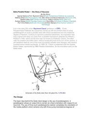
The goal of this project is to develop a <strong>ball</strong>-on-plate balancing system, capable of controlling the position of
a <strong>ball</strong> on a plate for both static positions and smooth paths. We intend that the initially horizontal plate
will be tilted along each of two horizontal axes in order to control the position of the <strong>ball</strong>. Each tilting axis
will be operated on by an electric motor. Each motor will be controlled using software, with a minimum of
position feedback for control. The position of the <strong>ball</strong> on the plate will be sensed through a resistive touch
screen.
The <strong>ball</strong>-on-plate system as implemented has limited consumer appeal. The challenge of balancing, however,
is a problem under continuous study for applications from robotics to transportation, often extensions of
the inverted pendulum project. Therefore, the system can present many challenges and opportunities as an
educational tool to university students studying control systems engineering.
The initial objective of the project is to maintain a static <strong>ball</strong> position on the plate, rejecting position
disturbances. An extension of this objective is movement to specified positions on the system: given a
position, a trajectory is plotted and the <strong>ball</strong> is moved to the new location. If this is extended further,
trajectories such as a circle or a figure-eight can be followed given judicious choices for <strong>ball</strong> position requests.
Characterizing system specs for such a system is difficult, notably because the desired motion is for an piece
of the system that is indirectly controlled. The controller cannot directly manipulate the <strong>ball</strong>, and therefore
deciding on the specs of the plate controller, in terms of rise time, settling time, and steady-state error is
difficult. With this in mind, the specifications of the overall system are < 2% error in the position of the
<strong>ball</strong>, with a settling time of less than 2 seconds, and for a nominal rotational speed (of the plate) of 1.35
rad/sec. This, in turn, mandates excellent response from the plate controller, including quick rise times,
rapid settling, and negligible steady-state error. Any error in the plate controller gets compounded into the
<strong>ball</strong> position, so overshoot, steady-state error and slow settling all present obstacles to ideal performance in
the <strong>ball</strong> positioning.
The project design plan is shown in Figure 1.1. As shown, the project needs to be broken into three subprojects:
the sensor system, the physical system, and the controller. These three projects will be developed
independently by the team, and then integrated into a complete system. The sensor subsystem consists of
the circuitry and software that generate coordinates from the touch screen. The physical system refers to
1

the design and machining of parts needed to construct the large yoke and axle, as well as the new motor
bracket, which are necessary to bear the weight of the touch screen. The control system includes not only
the modelling and simulation of the system as a whole, but additionally, the design of the controllers: one
for the <strong>ball</strong> position and another for the plate angles.
One of the major obstacles to integration and implementation is the reading of position coordinates from
the touch. A RS-232 serial card is supplied with the touch screen, however, the average position report rate
is 80-100 positions/second. Another obstacle is the system itself, which is open-loop unstable: the design
must take into account not only the dynamics of the two axis plate system, but also the dynamics of the
heavy steel <strong>ball</strong> moving around on the surface of the system.
2

Figure 1.1: Project Design Plan
3

Chapter 2
Professional and Societal
Consideration
As a product, the <strong>ball</strong>-on-plate system presents little in the way of a commercially viable product, except
perhaps as an exercise in control systems education. In that pursuit, however, there are still several prior
projects that tread the same path as this system, and thus patent protection would be difficult. Of immediate
similarity is the project created by the Professor Kevin Craig at Rensselaer Polytechnic Institute in the
Mechatronics program [4]. Ultimately, the differences between the project developed by Professor Craig’s
team and the project described in this report are implementational, with the ultimate objective of balancing
being the same. Professor Craig’s project however is inherently stable by design, whereas the project described
herein is naturally astable, therefore making the control somewhat more difficult. A second project
of similar scope was found upon search, created by Professors Graham Goodwin, Stefan Graebe and Mario
Salgado [5] from the University of Newcastle, Australia. The mechanism for balancing here is the same,
however, the feedback for <strong>ball</strong> position is generated using image processing techniques and a CCD camera
placed above the system. While investigating other projects, and additional search was made for patents
protecting designs or technology related to this system. This, however, yielded no systems related or similar
in operation to this project in the listings of protected inventions and designs.
If the project’s applications are taken to be academic and educational, considerations must still be made
with regard to the system’s safety and durability. Design decisions were therefore made that emphasized
the goal of a safe product that could be used for educational purposes. Wherever possible, metal edges were
filed and screw heads countersunk to prevent injury during a possible system instability. A polycarbonate
plate was placed across the rotational axis to protect the glass substrate of the touch screen, and to protect
the user should the touch pad become damaged. The glass in the touch screen is also chemically treated (i.e.
tempered), and while much stronger than untreated glass, also has the unique characteristic that instead
of forming sharp shards under fracture, it creates small, harmless bits of glass. With regard to software,
torque thresholds could be added to prevent violent behavior under unstable conditions. Another safety
measure is inherent to the operation of the touch screen coordinate system - should the <strong>ball</strong> break contact
with the plate, the system returns (0,0) positions. Should the <strong>ball</strong> leave the plate entirely, the system will
simply stay put. If desired, a further level of safety could even shut the system down upon retrieval of 0s to
4

the coordinate generator. Further development should also look into a more secure mounting system, since
simple metal C-clamps can loosen under repeated stress.
Should the system head into further revision, in preparation for manufacturing, several changes would have to
be made to make the system both commercially viable and capable of mass manufacture. Primary concern
rests on the inherent fallibility of the touch screen. Other touch sensitive technologies exist, albeit more
expensive, however it might be possible to source a supplier capable of building a resistive touch screen that
uses a polycarbonate or plastic substrate. This would cause a negligible change in cost, amortized over a
large production run, and would be a major boon to the overall product safety. Wire shielding is also of
major concern: the power wires running into the motors present a large, fluctuating electric field, which
tends to wreak havoc with the encoder wires, because the last 15 cm of wire are unshielded. This would be
a simple change resulting in a significantly better behaved system. Additionally, it might be recommended
to replace the secondary motor with a smaller, lighter unit, albeit with less torque. The secondary axis is a
light and balanced load, and requires significantly lower torques. This would in turn reduce the load on the
primary motor by reducing rotating mass, improving efficiency as well as safety.
5

Chapter 3
Design Procedure
3.1 Model development
In order to design a control system that will accurately control the position of the <strong>ball</strong>, a highly accurate
model of the entire system’s dynamics must be developed. As the accuracy of the model increases, the
uncertainty to be dealt with by the control effort will decrease. The model for our plate dynamics comes
from the general equation of motion for a multibody system,
M(θ) ¨ θ + B( ˙ θ) + C(θ, ˙ θ) ˙ θ + G(θ) = τ (3.1)
where M is the mass-inertia matrix of the system, B is the friction term, C is the velocity coupling matrix,
and G is the gravity loading vector. In most pan/tilt applications, there is no gravity loading on the first
joint. However, due to the altered orientation of our system (See Figure D.1), we have gravity loading terms
for both joints, as can be seen in Equation 3.2, the gravity loading vector for our system. Numeric values
for these terms can be found in Section 4.1.
−ma g sin(θ1)lca1 − ma g cos(θ1)lca2 − mb g sin(θ1) cos(θ2) lcb1 − mb g cos(θ1)lcb2 − mb g sin(θ1) sin(θ2) lcb3
G(θ) =
−mb g cos(θ1) sin(θ2) lcb1 + mb g cos(θ1) cos(θ2) lcb3
(3.2)
Unfortunately, using the linear control theory that we have learned thus far, it becomes difficult to develop
a control system for our fully nonlinear model. Because of this, the system must be linearized about a
trim condition in which the state derivatives are zero, i.e. ( ˙ θ, θ) = (0, θd). This operating point should be
specified in the angular region in which the system will spend the majority of its time, in our case θd = 0.
The linearization of the system can be derived as follows: The mass-inertia matrix can simply be evaluated
at θ = θd. Due to the trigonometric nonlinear terms in the gravity loading vector, we use a Taylor Series
expansion, keeping only the linear terms, and use the small angle assumption: sin(θ) ≈ θ and cos(θ) ≈ 1.
Since G is a function of both angles, f(θ1, θ2), we evaluate the gradient of G to determine the derivative terms
of the Taylor Series expansion with respect to both variables. The velocity coupling matrix C drops out
completely since all terms involve a θ 2 term. The friction term, B, is separated into its viscous and coulomb
6

components, and the coulomb terms are treated as an input disturbance. The result of this linearization is:
where Bu represents the control torque.
M(θd) ¨ θ + ∂G(θd)
(θ − θd) + Fv
∂θ
˙ θ = Bu − Fcsgn( ˙ θ) (3.3)
In order to facilitate the state-feedback control law u = −Kx (See Section 3.2), we must form the state-space
realization for this dynamic system. Defining our state vector as:
we can solve for our state variables:
x1 = θ − θd
x2 = ˙ θ
x1 ˙ = x2
x2 ˙ = M −1 (θd)
x :=
θ1 θ2 ˙ θ1 ˙
T θ2
Bu − Fcsgn( ˙ θ) − Fvx2 − ∂G(θd)
x1
∂θ
treating Bu as the control input, and Fcsgn( ˙ θ) as an input disturbance, the state-space form becomes:
⎡
⎢
˙x = ⎢
⎣
0 0 1 0
0 0 0 1
−M −1 (θd) ∂G
∂θ
2x2
−M −1 Fv
2x2
y =
⎤
1 0 0 0
0 1 0 0
⎡
⎥ ⎢
⎥ x + ⎢
⎦ ⎣
x
0 0
0 0
M −1 (θd) 0
0 M −1 (θd)
⎤
(3.4)
(3.5)
⎥
⎦ u (3.6)
With this linearized system, we can design a control law that will control the plate’s angular position based
on torque input. In addition to the plate dynamics, the <strong>ball</strong>’s response to plate position must be considered.
For our purposes, it should suffice to treat the <strong>ball</strong> and plate system as two decoupled <strong>ball</strong> on beam systems.
In addition, we will ignore any rolling friction that may occur between the <strong>ball</strong> and plate. This greatly
simplifies the model, and makes for easier control design. From the free body diagram in Figure 3.1, we can
obtain the dynamic equations that govern the <strong>ball</strong>’s motion [3]:
0 = ( J
+ m)¨x + mg sin(θ)
r2 ¨x =
mg sin(θ)
−
( J
r2 + m)
¨x = − mg
( J
r2 θ (3.7)
+ m)
7

Figure 3.1: Ball on Beam Free Body Diagram
Using the small angle approximation sin(θ) ≈ θ, we obtain Equation 3.7, where J is the <strong>ball</strong>’s inertia, r is
the <strong>ball</strong>’s radius, m is the <strong>ball</strong>’s mass, and g is the gravitational constant. Extended to two dimensions, the
state-space realization of the system becomes:
⎡
⎢
⎣
˙x
˙y
¨x
¨y
⎤
⎥
⎦ =
⎡
⎢
⎣
0 0 1 0
0 0 0 1
0 0 0 0
0 0 0 0
⎤ ⎡
⎥ ⎢
⎥ ⎢
⎦ ⎣
x
y
˙x
˙y
⎤
⎡
⎥
⎦ +
⎢
⎣
0 0
0 0
0
− mg
( J
r2 +m)
0 − mg
( J
r2 +m)
⎤
⎥ θ (3.8)
⎦
With these linearized equations of motion for the plate and <strong>ball</strong>, we can begin to design our controller.
3.2 Control development
To control the Ball on Plate Balancing System, we have decided to employ a full state-feedback controller.
Though classical control design approaches may have been sufficient, we felt as though we would achieve
better results with state-feedback. One reason that state-feedback control is particularly advantageous is
that all information regarding oscillatory modes and initial conditions is available, which is not the case
with classical frequency domain methodologies [6]. The state-feedback control will also utilize an observer
to estimate the velocity states of the system. This will be mentioned in more detail later in this section.
Before developing the controller and observer, we must first check to see that the system is both controllable
and observable, i.e. we can influence all system states through our control input, and that they will be visible
at the output. To verify this, we must ensure that the Controllability and Observability matrices are full
rank:
C = B AB A 2 B . . . A n−1 B
O = C CA CA 2
. . . CA n−1 T
For our linearized systems as given in Equations 3.6 and 3.8, they are both fully controllable and observable,
so we may continue on to the control design phase.
For plate control, we use a Linear Quadratic Regulator (LQR). This serves to find the optimal control input,
u(t) that will drive the system from it’s initial states, x(t0) to some final value, x(tf ), while minimizing a
(quadratic) cost function:
tf
J =
0
x T Qx + u T Rudt (3.9)
8

where Q is the state penalty matrix, and R is the control penalty matrix [7]. These are user defined matrices,
whose proper selection will achieve the desired time-domain response. The optimal feedback gain matrix,
K can be found using K = R −1 B T P where P is is a positive definite solution to the Steady State Riccati
Equation:
PBR −1 B T P = PA + A T P + Q (3.10)
Once the feedback gain matrix has been found, we can form the control law
u = −Kx (3.11)
that will drive our the system states to the desired values. This, however, assumes that we can measure all
four of the states as defined in the state vector in Equation 3.4. In reality, we can only directly measure x1
and x2, the angular position of the plate, and not the velocity. For this reason, we develop a state observer
that will estimate the values of x3 and x4. This is done by creating a copy of the linear dynamic equations,
and adding an output term:
˙ˆx = Aˆx(k) + Bu(k) + L(y(k) − ˆy(k)) (3.12)
ˆy(k) = Cˆx(k)
where ˆx is the observer’s estimate of the system states, u is the system input, y is the plant output, and
ˆy is the observer output. The L matrix ensures that the observer error, ˆx(k) − x(k) converges to zero [2].
Much like LQR was used to determine the optimal feedback gain matrix, K, we will use a Kalman filter
to determine the optimal observer gain matrix, L. Normally, a Kalman filter bases its calculation on the
covariance matrices of the process and measurement noise. However, for simplification, we will use a more
heuristic approach, much like deciding the values for the Q and R matrices for the LQR control. More detail
on this can be found in Section 4.2. Once the observer gain matrix has been found, we can easily implement
the control in (discrete) state-space form:
ˆx(k + 1) = (A − BK − LC)ˆx(k) + Ly(k) (3.13)
u(k) = −Kˆx(k)
where the output of the observer becomes u(k), the control torque , and the output of the plant, i.e. encoder
feedback, is the input to the observer.
The same procedure is followed to develop a controller for the <strong>ball</strong> dynamics. However, instead of using
LQR to determine the feedback gain matrix, K, we simply use pole placement, the mathematics of which
we will forego discussing in detail in this report. See [8] for a discussion of pole placement, as well as a more
detailed discussion of state-feedback control and LQR in general. LQR is used to determine the observer
gains. Details on this can be found in Section 4.2.
3.3 Physical design
Several physical components in addition to the motors, shafts, gears, belts, and encoders were necessary in
order to realize the construction of the system. These custom made parts included a specialized axle, yoke,
and motor mounting bracket. Each of these parts of the system were machined out of aluminum stock and
their full dimensions are included in Appendix D. Specific attributes of the system of course required the
parts to have certain features. The lengths and widths of the yoke were designed to fit the size and shape of
9

the touch screen that was used in the project with some slight clearance along the long side of the yoke to
allow for wiring to move freely.
The special axle was designed to support the touch screen on the tilt axis. It was formed of several pieces
to allow for set screw adjustment of the height. This allowed for materials of varying thickness to be placed
on the axle while keeping the actual plane of the touch screen coincident with the axes of rotation. In the
final design these materials included a polycarbonate plate, the touch screen itself, and a rubber membrane
to provide friction that will force the <strong>ball</strong> to roll instead of slide.
Finally the motor mount bracket was created to fix the tilt axis motor to the system. It was designed to
place the motor directly behind the yoke to reduce the inertia effects of the heavy motor as much as possible.
3.4 Touch screen subsystem development
Ball position feedback is accomplished through the usage of an analog resistive touch screen element. Screens
of this type are often used in public information kiosks and cashier stations, allowing the user to interact
with the screen directly. As the feedback in this system, the touch screen will read the application of pressure
by a steel <strong>ball</strong> and track it as it moves within the active portion of the screen.
An analog resistive touch screen works using a simple design. Two layers of material are coated with indium
tin oxide (ITO) to give them a known resistance, something between 100 and 500 Ω/sq. depending on the
manufacturer and the application. The two layers are then placed 90 ◦ offset from each other on top of a glass
or polycarbonate substrate, with a grid of transparent insulating dots separating the layers. Silver bus bars
are placed at the edges to allow the application of voltage across the layers. To generate a touch position, the
user or an object must exceed the activation force of the screen, pressing the two layers together. This creates
an electrical connection between the layers. However, both X and Y axes cannot be read simultaneously,
because the concept works by applying a voltage across one layer, and looking for the voltage that appears
on the other layer. Therefore, the system works by alternately applying a voltage to one layer and reading
off of the other. The voltages are then read in by an analog-to-digital (A/D) converter to be used as a
coordinate value[1].
There are, however, several types of analog resistive touch screens, notably 4-wire, 5-wire and 8-wire. These
designations refer to the number of wires between the screen and the screen controller. 4-wire screens operate
by applying voltage across the two wires for one layer, and reading a voltage from the ground wire of the other
layer. The voltage application and read operation then swaps around for the other layer. The 5-wire screens
use the bottom layer for both axes measurements, applying voltage across the top layer only. This simplifies
measurement and voltage application duties over the 4-wire screen. The 8-wire screen is an extension of the
4-wire screen, using the additional 2-wires per layer to provide a stable voltage gradient. This makes the
8-wire screen immune to voltage and resistance fluctuations due to ambient heat and humidity or aging of
the screen. The pin configuration for an 8-wire screen is shown in Table 3.1[1].
Table 3.1: Touch screen pin-out
Axis Xe + Xe − Y e + Y e − Xs + Xs − Y s + Y s −
X 5v GND NC READ Ref+ Ref- NC NC
Y NC READ 5v GND NC NC Ref+ Ref-
10

Due to pricing and immediate availability, an 8-wire screen was selected for this project. The advantages
of the 8-wire over the 4-wire screen aren’t really relevant to this project, however the stability of the 8-wire
screen certainly helps during testing. The difficulty with the 8-wire screen, however, is the requirement
for ratiometric A/D converters. Ratiometric A/D converters use the applied voltage at the location being
converted as the reference for the conversion, instead of a using a static reference. This accounts for variations
in the supply voltage, as well as variations in the transmission lines caused by noise or interference. Originally,
it was planned that the A/D conversion for the touch screen would be done by the ARCS system, using
full 16-bit resolution and a 1 ms sampling period. The ARCS board A/D converters are unfortunately not
ratiometric. Further complicating things was a significant difficulty in generating position coordinates using
a regulated power supply and an oscilloscope. The choice was therefore made to use the RS-232 touch screen
controller included with touch screen purchase. Using 10-bits of resolution enables the controller to have
a maximum theoretical 1024x1024 positions on the surface of the touch screen. This, however, is limited
to a subset of the full range, (100-900)x(100-900) positions, due to losses in drive voltage from the various
transmission lines leading to the screen itself. The layout of the voltage ranges with the corresponding digital
values is shown in Figure 3.2[1].
Figure 3.2: Touch screen A/D conversion layout
Using the serial touch screen controller with MATLAB and xPC Target requires using the RS-232 blocks
available in the xPC Target Simulink block library. During regular operation, the controller sends data
11

egardless of any receiving device. Therfore, MATLAB merely has to process the data as it comes in,
convert the digital values to real-world coordinates, and then pass them along to the <strong>ball</strong> controller. This is
discussed further in Section 4.4.
The analog resistive touch screen was chosen as the <strong>ball</strong> feedback for this project for several reasons. The
primary reason is simplicity, both of the sensing operation and the circuitry/software required to generate
coordinates. This is even further enhanced by the availability of simple serial controller cards and chips which
can generate position coordinates without any configuration or setup. Certainly, if one were so inclined, a
video processing system could be constructed that is capable of generating similar results. However, a system
of this type of equal ability to the touch screen is limited by a number of things:
1. A CCD capable of generating frame rates fast enough to match what a simple touch screen controller
is capable of would be prohibitively expensive (≥ 100 frames/sec)
2. The video from the CCD needs to be handed off to a frame-grabber capable of reading video at the
same frame rate (≥ 100 frames/sec) which is prohibitively expensive
3. MATLAB xPC Target is very limited in the ways in which it can receive data, as it doesn’t really have
a vast driver set, and therefore any frame grabber card would need a custom driver in order to pass
video frames to MATLAB
4. Once the video is brought into MATLAB, further processing still needs to be done to process the image
and find the centroid of the <strong>ball</strong>
5. The position coordinate processing algorithm would need to be sufficiently robust to deal with varying
brightness and reflections and noise in the video signal
This list isn’t to suggest that a video processing system isn’t possible with a <strong>ball</strong>-on-plate system, merely
that with the resources available for this college design course, a touch screen made the most sense.
Other touch sensitive technologies exist outside of the basic analog resistive system. These include infrared,
capacitive, near field imaging (NFI), and surface acoustic wave (SAW). Each has advantages that make it
better for certain applications. However, in trying to track a <strong>ball</strong>, capacitive sensing requires the electrical
activity of a human hand. Infrared is also not as accurate as the other technologies and is sensitive to
variations in ambient light. Of those technologies remaining, NFI, SAW and resistive, resistive touch screens
are by far the least expensive to acquire and implement, and are very durable. This made the resistive touch
screen the ideal choice for this application, due to budget constraints.
12

Chapter 4
Design Details
4.1 Modeling
To determine numerical values for the state-space representation of the system dynamics as derived in
Section 3.1, we must first identify the unknown parameters of the system, i.e. inertia and friction. To
identify the inertia of the system, a Solidworks model of the system was made. The inertia of each link
about its center of mass with respect to our defined coordinate systems (as shown in Figures D.2 and D.3)
was determined by Solidworks. The values for the inertia tensors are shown in Equation 4.1. It should be
noted that the inertia tensor of link B, Jb, only contains diagonal values, whereas Ja does not. This is due
to the fact that Body B has uniform mass, and Body A does not due to the offset mounting of the motor as
seen in Figure D.1
⎡
Ja = ⎣
.0277 −.0001 −.0003
−.0001 .0209 .0065
−.0003 .0065 .0070
⎤
⎡
⎦ Jb = ⎣
.0045 0 0
0 .0010 0
0 0 .0035
⎤
⎦ (4.1)
Identification of the friction in the system was performed as follows: A Simulink model capable of measuring
the encoder and outputting constant voltages was used in conjunction with a MATLAB script to repeatedly
estimate the velocity of each joint. For each of 200 voltage increments from minus two volts to plus to
volts, the motor was allowed to turn for ten seconds so that it would reach steady state velocity. The
last four seconds were then averaged to obtain a single value for steady state velocity for that particular
torque (voltage). In addition, a one second ten volt spike was added in the beginning of each run in order
to overcome the stiction of the system. By plotting this data and finding a least squares approximation
for the data, the coulomb and viscous friction were found as the intercept and slope of the regression line,
respectively. The plots for each axis are shown in Figures A.1 and A.2.
With these parameters identified, we can substitute numerical values into Equation 3.6 and begin to design
our controller. However, since we have fully identified the system model, we can use feedback linearization
to, in effect, cancel out the gravity and viscous friction terms. This will be discussed further in Section 4.2.
13

Assuming that gravity and friction can be perfectly cancelled, we can obtain the linear state-space model
either from Equation 3.6, or using MATLAB’s linmod() function. The resulting state-space is shown in
Equation 4.2.
˙x =
⎡
⎢
⎣
0 0 1 0
0 0 0 1
0 0 0 0
0 0 0 0
⎤
⎡
⎥ ⎢
⎥
⎦ x + ⎢
⎣
0 0
0 0
66.73 0
0 100.8037
⎤
⎥
⎦ u (4.2)
Equation 4.2 shows the linear dynamic equations that are used to develop the control system.
For the <strong>ball</strong> dynamics, all values in Equation 3.8 are known constants. The inertia of the <strong>ball</strong>, J, can be
found from the equation for the inertia of a sphere [9]:
Substituting in the following values:
J = 2
5 mr2
m = .13kg
g = 9.81m/sec 2
r = .0158m (4.3)
we obtain the final state-space representation of the <strong>ball</strong> dynamics, as shown in Equation 4.4.
⎡ ⎤
˙x
⎢ ˙y ⎥
⎣ ¨x ⎦
¨y
=
⎡
0
⎢ 0
⎣ 0
0
0
0
1
0
0
⎤ ⎡ ⎤
0 x
1 ⎥ ⎢
⎥ ⎢ y ⎥
0 ⎦ ⎣ ˙x ⎦
0 0 0 0 ˙y
+
⎡
0
⎢ 0
⎣ −7
0
0
0
⎤
⎥
⎦ θ (4.4)
0 −7
4.2 Control
The control scheme for the Ball on Plate Balancing System consists of two loops: an inner loop to control
the motor torque based on a desired plate angle, and an outer loop to command a plate angle based on a
desired <strong>ball</strong> location. In order to successfully implement this design, the inner loop must have a much faster
response than the outer loop. Since the inner loop can only be designed to be as fast as physical limitations
allow (motor torque, etc.), we must intentionally design the outer loop to be slower.
As mentioned in Section 3.2, we decided upon the use of a Linear Quadratic Regulator for the purposes
of plate positioning. Successful implementation of this depends on our defined state and control penalty
matrices, Q and R. Since we want to accurately track the angular position of the <strong>ball</strong>, and care less about
the angular velocity, we choose the Q matrix to have a high weighting on the position states. Adjustment
of the R matrix will either promote or penalize the control effort. By altering these values, we can further
adjust the time-domain response, while making sure not to operate in the saturation region of our motors.
For this reason, it is important to take the motor saturation into account when designing the simulation.
14

The final values of Q and R are shown in Equation 4.5.
⎡
1000
⎢
Q = ⎢ 0
⎣ 0
0
1000
0
0
0
1
⎤
0
0 ⎥
0 ⎦
0 0 0 1
R =
.5 0
0 .5
With these state penalty matrices, the state gain matrix was calculated with MATLAB, and is shown in
Equation 4.6.
44.7214
K =
0
0
44.7214
1.8277
.0001
.0001
1.6992
(4.6)
This places the closed loop eigenvalues at:
(A − BK) = [−88.0, −138.8, −33.8, −32.5] T
When designing an observer to estimate the system states, it is important to make the observer’s dynamics
much faster than that of the closed-loop system. As mentioned in Section 3.2, we used a Kalman filter to
calculate the optimal observer gain matrix, L. Just as with the LQR design for the controller, the Q and R
matrices we chosen to give the best results. The optimal solution would be derived using the process and
sensor noise covariances, however we simply use the matrices as ”weights” as we did with LQR. The final
values for these matrices are seen in Equation 4.8.
Q =
resulting in the observer gain matrix:
100000 0
0 100000
L =
which places the system’s closed-loop eigenvalues at:
⎡
⎢
⎣
R =
205.4 −.0438
−.0438 252.5
21101 −10.03
−10.03 31876
.01 0
0 .01
⎤
⎥
⎦
(A − BK − LC) = [−211 ± j186, −163 ± j149] T
(4.5)
(4.7)
(4.8)
(4.9)
(4.10)
Normally, the observer eigenvalues should be roughly 5-10 times faster than the closed-loop eigenvalues.
In our case, they are not quite that fast, however the observer estimates the system states very well, and
increasing the speed of the observer’s dynamics yields negligible differences. Figure 4.1 shows how well the
observer tracks the system states for a step response, and Figure 4.2 shows the observer error as a function
of time. It should be noted that these responses were generated using the nonlinear plate dynamics.
Bode plots showing the open-loop frequency response of the inner-loop are shown in Figures A.3 and A.4.
Gain and phase margins for both the inner-loop and outer-loop are summarized in Table 4.1.
A similar design procedure is used to develop the outer-loop controller for the <strong>ball</strong> dynamics in Equation 4.4.
Instead of LQR, we use pole placement to move the closed-loop eigenvalues to the desired locations. For our
case, we chose to place all closed-loop poles at s = −1.25 ± j1.5. This corresponds to a natural frequency of
15

Figure 4.1: Observer State Estimation - Plate
Figure 4.2: Observer Error - Plate
16

wn = 1.95 and a damping ratio of ζ = .64. Using MATLAB’s place() command, we compute the feedback
gain matrix to be:
−.5446
K =
0
0
−.5446
−.3571
0
0
−.3571
(4.11)
After several design iterations, we find the Q and R matrices to be:
⎡
100000
⎢
Q = ⎢ 0
⎣ 0
0
100000
0
0
0
1
⎤
0
0 ⎥
0 ⎦
.01
R =
0
0
.01
0 0 0 1
resulting in the observer gain matrix:
L =
⎡
⎢
⎣
3162.3 0
0 3162.3
10 0
0 10
The open-loop frequency response for the outer-loop is shown in Figure A.7.
Table 4.1: Gain and Phase Margins
Gain Phase
Pan ∞ -147 deg at 38.4 rad/sec
Tilt -187 dB at 0 rad/sec -147 deg at 47.2 rad/sec
Ball 70 dB at 112 rad/sec 76.1 deg at 0.974 rad/sec
⎤
⎥
⎦
(4.12)
(4.13)
Figure A.5 shows how well the observer tracks the system states, and Figure A.6 shows the observer error
as a function of time. It can be seen in the figures that the observer is able to estimate the system states
with almost no error. Note that the vertical scale in both Figures 4.2 and A.6 is on the order of 10 −3 .
4.3 Simulation
When any engineering problem is approached, it is desirable, if not absolutely necessary that a simulation of
the system is made. This allows the engineer to analyze and test their design before actual implementation.
The need for this becomes obvious if one considers very large, expensive systems such as an aircraft. One
would obviously not want to build an aircraft, and then fly it to see if the flight controls work. It is important
to remember that the validity of a simulation depends greatly on the accuracy of the model. For this reason,
we developed a simulation around the full nonlinear model of our Ball on Plate system. The simulation
takes into account nonlinearities such as gravity loading, coulomb and viscous friction, torque saturation,
encoder quantization, touch screen quantization, and the multiple sampling rates of our system. Figure 4.3
shows a Simulink block diagram that represents the entire Ball on Plate Balancing System. This section will
discuss the function and purpose of each block. The trajectory generation block serves command the desired
<strong>ball</strong> position. This may take on the form of a specific coordinate, or some path such as a sinusoid. The
control/observer blocks are the state-space implementations of the state-feedback controller, u = −Kx, and
17

Figure 4.3: Simulink Block Diagram
the observer estimate, ˆx. The gravity and friction linearization blocks simulate the feedback linearization
that we are employing to negate the nonlinear gravity and friction terms of the system. They are then added
to the control torque (output from the plate controller), and passed onto the nonlinear plate dynamics block.
This block is the heart of the simulation, and takes into account all of the aforementioned nonlinearities.
In the actual implementation, this block is replaced by the amplifier block. The output of this block (plate
angle) is fed into the linear <strong>ball</strong> dynamics block. In reality, this block would be replaced by the encoders.
The output of the <strong>ball</strong> dynamics is fed into a touch screen simulation. This block takes into account the
quantization and sampling rate of the touch screen. The interpolation filter, as described in Section 4.4, is
also included in the simulation.
Various plate and <strong>ball</strong> control tests were run with the simulation before the actual control implementation.
The first test was the tracking ability of plate control (a step response can be seen back in Figure 4.1).
Figures A.8 and 4.4 show the results for tracking a sinusoid at 3 rad/sec. The closeup shows the slight
error at low velocity. This error becomes magnified in the actual implementation due to friction. The next
simulations were a step response and sinusoid tracking for the <strong>ball</strong> position. Figures A.9 and 4.5 show the
results of this. The sinusoid tracking shows a very large phase delay. This stems from the fact that the
outer-loop must be slow to allow the plate to position itself properly. Unfortunately, this speed difference
causes a large phase delay. However, despite the delay, the <strong>ball</strong> tracks the amplitude of the sinusoid very
well. Both responses were for a desired amplitude of 0.05 m, which is roughly half the distance of the plate,
and 1 rad/sec. Additionally, a circular <strong>ball</strong> trajectory was commanded. The results of this are shown in
Figure A.10.
To better visualize the simulation results, a 3D animation was generated using MATLAB’s Virtual Reality
Toolbox. Here, we will briefly describe the steps taken to create this animation. The reader is encouraged to
refer to the Virtual Reality Toolbox documentation for more detailed information. The first step in creating
the animation was to export the Solidworks model as a VRML97 file. Solidworks exports a single *.vrml
file, which contains a model for each part as defined in Solidworks. Using the V-Realm Builder by Ligos
Corp. (included with the virtual reality toolbox), we can group specific parts to form the bodies, as defined
18

Figure 4.4: Plate Sinusoid Tracking - Closeup
Figure 4.5: Ball Position Sinusoid Tracking - 1 rad/sec
19

in Figures D.2 and D.3. A group for Body B was created as a sub-group within Body A, and the <strong>ball</strong> was
placed in a sub-group within Body B. Then, in each of these groups, the rotational axes were defined. These
are the axes which the virtual reality toolbox will use to control the movement of the objects. Using this new
VRML97 file, we can create a Simulink block diagram to control the animation. A VR Sink block is placed
in the Simulink diagram, and the *.vrml file we created previously is loaded into this file. In the VRML tree
pane in the properties of the VR Sink block, we enable the checkboxes that correspond to the rotational
axes that we defined using V-Realm Builder. Rotation nodes were selected for the two main bodies, and a
translation node was used for the <strong>ball</strong>. Figure A.15 shows the block parameters window for the VR Sink
block. The ”view” button in the block parameters window initializes the animation, and shows the object.
Finally, data from a previously run simulation, which is stored to the workspace, is fed into the VR Sink
block, as shown in Figure A.16. Once the Simulink simulation is run, the animation begins. This animation
is able to replicate any results from the simulation. Figure A.17 shows the output window.
4.4 Touch screen subsystem
The touch screen interface to MATLAB relies entirely on the capabilities of the 3M Dynapro SC3 serial
interface controller for its operation. Every touch controller ”report” consists of an X-Y coordinate pair.
The SC3 controller takes these X-Y coordinate pairs it generates and converts them into sets of three 8-bit
packets which can be converted into coordinate pairs. The actual coordinate values are 10-bit values, that
are actually spread across the three separate packets as shown in Table 4.2. Note that in the table, the P
bit refers to the status of the ’pen’, or the object touching the pad: 1 is pen down, 0 is pen up. Also note
that x9 refers to the 10th bit of the 10-bit x coordinate number, and so forth for all xk and yk[1].
Table 4.2: Touch screen controller packet composition
Packet/Bit # 7 6 5 4 3 2 1 0
#1 (sync) 1 P x9 x8 x7 y9 y8 y7
#2 (data) 0 x6 x5 x4 x3 x2 x1 x0
#3 (data) 0 y6 y5 y4 y3 y2 y1 y0
All of these packets are sent asynchronously and without prompting: as soon as the touch screen receives
sufficient pressure for the controller to register a touch, the system begins to send data. In order to process
this data, and get the resultant coordinate information into the real-time computer, a serial interface needs
to be created in MATLAB Simulink that can be compiled for the xPC Target system.
The basic overall system utilizes the binary receive block in Simulink to retrieve data as sets of three 1-byte
packets as described in the manual. The RS232 Setup block sets the link parameters as 2400 bps, and 8-N-1 -
8 bits per packet, no parity, and 1 stop bit. Normally, Simulink is unable to utilize binary numbers, however,
the Communications Toolbox allows conversion to and from binary. This makes possible the individual bit
manipulation necessary to move the 8-bit packets from the controller into the 10-bit binary words that the
controller’s A/D converter creates. The Simulink diagrams for this system can be seen in Figures 4.6 and
4.7.
After assembling the Simulink system and using the steel <strong>ball</strong> to generate coordinate paths, it becomes
obvious that while the touch screen does generate a great many points, it generates a number of coordinates
20

Figure 4.6: Simulink touch screen interface
Figure 4.7: Simulink touch screen packet conversion
21

in the same area due to settling time settings in the controller. The result is the series of steps shown in
Figure 4.9. If integrated with the <strong>ball</strong> controller and the plate controller, this stepping would result in very
abrupt movement and poor performance.
After several unsuccessful attempts to send the controller configuration commands, it was decided that the
easiest alternative was to pass the generated coordinates through a low-pass filter. The abrupt changes in the
output coordinates are equivalent to a step command, so in order to smooth it, a simple first order low-pass
filter was created, with a cutoff at 50 radian/second. This cutoff was chosen to maximize data retention,
namely small fluctuations in output, but to remove the large jumps in output that would cause problems
with the controllers. The transfer function, in continuous time, is
Fc =
1
1 + s
50
(4.14)
If this is converted to discrete time, using the controller’s sampling period of 1 ms with a zero-order hold,
the transfer function is
Fd = 0.04877
z − 0.9512
(4.15)
The bode plot of this filter is shown in Figure 4.8. The -3db point of the now discrete filter is around 50
radians/sec as designed, with a decent roll-off, though that isn’t terribly important. The objective is to
reduce the amplitude of much higher frequencies, which this filter does as shown in Figure 4.9, looking at
the now much smoother sine wave.
Figure 4.8: Touch screen filter - Bode plot
With the coordinates smoothed, the remaining work is to scale and map the coordinates. First of all, the
coordinates generated by the touch screen are based on a reference point of (0,0) in the top left corner, as
seen in Figure 3.2. The controller, however, assumes (0,0) to be the center of touch screen, which is really
22

Figure 4.9: Touch screen output filtering
Figure 4.10: Touch screen output filtering (close-up)
23

coordinate point (512,512). To map the coordinates to this new space, each generated coordinate is reduced
by 512 to find the new coordinate. The controller is also expecting displacements from the center (0,0) point
in meters. To scale the coordinates to meters, the known resolution and size of the touch screen is utilized
to find the meters per digital level generated by the touch screen controller.
.12065 m
512 levels = 2.356 × 104 meters/level (X)
.09525 m
512 levels = 1.860 × 104 meters/level (Y )
24

Chapter 5
Design Verification
Several steps were taken to verify the design of both the individual components of the <strong>ball</strong> on plate system,
as well as the system as a whole. These included comparison of simulated and experimental results of: the
effects on the inactive system due to a sudden release from an unstable point, step responses, sine wave
tracking, and a friction and gravity cancellation experiment. The touch screen design was also verified
through several experiments, and finally the overall performance of the system was rigorously tested as the
controller was tuned for the best results. Videos are available upon request and included with the electronic
version of this report.
In the first experiment, the system was set up with the motors disabled but the encoders active. The system
was then rotated by hand and raised up to the level position at which the system will operate. Dropping
the system and allowing gravity to do its work, the response on the pan axis was recorded by the encoder.
This same scenario was then developed in simulation, and the plots of position versus time for each were
compared.
Shown in Figure 5.1 are the resulting plots for both the actual and simulated responses. The graph demonstrates
that there is a close match including the rise times, settling times, and shape of the response.
A step response for a 0.5 rad position command and then a 2 rad/sec sine wave input were also applied to
the system both in in the actual physical system. The plots for each are shown in Figures 5.2 and 5.3.
By examining the plots, the step responses of the simulated and experimental form a close match. In
addition, sine wave tracking matches nearly perfectly. With the exception of a slight flattening at the top of
the experimental resulting sine wave, the desired, simulated, and experimental are all identical.
In order to further verify the design, a friction and gravity cancellation experiment was devised. By inputting
only the friction and gravity terms that are used for feedback linearization in the system, it was possible to
observe the effects of the cancellation on the physical system. When the experiment was running, the once
heavy and unbalanced physical system could be moved to any position by hand with ease and this position
was held in place. In addition, a light push on the system resulted in the system spinning about the pan
axis six to eight times due to the reduced friction. Figure A.18 shows a plot of the exactly constant torque
output for the system at its balancing position is shown. The torque output value was 0.38 N-m. This value
matched both simulation as well as hand-written calculations for the amount of torque necessary to hold
25

Figure 5.1: Model validation - drop
Figure 5.2: Step response - 0.5 radians
26

Figure 5.3: Sine wave tracking - 2 radians/sec
up the heavy system. A video demonstration is available upon request and included with the multimedia
version of this report.
As discussed earlier, the touch screen interface was designed through and xPC Target serial interface to
the touch screen controller card. Upon completion of the design various tests were performed to view the
subsystems ability with tracking the <strong>ball</strong>. Figures A.19 and A.20 are plots of several inputs traced on the
touch screen by actually rolling the <strong>ball</strong>. The first is simply a square with diagonals drawn across it. The
second is a more complicated rendition of the name ”Chris” in cursive handwriting. Both showed very good
results.
Final design verification of course occurred during the testing and tuning of the final system. Through
rigorous testing, sometimes complicated by touch screen malfunction, the various objectives of the project
for static balancing and path following by the <strong>ball</strong> were observed. After some tuning, <strong>ball</strong> balancing for a
static position worked well. Given a commanded location of the origin (center of the plate), the system was
capable of correcting even extreme disturbances to the <strong>ball</strong> location within a minimal amount of time and
oscillations about the desired point. Steady state error was also at a minimum. In addition, path following
along a straight line worked well to a degree, though there was some oscillation about the line as the <strong>ball</strong>
rolled along its path. For a circle trajectory, the best result for the <strong>ball</strong>s path was more of an oval shape.
Demonstration videos qualitatively well demonstrate the results of the design, however touch screen failure
immediately following these good results has prevented any collection of quantitative verification data such
as desired versus actual <strong>ball</strong> position information for static positions. This is unfortunate; however it is
extremely fortunate that such excellent video was captured before the failure of the touch screen. Upon
replacement, further data could be collected.
A simple tolerance analysis test to verify the gain and phase margins (qualitatively) is to give the system a
27

disturbance while in operation. While the system was being commanded to follow a sine wave input, we held
the yoke from moving by hand. After letting go, the system sped up to catch up with the desired trajectory,
and then fell back into sync.
28

Chapter 6
Costs
Table 6.1: List of parts
Item Qty Cost Total Source
1 1/4” diam. 440C stainless <strong>ball</strong> 1 $9.17 $9.17 McMaster-Carr
3M Dynapro 95640 10.4” 8-wire resistive touch screen 1 $39.00 $39.00 Ebay
3M Dynapro SC3 4/8-wire resitive touch screen controller 1 Ebay
Pittman motor GM9234S017 (pan) 1 $97.59 $97.59 Supplied
Pittman motor GM9234S017 (tilt) 1 $97.59 $97.59 Supplied
Pan gear A 1 $9.97 $9.97 Supplied
Pan gear B 1 $22.02 $22.02 Supplied
Tilt gear A 1 $7.95 $7.95 Supplied
Tilt gear B 1 $22.02 $22.02 Supplied
Pan belt 1 $3.92 $3.92 Supplied
Tilt belt 1 $3.55 $3.55 www.sdp-si.com
Misc screws $5.00 $5.00 Home Depot
Total $269.61
Table 6.2: List of raw materials
Item Qty Cost Total Source
1/2” aluminum stock 5 lb $4/lb $20.00 RPI Machine Shop
1/16” latex rubber membrane 1 $9.38 - 12”x12” $9.38 McMaster-Carr
.093” Lexan panel 1 $5.00 - 8”x10” $5.00 Home Depot
Total $34.38
29

Table 6.3: Labor costs
Description Hours Cost Total
Andrews, Greg [Engineer] 300 $35/hr $10,500
Colasuonno, Chris [Engineer] 300 $35/hr $10,500
Herrmann, Aaron [Engineer] 300 $35/hr $10,500
Caskey, Ryan [Machinist] 30 $35/hr $1,050
Total 930 $32,550
30

Chapter 7
Conclusions
In conclusion, overall the system can be considered a success. The objective of the project was to control the
position of the <strong>ball</strong> on the plate for static positions and smooth paths, as well as have the system capable
of correcting for disturbances in <strong>ball</strong> position. In general these goals were accomplished, especially static
position balancing and disturbance rejection. The <strong>ball</strong> can be centered on the plate or another coordinate
location, and will quickly correct for even large disturbances to the <strong>ball</strong> position with fast response time,
small overshoot, and a very minimal steady state error. Comparing to the original design specification, the
<strong>ball</strong> is returned to its location with approximately 2% error, however due to touch screen failure, we do
not have quantitative data to support this. The settling time is slightly longer than 2 seconds; however in
hindsight this may have been extremely fast target for settling a large disturbance. Additionally, the plate
is able to track well beyond 1.35 rad/sec. From an observers point of view the system definitely responds
well.
As for path following, the more advanced possible objective for this system, there was also a good deal
of success. For simple straight line paths, (especially moving along the tilt axis) the system performed
moderately well, though there were some slight oscillations about the intended path. It is believed that this
could be improved through some improvements to the design of the system.
One apparent issue is related to the system’s friction cancellation. With imperfect friction cancellation, there
is a possibility that the controller will request a very small torque from the motors but that this request
will be less than the remaining friction in the system. Thus, the motor will not actually make this response.
This possibility could explain some of the oscillation that occurs during path following. If the friction of the
system can more accurately be modelled, perhaps the overall performance of the system could be improved.
Lastly, another option would be to recreate the system using nonlinear control methods. This may or may
not make an improvement but it would be interesting to examine.
With more time, it would also benefit the system to revise the touch screen interface. The simplicity of
using the touch screen controller card and the time limitations of the project lead to the use of the serial
communication method. Using the serial connection and touch screen controller card resulted in a limitation
of the touch screen resolution of approximately 1024x1024. By devising an interface that uses A/D converters
directly on the touch screen output, a much higher resolution could be achieved thus reducing error in the
known <strong>ball</strong> position.
31

Bibliography
[1] 3M Touch Systems. SC3 Touch Screen Controller: User’s Guide, 2nd edition, 2003.
[2] Dr. Murat Arcak. Discrete time systems - lecture notes. 2003.
[3] No Author Available. Control tutorials for matlab: Modeling the <strong>ball</strong> and beam experiment. Available
WWW: http://wolfman.eos.uoguelph.ca/ ∼ jzelek/matlab/ctms/examples/<strong>ball</strong>/<strong>ball</strong>.htm.
[4] S. Awtar, C. Bernard, N. Boklund, A. Master, D. Ueda, and K. Craig. Mechatronic design of a <strong>ball</strong>-onplate
balancing system. Technical report, Rensselaer Polytechnic Institute, 2002.
[5] Graham Goodwin, Stefan Graebe, and Mario Salgado. Control system design - <strong>ball</strong>-on-plate tutorial.
Available WWW: http://csd.newcastle.edu.au/control/simulations/<strong>ball</strong> sim.html, 2001.
[6] Dr. Russell Kraft. Computer applications lab - hybrid control. 2004.
[7] Dr. Russell Kraft. Computer applications lab - optimal control. 2004.
[8] C. Phillips and H. Nagle. Digital control system analysis and design, third edition. Technical report,
Prentice Hall, Inc., 1995.
[9] Eric W. Weisstein. Moment of inertia - sphere. Available WWW: http://scienceworld.wolfram.com/
physics/MomentofInertiaSphere.html.
32

Appendix A
Diagrams and Figures
Figure A.1: Pan Axis Friction Data
33

Figure A.2: Tilt Axis Friction Data
Figure A.3: Frequency Response - Pan Axis
34

Figure A.4: Frequency Response - Tilt Axis
Figure A.5: Observer State Estimation - Ball
35

Figure A.6: Observer Error - Ball
Figure A.7: Frequency Response - Outer-loop
36

Figure A.8: Plate Sinusoid Tracking - 3 rad/sec
Figure A.9: Ball Position Step Response
37

Figure A.10: Ball Circular Trajectory
38

Figure A.11: Nonlinear plate dynamics block diagram
Figure A.12: Linear <strong>ball</strong> dynamics block diagram
39

Figure A.13: Gravity compensation block diagram
Figure A.14: Friction compensation block diagram
40

Figure A.15: VR Sink Parameters Window
Figure A.16: Virtual Reality Simulation Block Diagram
41

Figure A.17: Virtual Reality Animation Window
Figure A.18: Gravity cancellation
42

Figure A.19: Touch screen output test (Simple)
Figure A.20: Touch screen output test (Complex)
43

Appendix B
Datasheets
44

C L
3.41(86.6) Ref.
to CL pin 1
3.47±0.05
(88.1±1.3)
8 pin female
Berg connector
P/N 65801-008
(see Table 1)
3.31
(84.0)
Pin# Assignment
1
2
3
4
5
6
7
8
0.90
(22.9)
0.15(3.8)
0.39(9.9)
Right excite
Right sense
Left sense
Left excite
Top excite
Top sense
Bottom sense
Bottom excite
Table 1
(pin assignments)
9.400±.015(238.8±0.4) Backer
9.312(236.5) PET circuit
8.652(219.8) Viewing area (spacer opening)
0.05(1.3)TYP
0.41(10.5)
8.350(212.1) Active area
A
A
Backer
PET circuit edge
10.4" Resistive Touch Screen
95640
(see Detail B)
Viewing area
(spacer opening)
Gasket placement area
0.15
(3.8)
Tolerances
All tolerances unless otherwise
stated, as follows:
Decimal tolerance
(1.) ±.05
(1.0) ±.05
(1.00) ±.03
(1.000) ±.010
Active area
Bezel edge
0.05(1.3)TYP
0.05(1.1)
0.34(8.5)
0.49(12.3)
6.270
(159.3)
All dimensions in inches (mm for reference only)
Not to scale
6.566
(166.8)
7.340
(186.4)
0.54(13.8) 0.05(1.1)
0.39(10.0)
7.431±0.015
(188.7±0.4)
0.108+0.006/-0.009
(2.7+0.2/-0.2)
7mil±2mil Dia.
(0.18±0.05 Dia)
160mil
(4.06)
Section A-A
Detail B
(Dot information)
Spacer adhesive
Optical adhesive
0.079" Chemically
strengthened glass
PET stable circuit
PET ANR flex circuit
PET buffer
HCG12 hardcoat
Notes
• Workmanship standard per DTF
document PSO14, rev. current
• Recognized to U.S. and Canadian requirements under
the Component Recognition Program of Underwriters
Laboratories Inc.
• Refer to:
-Dynapro Touch Screen Integration Guide.
-Data sheet 1005 for hardcoat specifications.
-Data sheet 1001 for full PL type specifications.
-Stock touch screen drawing no. 95640-34 rev. current.
Call Toll-Free 1-888-222-9214
www.dynapro.com
Dynapro simplifies interaction between people and technology by designing and manufacturing world-class touch products, from touch screen components
to touch computers, terminals and monitors.
RTS10.4 Rev 1.0

GM9234S017
Lo-Cog ® DC Gearmotor
Assembly Data Symbol Units
Reference Voltage E V Included
No-Load Speed SNL rpm (rad/s) 424 (44.4) Features
Continuous Torque (Max.) 1
TC oz-in (N-m) 61 (4.3E-01)
Peak Torque (Stall) 2
24
TPK oz-in (N-m) 304 (2.1E+00) 2-Pole Stator
Weight W M oz (g) 16.0 (454) Ceramic Magnets
Motor Data Heavy-Guage Steel Housing
Torque Constant K T oz-in/A (N-m/A) 6.50 (4.59E-02) 7-Slot Armature
Back-EMF Constant K E V/krpm (V/rad/s) 4.81 (4.59E-02) Silicon Steel Laminations
Resistance RT Ω Stainless Steel Shaft
Inductance L mH Copper-Graphite Brushes
No-Load Current INL A Diamond Turned Commutator
Peak Current (Stall) 2
4.62
3.97
0.13
IP A 5.19
Motor Ball Bearings
Motor Constant KM oz-in/√W (N-m/√W) 3.01 (2.13E-02) Output Ball Bearing
Friction Torque T F oz-in (N-m) 0.60 (4.2E-03) High Torque Gears
Rotor Inertia J M oz-in-s 2 (kg-m 2 ) 5.9E-04 (4.2E-06)
Electrical Time Constant τE ms
0.85
Mechanical Time Constant τM ms 9.3
Customization
Viscous Damping D oz-in/krpm (N-m-s) 0.039 (2.6E-06) Options
Damping Constant KD oz-in/krpm (N-m-s) 6.7 (4.5E-04)
Maximum Winding Temperature θ MAX ºF (ºC) 311 (155) Alternate Winding
Thermal Impedance R TH ºF/watt (ºC/watt) 62.8 (17.1) Sleeve or Ball Bearings
Thermal Time Constant τTH min Modified Output Shaft
Gearbox Data Custom Cable Assembly
Reduction Ratio Special Brushes
Efficiency 3
12.0
11.5
0.90
EMI/RFI Suppression
Maximum Allowable Torque oz-in (N-m) 300 (2.12) Alternate Gear Material
Encoder Data Special Lubricant
Channels N/A
Optional Encoder
Resolution CPR N/A
Fail-Safe Brake
1 - Specified at max. winding temperature at 25ºC ambient without heat sink. 2 - Theoretical values supplied for reference only.
3 - Effective gearbox efficiency for this unit improved by use of <strong>ball</strong> bearings.
Speed (rpm)
480
400
320
240
160
80
Speed & Current vs. Torque
0
0
0 50 100 150 200 250 300 350
Torque (oz-in)
Speed
Current
6
5
4
3
2
1
Current (Amps)
Value
Power & Efficiency vs. Torque
0
0
0 50 100 150 200 250 300 350
All values are nominal. Specifications subject to change without notice. Graphs are shown for reference only. © 2001 Pittman.
Output Power (W)
32
28
24
20
16
12
8
4
Torque (oz-in)
Output Power
Efficiency
PITTMAN, 343 Godshall Drive, Harleysville, PA 19438, Phone: 877-PITTMAN, Fax: 215-256-1338, E-mail: info@pittmannet.com, Web Site: www.pittmannet.com
64
56
48
40
32
24
16
8
Efficiency (%)

Appendix C
MATLAB Code
% Greg Andrews
% System Linearization and Control System setup
% Control System Design
%Call Simulation Initialization Script
init;
%Symbolic Variables
syms mA mB g t1 t2 lcA1 lcA2 lcA3 lcB1 lcB2 lcB3 Im1 Im2 N1 N2
syms IA11 IA12 IA13 IA21 IA22 IA23 IA31 IA32 IA33 syms IB11 IB12
IB13 IB21 IB22 IB23 IB31 IB32 IB33
%Gravity Vector
G1=
-mA*g*sin(t1)*lcA1-mA*g*cos(t1)*lcA2-mB*g*sin(t1)*cos(t2)*lcB1
-mB*g*cos(t1)*lcB2-mB*g*sin(t1)*sin(t2)*lcB3;
G2= -mB*g*cos(t1)*sin(t2)*lcB1+mB*g*cos(t1)*cos(t2)*lcB3;
%Gradient of the Gravity Vector
partial_G=[diff(G1,’t1’) diff(G1,’t2’); diff(G2,’t1’)
diff(G2,’t2’)];
%Mass-Inertia Matrix
M11=
IA33+mA*lcA1^2+mA*lcA2^2+Im1*N1^2+IB11-IB11*cos(t2)^2+mB*lcB2^2...
+mB*lcB3^2-mB*lcB3^2*cos(t2)^2...
-2*sin(t2)*cos(t2)*IB13+2*sin(t2)*cos(t2)*mB*lcB1*lcB3
+cos(t2)^2*IB33+cos(t2)^2*mB*lcB1^2;
M12=
47

-sin(t2)*IB12+sin(t2)*mB*lcB1*lcB2+cos(t2)*IB23-cos(t2)*mB*lcB2*lcB3;
M21=
-sin(t2)*IB12+sin(t2)*mB*lcB1*lcB2+cos(t2)*IB23-cos(t2)*mB*lcB2*lcB3;
M22= IB22+mB*lcB1^2+mB*lcB3^2+Im2*N2^2;
M=[M11 M12; M21 M22];
% Numerical Parameters
g=9.81; Im1=11.5; Im2=11.5;
mA = 0.9690; % mass of link A in Kg
lcA1 = .0016; % distance to COM
lcA2 = -.0401; lcA3 = -.1367;
mB = 0.3872; lcB1 = -.0028; lcB2 = -.0406; lcB3 = .0003;
N1=2*11.5; % total gear ratio
N2=4*11.5;
IA11 = .027716; % inertia
IA12 = -.000122; IA13 = -.000253; IA21 = -.000122; IA22 = .020929;
IA23 = .006546; IA31 = -.000253; IA32 = .006546; IA33 = .007022;
IB11 = .004464; IB12 = 0; IB13 = -.000001; IB21 = 0; IB22 =
0.001030; IB23 = 0; IB31 = -0.000001; IB32 = 0; IB33 = .003540;
fc1 = .097; % friction
fv1 = .0019; fv2 = 0.00784; fc2 = 0.00784;
t1=0; t2=0;
G_lin=vpa(subs(partial_G)); M_lin=vpa(subs(M)); Fv=[fv1 0; 0 fv2];
Astuff1=-inv(M_lin)*G_lin; Astuff2=-inv(M_lin)*Fv;
% State space representation
A=[0 0 1 0; 0 0 0 1; Astuff1(1,1) Astuff1(1,2) Astuff2(1,1)
Astuff2(1,2); Astuff1(2,1) Astuff1(2,2) Astuff2(2,1)
Astuff2(2,2)]; A=subs(A); B=[0 0; 0 0; 1 0; 0 1]; C=[1 0 0 0; 0 1
0 0]; D=[0 0; 0 0];
% LQR Plate
[F,G,H,J]=linmod(’gravity’); w1=1000; w2=1000; w3=1; w4=1; Q=[w1 0
0 0;
0 w2 0 0;
48

0 0 w3 0;
0 0 0 w4];
R=.5*eye(2); K=lqr(A,G,Q,R);
% Observer Plate
sys=ss(A,G,C,D); Qobs=[100000 0; 0 100000];
[kest,L,P]=kalman(sys,Qobs,.01*eye(2)); Obs=reg(sys,K,L);
Obs_d=c2d(Obs,Ts);
% Ball Control
Ab=[0 0 1 0;0 0 0 1;0 0 0 0; 0 0 0 0]; Bb=[0 0; 0 0; -7 0; 0 -7];
Cb=[1 0 0 0; 0 1 0 0]; Db=zeros(2);
P=[-1.25+1.5*j -1.25-1.5*j -1.25+1.5*j -1.25-1.5*j];
Kb=place(Ab,Bb,P);
% Ball Observer
w1=100000; w2=100000; w3=1; w4=1; Q=[w1 0 0 0;
0 w2 0 0;
0 0 w3 0;
0 0 0 w4];
R=.01*eye(2); Lb=lqr(Ab’,Cb’,Q,R)’;
Obs_b=ss(Ab-Bb*Kb-Lb*Cb,Lb,Kb,Db); Obs_bd=c2d(Obs_b,.001);
% Initialization file for simulation
% Edited by Greg Andrews
% Control System Design
Ts = 0.001; % Controller sampling time
%Kmtr = 0.01447; % motor torque constant
Kmtr = 2.32e-2;
torque_sat = 1;
motor1_igr=11.5; % Motor1 internal gear ratio
motor1_nls = 44.4*motor1_igr; % Motor1 no load speed at rotor in Rad/s
motor1_st = 2.1/motor1_igr; % Motor1 stall torque at rotor in Nm
motor2_igr=11.5; % Motor2 internal gear ratio
motor2_nls = 44.4*motor2_igr; % Motor2 no load speed at rotor in Rad/s
motor2_st = 2.1/motor2_igr; % Motor2 stall torque at rotor in Nm
theta1_start = 0.0; theta2_start = 0.0; thdot1_start = 0.0;
thdot2_start = 0.0;
x_start = 0.0; y_start = 0.0; xdot_start = 0.0; ydot_start = 0.0;
49

% Define gravity constant
g = 9.81; % acceleration due to gravity in m /(s^2)
g_b = 9.81;
% Define Joint 1 Parameters
belt1_gr=2;
Ngear1 = belt1_gr*motor1_igr; % gear ratio
Imj1 = 4.2e-6; % inertia of motor rotor in KG*m^2 as seen by encoder
fv1 = 0.08; % viscous friction for joint in NmS/Rad as seen by encoder%
fc1 = 0.008; % coulomb friction for joint in Nm as seen by encoder
fv1 = .049636; fc1 = .048994;
%Our Friction Numbers
fc1 = .097; fv1 = .0019;
% Define Joint 2 Parameters
belt2_gr=4;
Ngear2 = belt2_gr*motor2_igr; % gear ratio
Imj2 = 4.2e-6; % inertia of motor rotor in KG*m^2 as seen by encoder
fv2 = .04; fc2 = .004;
fv2 = 0.00784; % viscous friction for joint in NmS/Rad as seen by encoder
fc2 = 0.00784;
% coulomb friction for joint in Nm as seen by encoder
% Define Link A parameters
m_A = 0.9690; % mass of link A in Kg
lc_a1 = .0016; lc_a2 = -.0401; lc_a3 = -.1367;
%inertia of link A about CG in Kg*m^2
l_A=0; I11_A = .027716; I12_A = -.000122; I13_A = -.000253; I21_A
= -.000122; I22_A = .020929; I23_A = .006546; I31_A = -.000253;
I32_A = .006546; I33_A = .007022;
% Define Link B parameters
m_B = 0.3872; % mass of link B in Kg
lc_b1 = -.0028; lc_b2 = -.0406; lc_b3 = .0003;
% inertia of link B about CG in Kg*m^2
I11_B = .004464; I12_B = 0; I13_B = -.000001; I21_B = 0; I22_B =
0.001030; I23_B = 0; I31_B = -0.000001; I32_B = 0; I33_B =
.003540;
%Define Ball (Link C) Parameters
m_c = .13; r_b = 0.015875; I_B = (2/5)*m_c*(r_b)^2;
50

%%________________________________________________________________
%% MASS INERTIA MATRIX
%M11 = I33_A + m_A*lc_a1 + m_A*lc_a2 + Imj1*Ngear1 + I22_B*cos(u[2])
%+ m_B*lc_b2 + m_B*lc_b3
%- m_B*((lc_b3)^2)*(cos(u[2]))^2-2*sin(u[2])*cos(u[2])*I13_B
%+ 2*sin(u[2])*cos(u[2])*m_B*lc_b1*lc_b3
%+(cos(u[2]))^2*I33_B + (cos(u[2]))^2*m_B*(lc_b1)^2;
%
%M12 = -sin(u[2])*I12_B+sin(u[2])*m_B*lc_b1*lc_b2+cos(u[2])*I23_B
%-cos(u[2])*m_B*lc_b2*lc_b3
%
%M21 = M12
%
%M22 = (I22_B)^2 + m_B*(lc_b1)^2 + m_B*(lc_b3)^2 + Imj2*Ngear2;
%%_________________________________________________________________
%%_________________________________________________________________
%% CORIOLIS MATRIX
%C11 = 0;
%
%C12 = 2*u[3]*I11_B*cos(u[2])*sin(u[2])+2*u[3]*m_B*(lc_b3)^2*cos(u[2])*sin(u[2])
%-4*u[3]*(cos(u[2]))^2*I13_B+2*u[3]*I13_B
%+ 4*u[3]*(cos(u[2]))^2*m_B*lc_b1*lc_b3- 2*u[3]*m_B*lc_b1*lc_b3
%- 2*u[3]*cos(u[2])*I33_B*sin(u[2])
%- 2*u[3]*cos(u[2])*m_B*(lc_b1)^2*sin(u[2]) - u[3]*cos(u[2])*I12_B
%+ u[4]*cos(u[2])*m_B*lc_b1*lc_b2
%- u[4]*sin(u[2])*I23_B + u[4]*sin(u[2])*m_B*lc_b2*lc_b3
%
%C21 = -u[3]*I11_B*cos(u[2])*sin(u[2]) - u[3]*m_B*(lc_b3)^2*cos(u[2])*sin(u[2])
%$+ 2*u[3]*(cos(u[2]))^2*I13_B - u[3]*I12_B
%-2*u[3]*(cos(u[2]))^2*m_B*lc_b1*lc_b3+ u[3]*m_B*lc_b1*lc_b3 +
%u[3]*cos(u[2])*I33_B*sin(u[2])
%+ u[3]*cos(u[2])*m_B*(lc_b1)^2*sin(u[2]) + (1/2)*u[4]*cos(u[2])*I12_B
%- (1/2)*u[4]*cos(u[2])*m_B*lc_b1*lc_b2
%+ (1/2)*u[4]*sin(u[2])*I23_B - (1/2)*u[4]*sin(u[2])*m_B*lc_b2*lc_b3
%
%C22 = (-1/2)*u[3]*cos(u[2]) + (1/2)*u[3]*cos(u[2])*m_B*lc_b1*lc_b2
%- (1/2)*u[3]*sin(u[2])*I23_B+ (1/2)*u[3]*sin(u[2])*m_B*lc_b2*lc_b3
%%_________________________________________________________________
%%_________________________________________________________________
%% GRAVITY VECTOR
%
51

%G1 = -m_A*g*sin(u[1])*lc_a1 - m_A*g*cos(u[1])*lc_a2 - m_B*g*sin(u[1])*cos(u[2])*lc_b1
%- m_B*g*cos(u[1])*lc_b2
%- m_B*g*sin(u[1])*sin(u[2])*lc_b3;
%
%G2 = -m_B*g*cos(u[1])*sin(u[2])*lc_b1 + m_B*g*cos(u[1])*cos(u[2])*lc_b3;
52

Appendix D
CAD Drawings
Figure D.1: Full System
53

Figure D.2: Body A Coordinate Definitions
Figure D.3: Body B Coordinate Definitions
54

Figure D.4: Axle
Figure D.5: Encoder Side Bracket
55

Figure D.6: Motor Side Bracket
Figure D.7: Yoke Base
56

Appendix E
Team contributions
Greg completed the following sections:
• Model development
• Control development
• Modelling
• Control
• Simulation
Chris completed the following sections:
• Physical design
• Design Verification
• Conclusions
Aaron completed the following sections:
• Introduction
• Professional & Societal Considerations
• Touch screen subsystem development
• Touch screen subsystem
Greg Andrews Chris Colasuonno Aaron Herrmann
57

Appendix F
Team resumes
58

83 Squannacook Rd.
Shirley, MA 01464
Home: (978) 448-2783
School: (978) 302-3742
andreg@rpi.edu
Gregory L. Andrews
Objective To obtain a challenging and rewarding position in the field of Electrical or Computer
Engineering
Education 2000-Present Rensselaer Polytechnic Institute Troy, NY
Dual Major in Electrical and Computer & Systems Engineering
• Senior, Concentrating in Automated Control Systems
• Relevant Coursework: Control System Design, Voice and Image Processing,
Computer Applications Lab, Discrete Time Systems, Fundamentals of Robotics,
Signals & Systems, Fields & Waves, Electric Circuits, Data Structures & Algorithms,
Differential Equations, Embedded Control
Experience Winter/Summer 2003 Charles Stark Draper Laboratory Cambridge, MA
Intern
• Helped to develop an optimal control gain scheduling algorithm for an autonomous
helicopter, and simulate the system using MATLAB and Simulink.
• Investigated navigation strategies of insects for use in a DARPA supported microscale
cognitive arthropod project
• Used MATLAB to simulate micro-robotic insects in an indoor environment and create
trade-curves relating mission requirements to current technology limitations
• Used MATLAB and C++ to analyze signal attenuation for an under-canopy UAV
Computer
Skills
Fall 2002 Rensselaer Polytechnic Institute Troy, NY
Introduction to Engineering Design
• Learned principles of the design process while creating a <strong>ball</strong> testing machine
• Researched and implemented ultrasonic sensors for use in projectile tracking
Fall 2001 Rensselaer Polytechnic Institute Troy, NY
Laboratory Introduction to Embedded Control
• Learned principles of Embedded Control and Hardware/Software interfacing
• Created “Smart Car” using Motorola 68HC11 and C programming language
Summers 1999-2002 Yantra Corporation Tewksbury, MA
Network Administrator
• Administered Network in a Microsoft Windows Domain Environment
• Gained knowledge of networking principles, TCP/IP
• Provided support for company computers, including set-up and repair
• Programming: C / C++ / Java / Perl
• Operating Systems: Windows 9x/ME/2000/XP, Linux, Unix
• Other: MATLAB, Simulink, Solidworks, LogicWorks, PSpice, Maple, Visual Studio

Campus Address
1501 Sage Ave.
Troy, NY 12180
Home Address
2240 Scotch Hill Road
Bloomville, NY 13739
Home phone: (607)-746-7669
Campus phone: (518)-270-1987
Cell phone: (607)-437-7241
E-mail: COLASC@RPI.EDU
Christopher Colasuonno
Objective To gain experience in engineering through summer employment / internship in a
interesting and challenging work environment.
Education Rensselaer Polytechnic Institute Troy, NY
• B.S. in Computer and Systems Engineering Expected May 2004
and Electrical Engineering
Maintaining a 3.74/4.0 GPA
Engineering Projects Fundamentals of Robotics, Industrial Robot Lab Fall 2003
• Worked in a team of three to program Staubli and Adept robots for tool
assmebly and multiple object manipulation tasks.
Skills
Leadership
Software Design and Doc, Peer-to-Peer File Sharing Client Fall 2003
• Worked in a team of two to create a Peer-to-Peer File Sharing Client
• Made use of Universal Modeling Language and Object Oriented
Programming Design Patterns
Introduction to Eng Design, Experiment & Measurement Machine Fall 2002
• Worked in a team of eight to create algorithms for a joint project by the class
to create a machine for collecting data on the physical properties of <strong>ball</strong>s for
use in toys and games
• Took leadership and organized team into subgroups by needed algorithms
• Worked in cooperation with the Sensors and Controls team on data collection
and motor controls
Laboratory Introduction to Embedded Controls, Smart Car Fall 2001
• One of a two person team developing a car to follow a track independently
• Programmed Motorola M68HC11 Microcontroller in C for control of car
• Added enhancements for signal lights and automatic turn and reversal of
direction
1 Programming and markup language: C/C++, VisualBasic
(MS Visual Studio 6), Perl, OpenGL, LabVIEW, V++,UML, XML, HTML
2 Mathematical Scripting: MATLAB 6.5, Maple 7
3 Drafting and Circuit Analysis: Solidworks; pSPICE, Capture, Schematics,
Logicworks 4.0, espresso
4 Excellent computer aptitude: Windows, Macintosh, Unix experience;
Microsoft Office Pro.XP(Word, Excel, Access, PowerPoint, Outlook);
Adobe Photoshop 7.0, Acrobat 5.1
• Rensselaer Society of Engineers JM, Inc., Board of Directors 2003-2004
• Intrafraternity and Intramural Basket<strong>ball</strong> Team Captain 2000-2004

AARON R. HERRMANN
OBJECTIVE
WORK EXPERIENCE
28 HURDS HILL ROAD
SOUTHBURY, CT 06488
HOME 203-264-0358
CELL 203-525-6297
EMAIL herrma2@rpi.edu
To obtain a full-time electrical engineering position, working in systems engineering and
development, starting in June of 2004.
WINTER 2003 AARON ASSOCIATES OF CT, INC.
SUMMER 2002
SUMMER 2001
478 West Main Street
Waterbury, CT 06702
MENTOR: Carmen Corvigno
Co-developed the Supplementary Control and Data Acquisition (SCADA) human-machine
interface (HMI) system for the wastewater treatment plant in Westfield, MA. Reduced normal
layout time from 3-4 weeks to ~8 days.
IBM
WEBAHEAD, NEXT GENERATION INTERNET TECHNOLOGY
150 Kettletown Road
Southbury, CT 06488
MANAGER: Konrad Lagarde
Migrated and redesigned/developed personal website for John R. Patrick, former Vice
President of Internet Technology for IBM. The site was moved from a flat HTML design with
JavaScript to one incorporating a simplified management system using PHP and MySQL.
IBM
GLOBAL SERVICES, GLOBAL WEB ARCHITECTURE
150 Kettletown Road
Southbury, CT 06488
MANAGER: Les Borde
Assisted with back end security and configuration on AIX servers by verifying software
packages, web server SSL certificates, and valid usernames across IBM internal network
(~1700 total servers, routers, firewalls, etc)
1998 - DOUBLEARON.COM
Self-employed work designing and developing websites for local small businesses
Computer tutoring and technical support for members of the local community
EDUCATION
2000 – RENSSELAER POLYTECHNIC INSTITUTE TROY, NY
Senior, dual majoring in Electrical Engineering and Computer Systems Engineering
Concentration in Control Systems Engineering
3.30 GPA
Graduating May 2004
PROGRAMMING EXPERIENCE
Proficient in C, C++, PHP, and Perl
Capable in microcontroller assembly and Java
4+ years of web design experience with HTML, CSS, Javascript and PHP
EMBEDDED DESIGN EXPERIENCE
Currently developing an embedded system to provide timing and scoring for an RPI
motorsports group, RallyRPI. Finalized system utilizes Microchip PIC© microprocessors and a
custom radio frequency identification (RFID) system to obtain timing information from individual
competitor vehicles.
Built autonomous “smart car” using Motorola 68HC11 microcontroller and compiled C; car
follows a track using infrared photo-detection and steers using proportional-derivative control
algorithm and pulse-width modulation
SOFTWARE EXPERIENCE
ENGINEERING: Cadence PSpice AD, National Instruments LabView, Mathworks Matlab
PROGRAMMING: Microsoft Visual C++, Sun Microsystems JDK
DESIGN: Macromedia Dreamweaver / Flash, Adobe Photoshop / ImageReady
LEADERSHIP EXPERIENCE
Leader of seven person electrical engineering team during semester-long engineering design
project
One of the founders and leaders of a new student group, RallyRPI, to create a new motorsports
team at RPI
INTERESTS
Web design, digital photography, and competitive motorsports