Nonlinear Model Predictive Control for the Swing-up of a Rotary ...

Nonlinear Model Predictive Control for the Swing-up of a Rotary
Inverted Pendulum
Sooyong Jung ∗ and John T. Wen †
Abstract
This paper presents the experimental implementation of a gradient-based nonlinear model predictive control (NMPC)
algorithm to the swing-up control of a rotary inverted pendulum. The key attribute of the NMPC algorithm used here
is that it only seeks to reduce the error at the end of the prediction horizon rather than finding the optimal solution.
This reduces the computation load and allows real-time implementation. We discuss the implementation strategy and
experimental results. In addition to NMPC based swing-up control, we also present results from a gradient based
iterative learning control, which is the basis our NMPC algorithm.
1 Introduction
Model predictive control (MPC) is a feedback control scheme that generates the control action based on a finite
horizon open loop optimal control from the initial state. In addition to its intuitively appeal – choosing action based
on its impact in the future rather than just reacting to the present – MPC also offers the possibility of incorporating
control and state constraints, which few feedback control methods can claim to do. MPC was first proposed for
linear systems [1, 2] and later extended to nonlinear systems (called NMPC) [3–8]. It has been especially popular in
process control where slow system response permits the on-line optimal control computation. However, due to the
computation load, application to systems with fast time constant is still elusive. This is especially true for open loop
unstable systems. Instead of solving the complete optimal control problem in each sampling period, we have proposed
∗ School of Mechanical Engineering, Georgia Institute of Technology, Atlanta, GA, sjung@sununo.me.gatech.edu
† Electrical, Computer, & Systems Eng., Rensselaer Polytechnic Institute, Troy, NY 12180, wen@cat.rpi.edu
1

an NMPC scheme [9] that only seeks to reduce the predicted state error. The reduced computation load points to the
potential applicability to systems with fast dynamics. Simulation results thus far have been promising. In this paper,
we present the first experimental results of this NMPC scheme, applied to the swing-up of a rotary inverted pendulum.
Before implementing our NMPC scheme, we first test on the experiment an iterative learning control that is based
on the same gradient iteration approach [10]. An fixed horizon open loop control is refined in each run by using the
measured error from the physical experiment in the previous run and the gradient matrix from an analytical model.
The swing-up and balancing (using a linear controller) is consistently achieved after only a few iterations.
For the NMPC implementation, the analytical model is used to refine the control sequence in each iteration. From
the open loop control experiment, a significant mismatch between the model and experiment is observed. However,
by tuning the design parameters, including the sampling rate, prediction horizon, control penalty function, and update
parameter, we are able to achieve consistent swing-up experimentally. For the real-time implementation, we have used
MATLAB xPC Target as the real-time computation platform. For the rotary inverted pendulum (which has 4 states)
we are able to achieve 5ms sampling time for an 80-step look-ahead horizon.
The rest of the paper is organized as follows: The iterative learning control is discussed in Section 2. The NMPC
control is presented in Section 3. The real-time computation platform is discussed in Section 4. The experimental
results are shown in Section 5.
2 Iterative Learning Swing-up Control
An open loop control strategy was proposed in [10] for the path planning of nonholonomic systems. This strategy
has served as the basis for the later extension to NMPC implementation [9]. Since this strategy is gradient based, the
complete model information is needed. When this open loop control is applied experimentally, large error results due
to the modeling error. In this section, we describes an extension to the iterative learning framework by using the end
point error obtained experimentally to update the open control using the assumed model.
2

2.1 Open Loop Control
We first briefly review the gradient based control law used in [10]. Consider a discrete nonlinear system (obtained
through, for example, finite difference approximation of a continuous time system)
where xk ∈Rn and uk ∈Rm
. The goal is to find u =
xk+1 = f(xk)+g(xk)uk
u T 0 u T 1 ... u T M−1
T
(1)
to drive xk from a given initial
state x0 to a given final state xd. We use φM (x0, u) to denote the state xM obtained by using the control u, starting
from the initial state x0.
We will approximate the control trajectory u by using the basis functions {ψni : i =1,...,N,n=1,...,N}:
where Ψk =
ψ1k ... ψNk
where Ψ= ΨT 0 ... ΨT M−1
and λ =
T
.
uk =
N
n=1
λ1 ... λN
λnψnk =Ψkλ (2)
T
. For the entire control trajectory, we have
u =Ψλ (3)
There are many possible choices of the basis functions. The standard pulse basis is not used due to the high
sampling rate requirement. We have tried Fourier and Laguerre functions with the latter giving the better performance.
This is due in part to the fact that Laguerre functions decay exponentially toward the end of the horizon allowing faster
control action in the beginning of the horizon and avoiding control peaking at the end of the horizon.
Continuous time Laguerre functions, which form a complete orthonormal set in L2[0, ∞), have been used in
system identification [11] because of their convenient network realizations and exponentially decay profiles. The
discrete time version of Laguerre functions has been used in identification for discrete time systems in [12]. Laguerre
functions have also been proposed in the model predictive context [13,14]. The details of the Laguerre functions used
in our implementation is described in Appendix A.
3

Define the final state error as
e(x0, u) =φM(x0, u) − xd. (4)
The coefficients λn in (2) can be updated using a standard gradient type of algorithm to drive e to zero. For example,
the following is the Newton-Raphson update
The gradient
∂φM (x0,Ψλ)
∂u
by u =Ψλ. Define
Eq. (5) is implemented as
λ (i+1) = λ (i)
∂φM(x0, Ψλ
− ηi
(i) )
Ψ
∂u
+
e(x0, Ψλ (i) ). (5)
can be obtained from the time varying linearized system of (1) about the trajectory generated
L(λ) = ∂φM(x0, Ψλ)
Ψ.
∂u
λ (i+1) = λ (i) − ηiv, L(λ (i) )v = e(x0, Ψλ (i) ) (6)
where v is solved using LU decomposition. The update parameter ηi is chosen based on the Amijo’s rule [15] (the step
size continues to be halved until either the prediction error, e, decreases or the minimum step size is reached). The
end point error e converges to zero if L is always of full row rank. The issue of singularity (configurations at which L
loses rank) has been addressed for continuous u [16, 17] and will not be addressed here.
The actuator u is typically bounded: |u| ≤umax (shown here as a single input for simplicity). It can be incorpo-
rated in the update law through an exterior penalty function, e.g.,
⎧
0 |u| ≤umax
⎪⎨
h(u) =
⎪⎩
γ(u − umax) 2 u>umax
γ(u + umax) 2 u

The update law for λ now needs to be modified to drive (e, z) to zero:
λ (i+1) = λ (i) − ηiv,
where G is the gradient matrix of z with respect to λ:
2.2 Iterative Control Refinement
G = ∂z
∂λ =
M−1
i=0
⎡ ⎤ ⎡ ⎤
⎢
⎣
L ⎥ ⎢
⎥
⎦ v = ⎢
⎣
e ⎥
⎦
G z
∂h(u)
∂u
u=Ψiλ
(9)
Ψi. (10)
Due to the inevitable mismatch between the model and physical experiment, open loop control will result in possibly
large end point error in the physical system. To address this issue, we have applied an iterative learning strategy which
updates the control in (9) by using the error (e, z) measured from the physical experiment but the gradient L from the
model. If the gradient mismatch between the physical system and the model is sufficiently small, then the updated
control will result in a smaller end point error. The learning control scheme that we have used can be summarized as
follows:
1. Find the open loop swing-up control based on simulation using the analytical model (described in Appendix B).
The parameters that need to be chosen are control horizon T , sampling time ts (this affects the gradient operator
approximation), number of Laguerre functions N, and the decaying factor in Laguerre functions a.
2. Apply the open loop control trajectory to the physical system and save the resulting state trajectory.
3. Update the control by using the actual final state error. The gradient matrix is computed by linearizing the
analytical model along the measured state trajectory and the applied control trajectory.
4. Iterate steps 2 and 3 until the end point error e is sufficiently small.
For the practical implementation of this learning algorithm, there are a number of parameters that need to chosen;
the key ones are:
1. Number of Basis Function, N. Large N means better approximation of u but it also increases the computation
load (this becomes more important for NMPC).
5

2. Length of Horizon, M. M needs to be sufficiently large so that the end point can be reached with the specified
bound on u.
3. Decaying Factor in Laguerre Functions, a. This parameter (between 0 and 1) determines the decay rate of ψn.
Smaller the a, faster is the convergence of u to zero. However, if a is chosen too small, the control constraint
may be difficult to satisfy.
The experimental results are given in Section 5.1.
3 Nonlinear Model Predictive Control (NMPC)
This section presents the NMPC algorithm that we have implemented for the pendulum swing-up experiment. The
algorithm is based on the result in [9]. The basic idea is simple: the open loop control law iteration is executed with
the current state as the initial state and the current control trajectory as the initial guess of the control. Then a fixed
number of Newton-steps is taken and the resulting control is applied. The process then repeats at the next sampling
time.
3.1 Description of the NMPC Algorithm
For the NMPC implementation, due to the moving horizon implementation, we use the pulse basis for discretization.
To describe the algorithm analytically, again consider the discrete nonlinear system (1). Let the prediction horizon be
M. Denote the predictive control vector at time k by u k,M :
uk,M =[u (k)
1 , ...., u(k)
M ], uk,M ∈ Rm·M . (11)
Let φM(xk, u k,M ) be the state at the end of the prediction horizon, starting from xk and using the control vector u k,M .
The predicted state error is then
eM,k = φM(xk, u k,M ) − xd. (12)
The main idea of the algorithm is to simultaneously perform the open loop iteration over the prediction horizon and
apply the updated control to the system at the same time. The implementation of the algorithm can be summarized as
6

follows:
1. At the initial time with the given initial state x0, choose the initial guess of the predictive control vector u 0,M.
Also compute the equilibrium control, ud from
2. For k ≥ 0,
(a) Calculate one Newton-step control update:
f(xd)+g(xd)ud = xd
(13)
v k,M = u k,M − ηk(∇u k,M φM(xk, u k,M )) † eM,k. (14)
The gain, ηk, is found based on Amijo’s rule to ensure predicted error is strictly decreasing. This can be
done as long as the gradient matrix is non-singular.
(b) Shift the predictive control vector by 1 step (since the first element will be used for the actual control) and
add the equilibrium control at the end of the vector:
u k+1,M =Γv k,M +Φud
where Γ ∈ R mM×mM and Φ ∈ R mM×m are defined as
⎡
⎢
Γ= ⎢
⎣
0 m(M−1)×m
0m×m
(c) Compute the control, u(k) to be applied as
where Λ=[Im 0 m×(M−1)m].
(d) Repeat Step 2a–2c at the next time instant.
I m(M−1)
0 m×m(M−1)
u(k) =Λv k,M
7
⎤ ⎡
⎥ ⎢
⎥
⎦ , Φ= ⎢
⎣
0 m(M−1)×m
Im
⎤
⎥
⎦
(15)
(16)

Note that for stability, the non-singularity condition of the gradient matrix is needed as in the open-loop case. For a
more detailed discussion of the stability condition, see [18].
Remarks:
1. The state and control constraint can be incorporated through exterior penalty functions as in (8).
2. The parameters that affect the performance of this algorithm are:
• Prediction horizon M: This is determined from T/ts where T is the horizon in time and ts is the sampling
rate. Large T is beneficial in keeping u within the constraint but implies heavier computation load in real-
time. Small ts is important to keep the approximation error (due to discretization) small, but it also leads
to large M and heavier real-time computation load.
• Initial predictive control vector, u 0,M : Without any a priori insight, this can just be chosen as a zero vector.
If some off-line optimization has already been performed, it can be used as the initial guess.
4 Real-Time Implementation
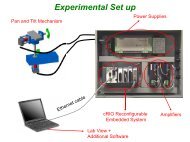
The learning control and NMPC algorithms have been applied to a rotary inverted pendulum testbed. The system
is nonlinear, underactuated, and unstable at the target state (vertical up position), making the system a challenging
candidate for control. The horizontal link is controlled to bring the vertical link upright. This is called the swing-up
control. The system model is included in Appendix B. In this section, we describe the physical hardware and software
environment that we have used to implement the learning and NMPC algorithms.
4.1 Hardware
The experiment was constructed as part of a kit in support of control education [19]. A MicroMo motor is used in
the driving joint. A 1024-count encoder is mounted on each joint. The open-loop control law is implemented on
a DSP control board made by ARCS, Inc. This board includes a TI C30 class processor and on-board A/D, D/A,
encoder, and digital I/O interfaces. The feedback NMPC control is implemented using MATLAB xPC Target with
Real-Time Workshop and Simulink Toolbox from MathWorks, Inc. The incremental encoder board is APCI-1710
from ADD-DATA, Inc., supporting 4 channels of single-ended/differential encoder with 32-bit resolution. The D/A
8

oard is PCIM-DAS1602/16 from Measurement Computing, Corp., which supports 2 16-bit D/A channels. The real-
time controlling PC is an AMD Athlon 1.4GHz with 512MB RAM.
4.2 Software
4.2.1 Simulation Model
Both learning control and NMPC have been extensively tested on the simulation model before applying to the physical
experiment. Simulink is used for the simulation study as well as for the real-time code generation by using the Real-
Time Workshop. In the Simulink model, the NMPC algorithm was programmed in C and converted into a Simulink
S-Function block by using the C-MEX S-Function Wrapper. This simulation environment allows us to tune the
controller parameters.
4.2.2 Real-Time Model
For the iterative learning control, an open-loop controller is coded using Simulink and compiled into C-code by using
the Real-Time Workshop (RTW). The state variables are logged for each run for the off-line control update. The
NMPC algorithm is also coded using Simulink and compiled using RTW.
4.2.3 Velocity Estimation
For the physical experiment, only the position variable is available (from the incremental encoders), and velocities
have to be estimated from the position measurement. For the open-loop control, velocities are estimated by simple
Euler approximation. For the NMPC control system, the washout filter is used. When the pendulum is near the
vertical equilibrium, a full order linear observer is used. A more detailed study of the effect of velocity estimation on
the performance of NMPC can be found in [20].
9

5 Experimental Results
5.1 Iterative Learning Control
Since for the learning control, the input is open-loop, real-time computation load is not an issue. Hence we choose a
longer prediction horizon:
T =1.5s, ts =5ms, M = T/ts = 300.
The number of Laguerre functions used is N =10and the Laguerre decaying factor, a, is chosen to be 0.9. For the
control penalty function, we choose
γ =0.45 umax =0.45N-m umin = −0.45N-m
We have observed that these parameters may vary significantly and still achieve swing-up and capture. The key
consideration is that ts should be chosen small enough to ensure sufficiently small discretization error and T should
be chosen large enough to allow swing-up with the specified control bound. Though the analytical model is not good
enough for direct open loop control, it appears to be adequate for generating a descent direction.
For the physical experiment, the initial control sequence is obtained using the algorithm described in Section 2.1.
However, the model/plant mismatch prevents the pendulum to be captured by the linear controller. After three iter-
ations using the gradient algorithm in Section 2.2, the linear controller is able to capture and balance the pendulum.
Figure 1 shows the experimental results using the control sequence obtained after the third iteration. The pendulum
link is shown to be swung up (i.e., x2 goes from −90 ◦ to 90 ◦ ) after two swings, and then captured and balanced by
the linear controller. Note that the control effort is well within the saturation limit.
5.2 NMPC
After tuning the controller parameters using simulation, we have settled with the choice of
M =80, T =0.4s, ts =5ms.
10

Again, these parameters may be adjusted and still achieve consistent swing-up. The parameter guide line is similar to
the iterative learning control case, ts should be small enough to limit the discretization error, T should be large enough
for the control bound to be satisfied. We have observed consistent swing-up and capture for T varying between
0.3 sec. and 0.45 sec., and ts varying between 4 ms and 6 ms. The number of swings (and hence the time to reach the
swing-up position) does vary with the choice of these parameters. The initial control vector is set to zero to minimize
the use of a priori information. The control constraint is imposed via a quadratic exterior penalty function described
in (7), with the parameters
γ =0.45, umax =0.1N-m, umin = −0.1N-m.
Note that the exterior penalty function does not ensure a hard bound on the input; therefore, a tighter control constraint
is chosen to satisfy the physical constraint of 0.45N-m. In both simulation and physical experiments, a hard saturation
constraint of ±0.45N-m is imposed for the control input.
The simulation result using the analytical model is shown in Figure 2. Note that the pendulum link initially moves
in the opposite direction as the iterative control result in Figure 1, since the initial control sequence is chosen to be
zero and it takes time for the control sequence to evolve through gradient modification in (15). After about 0.3 sec.,
the control and state trajectories become more similar to the open loop result in Figure 1. Four sample experimental
runs using the same controller parameters are shown in Figures 3-6. Even though the controller parameters are the
same, the response behaves differently after the pendulum is swung up. This is due to the lack of robustness in the
balanced configuration. In Figure 3-4, the pendulum remains balanced after swing-up, but in Figure 5-6, the pendulum
falls down at about 3 sec., in different directions, and then swings up again within 1 sec.
In all these experiments, the state trajectories in the swing-up phase match reasonably well with the simulation
prediction shown in Figure 7. The control trajectories show the same trend within the first second, but the experimental
responses contain much more chattering between the saturation levels when it is near the swung-up position (see
Figure 8). In general, the NMPC controller is very sensitive to disturbance during the balancing phase. It appears that
the 80-step horizon is too long at the balanced position for the controller to react effectively to the destabilizing effect
of the gravity. We have recently tried to adjust the length of the prediction horizon near the balancing position and had
some success [20]. This inability to maintain the balancing position may be attributed to several factors: modeling
error due to the vibration of the fixed support, the relatively poor velocity estimation (estimated through washout filter
11

in this implementation), and poor estimate of the Coulomb friction. When a linear observer based controller is used
near the balancing state, the experimental results shown in Figure 9–10 now very close to the simulation.
6 Conclusions
This paper presents the experimental implementation and results of iterative learning control and nonlinear model
predictive control applied to the swing-up of a rotary inverted pendulum with input torque constraint. In both cases,
computation load is reduced by using a Newton-step control update instead of solving the complete optimal control
problem. In the real-time control case with NMPC, MATLAB xPC-Target is used as the real-time computation plat-
form, and 5ms sampling rate is achieved with an 80-step look-ahead horizon. Coupled with a linear control law that
captures and balances the pendulum in the neighborhood of the vertical equilibrium, both iterative learning control
and NMPC control can swing up and balance the the pendulum consistently. Current work involves on improving the
robustness of NMPC and applying NMPC to the observer implementation.
Acknowledgment
This work is supported in part by the National Science Foundations under grant CMS-9813099, and in part by the
Center for Advanced Technology in Automation Technologies under a block grant from the New York State Science
and Technology Foundation.
12

References
[1] W. H. Kwon and A. E. Pearson. On feedback stabilization of time-varying discrete linear systems. IEEE Trans.
on Automatic Control, 23(3):479–481, June 1978.
[2] V. H. L. Cheng. A direct way to stabilize continuous-time and discrete-time linear time-varying systems. IEEE
Trans. on Automatic Control, 24(4):641–643, August 1979.
[3] C. C. Chen and L. Shaw. On receding horizon feedback control. Automatica, 18(3):349–352, 1982.
[4] S. S. Keerthi and E. G. Gilbert. Optimal infinite-horizon feedback laws for a general class of constrained discrete-
time systems : stability and moving-horizon approximation. Journal of Optimization Theory and Applications,
57(2):265–293, May 1988.
[5] D. Q. Mayne and H. Michalska. Receding horizon control of nonlinear system. IEEE Trans. on Automatic
Control, 35(7):814–824, July 1990.
[6] D. Q. Mayne and H. Michalska. Robust receding horizon control of constrained nonlinear system. IEEE Trans.
on Automatic Control, 38(11):1623–1633, November 1993.
[7] A. Jadbabaie, J. Yu, and J. Hauser. Receding horizon control of the caltech ducted fan: A control lyapunov
function approach. In Proc. 1999 IEEE Conference on Control Applications, 1999.
[8] S. L. Oliveira and M. Morari. Contractive model predictive control for constrained nonlinear systems. IEEE
Trans. on Automatic Control, 45(6):1053–1071, June 2000.
[9] F. Lizarralde, J. T. Wen, and L. Hsu. A new model predictive control strategy for affine nonlinear control systems.
In Proc. 1999 American Control Conference, pages 4263–4267, San Diego, CA, June 1999.
[10] A. Divelbiss and J. T. Wen. A path space approach to nonholonomic motion planning in the presence of obstacles.
IEEE Trans. on Robotic and Automation, 13(3):443–451, June 1997.
[11] N. Wiener. The theory of Prediction Modern Mathematics for Enginners. McGraw-Hill, 1956.
[12] B. Wahlberg. System identification using laguerre models. IEEE Trans. on Automatic Control, 36(5):551–562,
May 1991.
13

[13] C. C. Zervos and G. A. Dumont. Deterministic adaptive control based on laguerre series representation. Inter-
national Journal of Control, pages 2333–2359, 1988.
[14] L. Wang. Discrete time model predictive control design using laguerre functions. In Proceedings of 2001
American Control Conference, pages 2430–2435, Arlington, VA, 2001.
[15] E. Polak. Optimization: Algorithms and Consistent Approximations. Springer-Verlag, New York, 1997.
[16] E. D. Sontag. Control of systems without drift via generic loops. IEEE Trans. on Automatic Control, 40(7):1210–
1219, July 1995.
[17] D. Popa and J.T. Wen. Singularity computation for iterative control of nonlinear affine systems. Asian Journal
of Control, 2(2):57–75, June 2000.
[18] J.T. Wen and S. Jung. Nonlinear model predictive control based on the reduction of predicted state error. Tech-
nical report, Rensselaer Polytechnic Institute, Troy, NY, also available at http://www.cat.rpi.edu/˜
wen/papers/nmpc.pdf, July 2003.
[19] B. Potsaid and J.T Wen. Edubot: a reconfigurable kit for control education. part i. mechanical design. In Proc.
2000 IEEE International Conference on Control Applications, pages 50–55, 2000.
[20] J. Neiling. Nonlinear model predictive control of a rotary inverted pendulum. Master’s thesis, Rensselaer Poly-
technic Institute, Troy, NY., April 2003.
14

A Laguerre Functions used in Learning Control
In continuous time, the Laguerre function set is defined as:
fi(t) = e
2p
pt d
(i − 1)!
i−1
dti−1 [ti−1e −2pt ] (17)
where i is the order of the function set i =1, 2,...,N and p is Laguerre pole. The corresponding Laplace transform
for this set is:
Fi(s) = (s − p)i−1
2p
(s + p) i . (18)
The z-transform of the discrete Laguerre function set, li(k), i=1, 2,...,N is given in [12]:
Li(z) =
√ 1 − a 2
z − a
[az − 1
z − a ]i−1
Based on the z-transform, it is possible to the discrete Laguerre function set satisfies the difference equation
where
with initial condition
Lk =
Lk+1 =ΩLk
ψ1k ψ2k ... ψNk
⎡
⎢ a
⎢ a
⎢
Ω= ⎢
⎣
0 ... 0
2 − 1
a(a
a ... 0
2 − 1) a2 a
− 1 ... 0
2 (a2 − 1) a(a2 ···
a
− 1)
···
... 0
N−2 (a2 − 1) aN−3 (a2 ⎤
− 1) ...
⎥
⎦
a
T
L0 = 1 − a2
1 a a2 a3 ... aN−1 15
T
(19)
(20)

and discrete Laguerre pole a.
B Model of Rotary Inverted Pendulum
The rotary inverted pendulum used in this study is shown in Figure 11. The equation of motion is of the following
form:
M(θ) ¨ θ + C(θ, ˙ θ) ˙ θ + F ( ˙ θ)+G(θ) =Bu (21)
where θ, ˙ θ, ¨ θ are the joint angle, velocity and acceleration vectors, M(θ) is the mass-inertia matrix, C(θ, ˙ θ) ˙ θ is the
centrifugal and Coriolis torques, F ( ˙ θ) is the friction, G(θ) ∈R 2 is the gravity load, and u is the applied torque.
with
The inertia matrix is given by
m11 = m1l 2 c1 + I331
⎡
⎢
M(θ) = ⎢
⎣
m11 m12
m21 m22
2 + m2 l1 + l2 c2 cos2 (θ2) + I222 sin2 (θ2)+I332 cos2 (θ2)+2sin(θ2)cos(θ2) I232
m12 = m21 = −m2l1lc2 sin (θ2)+I122 sin (θ2)+I132 cos (θ2)
m22 = m2l 2 c2 + I112
C(θ, ˙ ⎡
⎢
θ)= ⎢
⎣
c11 c12
c21 c22
with
c11 = −2m2l2 c2 sin (θ2)cos(θ2) ˙ θ2 +2sin(θ2)cos(θ2)(I222 − I332 ) ˙
2
θ2 +I232 4cos (θ2) − 2 θ2
˙
c12 = −m2l1lc2 cos (θ2) ˙ θ2 + I122 cos (θ2) ˙ θ2 − I132 sin (θ2) ˙ θ2
c21 = m2l 2 c2 sin (θ2)cos(θ2) ˙ θ1 − I222 sin (θ2)cos(θ2) ˙ θ1 + I332 sin (θ2)cos(θ2) ˙ θ1 +I232
c22 =0
16
⎤
⎥
⎦
⎤
⎥
⎦
1 − 2cos 2 (θ2) ˙ θ1
(22)
(23)

The friction is modeled as Coloumb + viscous:
F ( ˙ ⎡
⎢ Fv1|
θ)= ⎢
⎣
˙ θ1| + Fc1sgn( ˙ θ1)
Fv2| ˙ θ2| + Fc2sgn( ˙ ⎤
⎥
⎦
θ2)
where Fv represent the coefficient of viscous friction for each joint, and Fc of Coulomb friction. For the NMPC
computation, we ignore the Coulomb friction terms due to the difficulty that discontinuity poses in gradient calculation.
The gravity term is
The torque is applied only on the first link, therefore
⎡
⎤
⎢
G(θ) = ⎢
⎣
0
m2glc2 cos (θ2)
⎥
⎦
⎡ ⎤
⎢
B = ⎢
⎣
1
0
⎥
⎦
For the state space representation, we define the state vector as
⎡ ⎤
⎢
x = ⎢
⎣
θ
p
⎥
⎦
where p ∆ = M(θ) ˙ θ is the generalized momentum. The equation of motion in the state space form is then
˙x =
⎡
⎢
⎣
M −1 (θ)p
( ˙ M(θ, M−1p) − C(θ, M−1p))M −1p − F (M −1p) − G(θ)
= f(x)+g(x)u.
The physical parameters are determined through direct measurements:
m1 =0.11409 kg l1 =0.169 m lc1 =0.1137 m
m2 =0.04474 kg l2 =0.162 m lc2 =0.0511 m
where subscripts 1 and 2 denote link 1 and link 2, respectively.
17
⎤
⎥
⎦ +
⎡
⎢
⎣
02×1
B
(24)
(25)
(26)
⎤
⎥
⎦ u (27)

The moment of inertia for each link can be computed using the above values:
I111 =2.62e-5 kg m2 I221 =3.59e-5 kg m2 I331 =3.43e-5 kg m2
I121 = I211 =0 I131 = I311 =1.29e-5 kg m2 I231 = I321 =0
I112 =1.87e-5 kg m 2 I222 =4.82e-6 kg m 2 I332 =1.86e-5 kg m 2
I122
= I212 =0 I132 = I312 =0 I232 = I322 =5.24e-6 kg m2
Identification of friction parameters of the inverted pendulum system was performed and are given as follows
Fv1 =0.11409N-m/rad/sec Fc1 =0.008N-m
Fv2 =0.0001N-m/rad/sec Fc2 =0.0N-m
18

Figures
states
states
control
100
0
−100
−200
State & Control trajectories : Open−Loop System, Experiment
−300
0 0.5 1 1.5 2 2.5 3 3.5 4 4.5 5
20
10
0
−10
−20
0 0.5 1 1.5 2 2.5 3 3.5 4 4.5 5
0.4
0.2
0
−0.2
−0.4
0 0.5 1 1.5 2 2.5
time (sec)
3 3.5 4 4.5 5
Figure 1: State and Control trajectories on the Open-Loop Control System: After Third Iteration
19
x1
x2
x3
x4

position
velocity
control
position
200
100
0
−100
State & Control trajectories
−200
0 0.5 1 1.5 2 2.5 3 3.5 4 4.5 5
20
10
0
−10
−20
0 0.5 1 1.5 2 2.5 3 3.5 4 4.5 5
0.5
0
−0.5
0 0.5 1 1.5 2 2.5
time (sec)
3 3.5 4 4.5 5
velocity
control
200
100
0
−100
Figure 2: Simulation Response with NMPC
State & Control trajectories
−200
0 0.5 1 1.5 2 2.5 3 3.5 4 4.5 5
20
10
0
−10
−20
0 0.5 1 1.5 2 2.5 3 3.5 4 4.5 5
0.5
0
−0.5
0 0.5 1 1.5 2 2.5
time (sec)
3 3.5 4 4.5 5
Figure 3: Experimental Response with NMPC: sample run #1
20
x
1
x
2
x
3
x
4
x
1
x
2
x
3
x
4

position
velocity
control
position
200
100
0
−100
State & Control trajectories
−200
0 0.5 1 1.5 2 2.5 3 3.5 4 4.5 5
20
10
0
−10
−20
0 0.5 1 1.5 2 2.5 3 3.5 4 4.5 5
0.5
0
−0.5
0 0.5 1 1.5 2 2.5
time (sec)
3 3.5 4 4.5 5
Figure 4: Experimental Response with NMPC: sample run #2
velocity
control
200
100
0
−100
State & Control trajectories
−200
0 0.5 1 1.5 2 2.5 3 3.5 4 4.5 5
20
10
0
−10
−20
0 0.5 1 1.5 2 2.5 3 3.5 4 4.5 5
0.5
0
−0.5
0 0.5 1 1.5 2 2.5
time (sec)
3 3.5 4 4.5 5
Figure 5: Experimental Response with NMPC: sample run #3
21
x
1
x
2
x
3
x
4
x
1
x
2
x
3
x
4

x 1 (deg)
80
60
40
20
0
−20
−40
position
velocity
control
200
100
0
−100
State & Control trajectories
−200
0 0.5 1 1.5 2 2.5 3 3.5 4 4.5 5
20
10
0
−10
−20
0 0.5 1 1.5 2 2.5 3 3.5 4 4.5 5
0.5
0
−0.5
0 0.5 1 1.5 2 2.5
time (sec)
3 3.5 4 4.5 5
Figure 6: Experimental Response with NMPC: sample run #4
State Trajectory Comparison for x(1)
exp 1
exp 2
exp 3
exp 4
simulation
−60
0 0.2 0.4 0.6 0.8 1
time (sec)
1.2 1.4 1.6 1.8 2
x 3 rad/sec
15
10
5
0
−5
State Trajectory Comparison for x(3)
exp 1
exp 2
exp 3
exp 4
simulation
−10
0 0.2 0.4 0.6 0.8 1
time (sec)
1.2 1.4 1.6 1.8 2
x 2 deg.
150
100
50
0
−50
−100
State Trajectory Comparison for x(2)
x
1
x
2
x
3
x
4
exp 1
exp 2
exp 3
exp 4
simulation
−150
0 0.2 0.4 0.6 0.8 1
time (sec)
1.2 1.4 1.6 1.8 2
x 4 rad/sec
15
10
5
0
−5
−10
−15
State Trajectory Comparison for x(4)
exp 1
exp 2
exp 3
exp 4
simulation
−20
0 0.2 0.4 0.6 0.8 1
time (sec)
1.2 1.4 1.6 1.8 2
Figure 7: Comparison of State Response
22

position
velocity
control
torque (N−m)
0.5
0.4
0.3
0.2
0.1
0
−0.1
−0.2
exp −0.3 1
exp 2
exp 3
exp −0.4 4
simulation
200
100
−100
Control Trajectory
−0.5
0 0.2 0.4 0.6 0.8 1
time (sec)
1.2 1.4 1.6 1.8 2
0
Figure 8: Comparison of Control Trajectory
State & Control trajectories
−200
0 0.5 1 1.5 2 2.5 3 3.5 4 4.5 5
20
10
0
−10
−20
0 0.5 1 1.5 2 2.5 3 3.5 4 4.5 5
0.5
0
−0.5
0 0.5 1 1.5 2 2.5
time (sec)
3 3.5 4 4.5 5
Figure 9: Experimental Response with NMPC + linear balancing control: sample run #1
23
x
1
x
2
x
3
x
4

position
velocity
control
200
100
0
−100
State & Control trajectories
−200
0 0.5 1 1.5 2 2.5 3 3.5 4 4.5 5
20
10
0
−10
−20
x
3
x
4
0 0.5 1 1.5 2 2.5 3 3.5 4 4.5 5
0.5
0
−0.5
0 0.5 1 1.5 2 2.5
time (sec)
3 3.5 4 4.5 5
Figure 10: Experimental Response with NMPC + linear balancing control: sample run #2
Figure 11: The Rotary Inverted Pendulum Experiment
24
x
1
x
2