

Lawrence et al., 2012: DRAFT: JGR: Ambient Noise Numerical ...
Lawrence et al., 2012: DRAFT: JGR: Ambient Noise Numerical ...
Lawrence et al., 2012: DRAFT: JGR: Ambient Noise Numerical ...

You also want an ePaper? Increase the reach of your titles
YUMPU automatically turns print PDFs into web optimized ePapers that Google loves.
<strong>Lawrence</strong> <strong>et</strong> <strong>al</strong>., <strong>2012</strong>: <strong>DRAFT</strong>: <strong>JGR</strong>: <strong>Ambient</strong> <strong>Noise</strong> Numeric<strong>al</strong> Ev<strong>al</strong>uation<br />
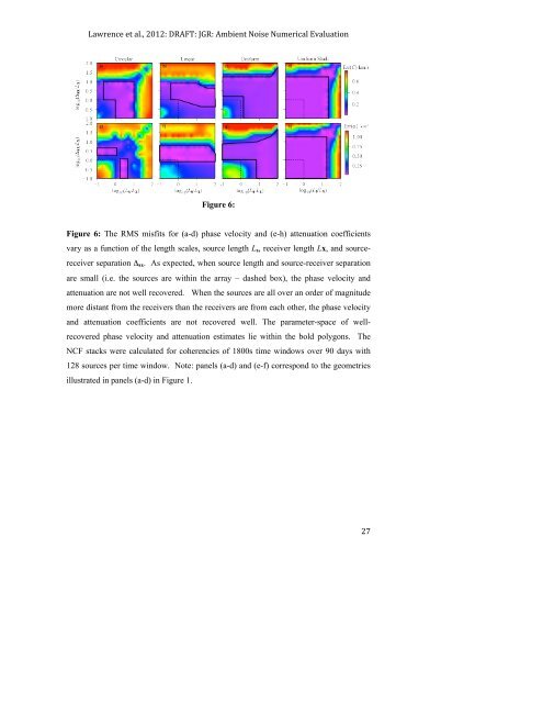
Figure 6:<br />
Figure 6: The RMS misfits for (a-d) phase velocity and (e-h) attenuation coefficients<br />
vary as a function of the length sc<strong>al</strong>es, source length Ls, receiver length Lx, and source-<br />
receiver separation Δsx. As expected, when source length and source-receiver separation<br />
are sm<strong>al</strong>l (i.e. the sources are within the array – dashed box), the phase velocity and<br />
attenuation are not well recovered. When the sources are <strong>al</strong>l over an order of magnitude<br />
more distant from the receivers than the receivers are from each other, the phase velocity<br />
and attenuation coefficients are not recovered well. The param<strong>et</strong>er-space of well-<br />
recovered phase velocity and attenuation estimates lie within the bold polygons. The<br />
NCF stacks were c<strong>al</strong>culated for coherencies of 1800s time windows over 90 days with<br />
128 sources per time window. Note: panels (a-d) and (e-f) correspond to the geom<strong>et</strong>ries<br />
illustrated in panels (a-d) in Figure 1.<br />
27


