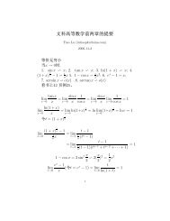
Abstract
Abstract
Abstract

Create successful ePaper yourself
Turn your PDF publications into a flip-book with our unique Google optimized e-Paper software.
Numerical Methods for the Wigner-Poisson Equations<br />
<strong>Abstract</strong><br />
LASATER, MATTHEW SCOTT. Numerical Methods for the Wigner-Poisson Equa-<br />
tions. (Under the direction of C.T. Kelley).<br />
This thesis applies modern numerical methods to solve the Wigner-Poisson equa-<br />
tions for simulating quantum mechanical electron transport in nanoscale semicon-<br />
ductor devices, in particular, a resonant tunneling diode (RTD). The goal of this<br />
dissertation is to provide engineers with a simulation tool that will verify earlier nu-<br />
merical results as well as improve upon the computational efficiency and resolution<br />
of older simulations. Iterative methods are applied to the linear and nonlinear prob-<br />
lems in these simulations to reduce the computational memory and time require to<br />
calculate solutions.<br />
Edited by Foxit PDF Editor<br />
Copyright (c) by Foxit Software Company, 2004<br />
For Evaluation Only.<br />
Initially the focus of the research involved updating time-integration techniques,<br />
but this switched to implementing continuation methods for finding steady-state so-<br />
lutions to the equations as the applied voltage drop across the device varied. This<br />
method requires the solution to eigenvalue problems to produce information on the<br />
RTD’s time-dependent behavior such as the development of current oscillation at a
particular applied voltage drop. The continuation algorithms/eigensolving capabili-<br />
ties were provided by Sandia National Laboratories’ software library LOCA (Library<br />
of Continuation Algorithms). The RTD simulator was parallelized, and a precondi-<br />
tioner was developed to speed-up the iterative linear solver. This allowed us to use<br />
finer computational meshes to fully resolve the physics.<br />
We also theoretically analyze the steady-state solutions of the Wigner-Poisson<br />
equations by noting that the solutions to the steady-state problem are also solutions<br />
to a fixed point problem. By analyzing the fixed point map, we are able to prove<br />
some regularity of the steady-state solutions as well provide a theoretical explanation<br />
for the mesh-independence of the preconditioned linear solver.<br />
October 5, 2005
NUMERICAL METHODS FOR THE<br />
WIGNER-POISSON EQUATIONS<br />
by<br />
Matthew S. Lasater<br />
a dissertation submitted to the graduate faculty of<br />
north carolina state university<br />
in partial fulfillment of the<br />
requirements for the degree of<br />
doctor of philosophy<br />
applied mathematics, computational mathematics concentration<br />
raleigh, north carolina<br />
October 2005<br />
approved by:<br />
C. T. Kelley<br />
chair of advisory committee<br />
P. A. Gremaud R. H. Martin<br />
M. Shearer D. L. Woolard
Biography<br />
Matthew Lasater was born on June 4th, 1980 in Gastonia, NC. He continued to live<br />
there until 1996, when he left to attend the North Carolina School of Science and<br />
Mathematics in Durham, NC. After graduating from NCSSM in May of 1998, he<br />
moved to Raleigh, NC to begin college at North Carolina State University. Being as<br />
fickle as he is, Matthew switched majors constantly during his time as an undergrad-<br />
uate, starting out as a computer science major, moving on to physics, then statistics,<br />
to finally graduating in June 2001 with his bachelors in applied mathematics. He<br />
started graduate school the following August at NCSU in applied mathematics with<br />
the intention of getting his masters in applied mathematics but was swayed by his<br />
numerical analysis teacher (and soon-to-be advisor) to complete a Ph.D. program<br />
instead. Earning his bachelors in physics with a minor in statistics in May 2002,<br />
Matthew is pressing on to finish his Ph.D. in computational mathematics by the fall<br />
of 2005, after which he will start his job at M.I.T. Lincoln Laboratory as a member<br />
of the technical staff.<br />
ii
Acknowledgments<br />
First and foremost, I want to thank my advisor Tim Kelley. I appreciate his guidance,<br />
candor, knowledge, and patience without which I would not have finished this thesis.<br />
I am grateful for all he has done for me.<br />
I also want to thank some other members of the research project from which this<br />
work derives: Dwight Woolard, Peiji Zhao, and Greg Recine. They have helped me<br />
understand the application side of my research and prepared me for future work on<br />
interdisciplinary research projects.<br />
I would like to thank Pierre Gremaud, Stephen Campbell, and Ilse Ipsen for their<br />
critiques in the graduate student numerical analysis seminar and for Dr. Ipsen’s<br />
communication class. These have strengthened my ability to speak and write about<br />
mathematical topics and gave me a better appreciation of the pedagogical value found<br />
in these tasks.<br />
I am extremely thankful for the opportunity to intern at Sandia National Lab-<br />
oratories for two summers, and I want to thank Andy Salinger, Eric Phipps, Roger<br />
Pawlowski, Todd Coffey, Heidi Thornquist, and Robert Hoekstra for all their help at<br />
iii
Sandia. I was able to get a better understanding of the type of work mathematicians<br />
do at a government lab and would not have been as successful at incorporating LOCA<br />
into the RTD simulation as well as parallelizing the RTD simulation without their<br />
help.<br />
Eric Sills and Gary Howell deserve many thanks for answering my numerous com-<br />
puter questions and installing Trilinos (several times) on a cluster of computers at<br />
N.C. State University. I also want to thank Denise Seabrooks, Brenda Currin, Rory<br />
Loycano, Lesa Denning, and Mary Byrd for helping me through all the red tape and<br />
administrative processes involved with the graduate school. I would also like to thank<br />
my fellow graduate students Quinton Anderson, Todd Coffey, Dan Finkel, Katie Ka-<br />
vanagh Fowler, Nathan George, Rachel Levy, and Jill Reese for helping me through<br />
classes and showing me the ropes with using Matlab and LaTex.<br />
I want to thank my mom, dad, and brother Michael and my close friends Bill<br />
Bryan, Danielle Parker, and Jeremy Slatton for all their support through graduate<br />
school. Finally, my girlfriend Myra Durham’s daily care and devotion helped me keep<br />
my sanity when school was daunting and taxing, and I will forever appreciate her for<br />
that.<br />
iv
Table of Contents<br />
List of Tables ix<br />
List of Figures x<br />
1 Overview 1<br />
1.1 Introduction................................ 1<br />
1.2 Simulating Nanoscale Semiconductors . . . . . . . . . . . . . . . . . . 2<br />
1.3 QuantumMechanics ........................... 7<br />
1.4 QuantumStatisticalMechanics ..................... 10<br />
1.5 TheWigner-PoissonEquations ..................... 17<br />
1.6 Numerical Solution: Finite Difference Method . . . . . . . . . . . . . 21<br />
2 Temporal Integration 28<br />
2.1 IntegratorSelection............................ 28<br />
2.2 Newton-KrylovMethods ......................... 32<br />
2.3 GMRES:Matrix-FreeKrylovMethod.................. 34<br />
v
2.4 Preconditioning.............................. 37<br />
2.5 GlobalConvergence............................ 38<br />
2.6 PreconditionerDevelopment....................... 39<br />
2.7 Calculating Equilibrium Wigner Function . . . . . . . . . . . . . . . . 40<br />
3 Bifurcation Analysis 44<br />
3.1 Stability of Nonlinear Dynamics . . . . . . . . . . . . . . . . . . . . . 44<br />
3.2 Illustrative Examples . . . . . . . . . . . . . . . . . . . . . . . . . . . 46<br />
3.3 ContinuationMethods .......................... 50<br />
3.4 Linear Solver Methods for Pseudo Arc-Length Continuation . . . . . 53<br />
3.5 BorderingAlgorithms........................... 55<br />
3.6 HouseholderContinuation ........................ 56<br />
3.7 ParallelizationofSimulator ....................... 57<br />
3.8 Linear Solver Comparison for Pseudo Arc-Length Continuation . . . . 62<br />
3.9 Results................................... 64<br />
3.10CorrelationLengthStudy ........................ 68<br />
3.10.1 CurrentVoltageRelationship .................. 68<br />
3.10.2 Stability Analysis . . . . . . . . . . . . . . . . . . . . . . . . . 72<br />
4 Theory 74<br />
4.1 Steady-StateTheory ........................... 74<br />
4.2 Infinite-DimesionalAnalysisofGMRES................. 104<br />
vi
4.3 ApplicationofSchauder’sFixedPointTheorem ............ 110<br />
5 Conclusion 114<br />
References 117<br />
A Notation 123<br />
B Trilinos 131<br />
B.1 Introduction................................ 131<br />
B.2 Procedural and Object-Oriented Programming . . . . . . . . . . . . . 132<br />
B.3 Trilinos Packages . . . . . . . . . . . . . . . . . . . . . . . . . . . . . 134<br />
B.3.1 Epetra............................... 134<br />
B.3.2 LOCA............................... 135<br />
B.3.3 NOX................................ 135<br />
B.3.4 AztecOO.............................. 135<br />
B.3.5 Anasazi .............................. 136<br />
B.4 Contribution................................ 136<br />
C Guide to RTD Simulation Code 140<br />
C.1 InitializationCode ............................ 141<br />
C.1.1 equil.f . . . . . . . . . . . . . . . . . . . . . . . . . . . . . . . 141<br />
C.1.2 transi.f............................... 141<br />
C.1.3 wprockinit.f ............................ 141<br />
vii
C.1.4 homer.f .............................. 142<br />
C.2 ContinuationCode ............................ 142<br />
C.2.1 RTDProblemInterface.H ..................... 142<br />
C.2.2 RTDProblemInterfaceParallel.C................. 143<br />
C.2.3 RTDContinuationParallel.C . . . . . . . . . . . . . . . . . . . 143<br />
C.2.4 rtdrespara.f ............................ 145<br />
C.2.5 rtdinit1.f.............................. 146<br />
C.2.6 rtdinit2.f.............................. 146<br />
C.2.7 transipara.f ............................ 146<br />
C.2.8 dout.f ............................... 146<br />
C.3 DataFiles................................. 147<br />
C.3.1 grid.h ............................... 147<br />
C.3.2 material.dat............................ 147<br />
C.4 Compiling and Running The Simulation . . . . . . . . . . . . . . . . 147<br />
D GMRES and Arnoldi Iterative Methods 150<br />
viii
List of Tables<br />
1.1 PhysicalConstants ............................ 18<br />
2.1 SweepInBiasTiming .......................... 31<br />
2.2 Initialization Timings Newton-GMRES(800) . . . . . . . . . . . . . . 42<br />
2.3 Initialization Timings Preconditioned Newton-GMRES(100) . . . . . 42<br />
3.1 ComputationofParallelEfficiency.................... 59<br />
3.2 Scalability of RTD Simulation . . . . . . . . . . . . . . . . . . . . . . 60<br />
3.3 Comparison of Bordering and Householder Methods . . . . . . . . . 63<br />
3.4 Eigenvalue Calculations for 20 Percent Reduced Correlation Length . 73<br />
4.1 Krylov and Newton Iterations as Mesh Is Refined . . . . . . . . . . . 109<br />
4.2 PhysicalConstants ............................ 113<br />
ix
List of Figures<br />
1.1 Drawing of a Resonant Tunneling Diode and Its Electric Potential U 4<br />
1.2 Boundary Conditions on Wigner Distribution f ............ 27<br />
1.3 Grid Showing Modification of Composite Trapezoidal Rule . . . . . . 27<br />
2.1 Flow Chart for Computing U ...................... 28<br />
3.1 Steady-State Solution Branch of dw<br />
dt = h(w, α) =w2 − α ....... 47<br />
3.2 Steady-State Solution Branch of dw<br />
dt = h(w, α) =w3 − αw ...... 48<br />
3.3 Illustration of Pseudo-Arc Length Continuation . . . . . . . . . . . . 53<br />
3.4 Current-VoltagePlot ........................... 62<br />
3.5 Enlarged Portion of Curve Where Methods Were Compared . . . . . 63<br />
3.6 I-V Curve Generated by Time-Accurate Simulation . . . . . . . . . . 65<br />
3.7 Bias Window of Current Oscillation . . . . . . . . . . . . . . . . . . . 65<br />
3.8 I-VCurveGeneratedbyLOCA ..................... 66<br />
3.9 Eigenvalues Creating Oscillatory Solutions . . . . . . . . . . . . . . . 67<br />
3.10 Comparison of Current-Voltage Plots for Varying Grids . . . . . . . . 68<br />
x
3.11 I-V Curve with 30 Percent Reduced Correlation Length . . . . . . . . 69<br />
3.12 I-V Curve with 25 Percent Reduced Correlation Length . . . . . . . . 70<br />
3.13 I-V Curve with 20 Percent Reduced Correlation Length . . . . . . . . 70<br />
3.14 I-V Curve with 10 Percent Increased Correlation Length . . . . . . . 71<br />
3.15 I-V Curve with 20 Percent Increased Correlation Length . . . . . . . 71<br />
xi
Chapter 1<br />
Overview<br />
1.1 Introduction<br />
This thesis derives from research on enhancing the computation of Wigner-Poisson<br />
simulations. The Wigner-Poisson equations model electron transport that is domi-<br />
nated by quantum mechanics. This is applicable to devices that are designed on the<br />
nanoscale (10 −9 meters), which is the motivation for the research. The research was<br />
funded by the U.S. Army Research Office to understand and control the quantum<br />
mechanical effects that will be present when devices are scaled down to such a tiny<br />
size.<br />
The prototypical nanoscale semiconductor device under investigation in this work<br />
is a resonant tunneling diode (RTD). Numerical simulation [40], [41] have predicted<br />
terahertz (THz) frequency current oscillation in these devices. Terahertz radiation is<br />
1
CHAPTER 1. OVERVIEW 2<br />
being heavily researched by the U.S. Army for homeland security reasons [38], [39],<br />
and devices that operate on or could control terahertz frequency signals would be of<br />
special interest to the U.S. Army. These computer simulations [40], [41] took several<br />
days and were not accurate enough to resolve all the relevant physical processes. To<br />
get a complete understanding of the device, numerous more accurate runs are re-<br />
quired, but the computational requirement in time and resources was too great for<br />
the engineers when using their code. My research involved updating the code used<br />
for the simulation to modern nonlinear solvers in a parallel processing environment,<br />
using continuation methods and eigensolvers to effectively determine the onset of os-<br />
cillatory behavior in a parameter study, theoretically proving that the preconditioner<br />
used in computing steady-state distribution is mathematical scalability, and getting<br />
a regularity result for these steady-state distributions.<br />
1.2 Simulating Nanoscale Semiconductors<br />
Semiconductor technology has developed to the point where the next generation of<br />
electronic devices will operate at the nanoscale. Since the device scale is so small,<br />
design problems arise immediately. Currently, we do not have the technology to ob-<br />
serve and collect all relevant data from such small devices. Futhermore, even if we<br />
had this capability, the device physics are determined by quantum mechanics and<br />
not by classical electromagnetism. A fundamental result of quantum mechanics is<br />
that the act of observing a quantum system will have an impact on the results we
CHAPTER 1. OVERVIEW 3<br />
obtain. Thus, physically measuring how a normal quantum system is functioning<br />
would require an account of the effects of the observer on the reported data. To avoid<br />
this issue, engineers and physicists researching these quantum devices derive and use<br />
accurate models of these quantum systems from first-principle physics.<br />
In this work, we develop and analyze numerical methods for solving the Wigner-<br />
Poisson equations. These equations describe the statistical mechanics of particles<br />
under the influence of quantum mechanics. A classical analogue to the Wigner equa-<br />
tion is the Boltzmann equation [11] for describing the statistical mechanics of gas<br />
particles or electrons on the macroscale. The Wigner-Poisson equations consist of<br />
two equations: the Wigner distribution equation, a nonlinear integro-partial differ-<br />
ential equation which describes electron transport on the quantum level, coupled to<br />
Poisson’s equation, which determines the potential created by the electrons. In the<br />
past two decades, the Wigner-Poisson equations have been used to predict the be-<br />
havior of nanoscale semiconductor devices [14],[22]. One particular nanostructure we<br />
are interested in is the resonant-tunneling diode (RTD).<br />
Recently, resonant tunneling diodes have been considerably researched in the field<br />
of semiconductor technology [35], [36], [8]. Figure 1.1 shows a diagram of a RTD and<br />
the electric potential within the RTD.<br />
A RTD is created by the joining together two different semiconductors, material I<br />
and material II semiconductors. In a semiconductor material, the state of an electron<br />
is determined by its energy. If an electron has enough energy, then it is able to move
CHAPTER 1. OVERVIEW 4<br />
Doping Spacer Barrier Well Barrier Spacer Doping<br />
U(0)=0<br />
I<br />
II I II I<br />
x=0 x=L<br />
U(L)=−V<br />
V volts<br />
Figure 1.1: Drawing of a Resonant Tunneling Diode and Its Electric Potential U<br />
within the material. The minimum energy required for an electron to freely move<br />
about is material dependent. Semiconductor II is chosen so that it has a higher re-<br />
quired energy than semiconductor I. For our particular application we are studying,<br />
semiconductor I is gallium arsenide (GaAs) and semiconductor II is gallium aluminum<br />
arsenide (GaAlAs). The difference in minimum energies of the two materials creates<br />
potential barriers within the RTD. These barriers are shown in the electric potential<br />
which jumps up in the material II regions. Towards the two ends of the RTD, the<br />
semiconductor is doped (represented by the darkened area). Doping is where atoms<br />
that contain more (or fewer) electrons than the semiconductor itself are placed into<br />
the semiconductor to add (or take away) extra electrons in the structure. Between<br />
the barriers and the doped areas are regions of material I called spacers and trapped<br />
between the barrier is a region of material I semiconductor which is the quantum well
CHAPTER 1. OVERVIEW 5<br />
of the system.<br />
By putting different voltages at both ends of the device, (shown in the diagram by<br />
the voltage drop of V volts) electrons are attracted to one side of the device. Classi-<br />
cally, an electron is treated as a particle, and if a particle runs into a potential barrier,<br />
it is reflected back if the particle does not have enough momentum to overcome the<br />
barrier. In quantum mechanics though, electrons are treated as waves, and no matter<br />
how slowly the electrons are traveling, they still have some probability of crossing<br />
through the barriers. This effect is known as quantum tunneling, and it is the basic<br />
premise behind the device.<br />
Physical experiments in the 1980’s have shown current oscillation can be expected<br />
in the RTD [36]. To control this oscillation, engineers have used external circuit con-<br />
figurations, but the power produced by the RTDs in these configuration is not large<br />
enough to be useful [42]. Engineers are now looking at trying to control these oscil-<br />
lations by intrinsic means in hopes of producing larger power output from the RTD.<br />
Numerical simulations [40],[41] have shown that current oscillation can be in the THz<br />
range. With these numerical simulations, engineers hope they can determine what<br />
physical parameters (i.e., doping profile, barrier height and width, well width, etc.)<br />
are conducive to sustaining and controlling these oscillations,in hopes of producing a<br />
viable high frequency power source.<br />
Terahertz devices have great potential for computational and military applica-<br />
tions. There is ongoing research [38], [39] for using terahertz radiation for detecting
CHAPTER 1. OVERVIEW 6<br />
and identfying biological and chemical warfare agents. In a battlefield environment,<br />
the ability to remotely detect biological and chemical warfare agents would reduce the<br />
risk of injuries and casualties. Also, computational efficiency and data transmission<br />
will be greatly increased once sustainable terahertz frequencies are possible. The goal<br />
of this research is to create a numerical tool for engineers and scientists to use in order<br />
to understand the physical mechanisms behind the RTD’s operation and potentially<br />
exploit these mechanisms to create terahertz frequency devices.<br />
The problem of numerically simulating nanoscale semiconductor devices with the<br />
Wigner formalism is an active field of research. The numerical method we use is a<br />
finite-difference approximation as described in [8]. Other discretizations can be used.<br />
In [32], [31], the author considers using a spectral discretization. Here, functions<br />
are approximated by a truncated Fourier series, where the coefficients on the finite-<br />
dimensional Fourier basis are computed. In [32], the author proposed a mixed finite<br />
difference-spectral method (differences in x and t space, spectral in k space) for the<br />
coupled Wigner-Poisson equations. This is for a bounded domain in one-dimensional<br />
x space, with time-dependent Dirchlet boundary conditions. In the paper, the author<br />
derives errors estimations and establishes consistency of the method, gets a priori nu-<br />
merical bounds on the solution, and presents numerical results. The author, though,<br />
do not account for scattering effects that will occur within the semiconductor. This<br />
was an extension of [31], where the author only considered the linear Wigner equation<br />
(i.e. no coupling with Poisson’s equation, only a fixed potential U is given). A reason
CHAPTER 1. OVERVIEW 7<br />
this work in not applicable to the device we are studying is that the potential has to<br />
be sufficiently smooth to guarantee convergence of the method, and we are simulating<br />
devices with discontinuous potentials.<br />
Another method of solving this problem numerically is using a particle method.<br />
In [4], the authors propose applying a weighted particle method. Here, particles<br />
are tracked in (x, k) space as they move according to the Wigner equation and the<br />
approximate solution we obtain is a weigted sum of delta functions involving the par-<br />
ticles. Note, these particles should be thought of in a mathematical sense, and are<br />
not physical particles. This method is particularly relevant to our problem, because<br />
in this paper, the authors show convergence of this method not only for a smooth<br />
potential U but also for a discontinuous U that contains potential barriers, which is<br />
the physical case we are attempting to model. The authors only consider the linear<br />
Wigner equation with a fixed potential U and neglect scattering effects that will be<br />
present.<br />
1.3 Quantum Mechanics<br />
Since the device we are studying exists on the nanoscale, the model we use must<br />
accurately account for quantum mechanical effects. In classical physics, actions are<br />
inherently deterministic. That is, given a particle’s position, velocity, mass, forces act-<br />
ing on it, etc. we can accurately calculate its trajectory for any future time. Classical<br />
physics (Newtonian mechanics and classical electromagnetism) is a powerful method
CHAPTER 1. OVERVIEW 8<br />
for predicting the actions of objects that are of moderate size (that is, objects that<br />
are not as large as galaxies but are not as small as atoms).<br />
Quantum mechanics, though, is a probabilistic description of nature. The fun-<br />
damental idea of quantum mechanics is that matter exhibits a wave-particle duality.<br />
This means matter acts in some respects as both a particle and a wave. For a particle<br />
in classical mechanics, we can describe its instantaneous state by giving its position<br />
and velocity. In quantum mechanics [26],[23], to describe a particle’s instantaneous<br />
state, we need an object called a wavefunction. We will now list some postulates of<br />
quantum mechanics. For these postulates, we are considering just a single particle<br />
and not a system of particles, and these particles are confined to move in one space<br />
dimension. These postulates can be easily extended to a more general case:<br />
1. The quantum state of a particle is described by a wavefunction ψ(x) whichis<br />
an element of the complex Hilbert space L 2 . A physical interpretation of the<br />
wavefunction is as probability distribution, where the probability of finding a<br />
particle in a region dx about the point x is given by |ψ(x)| 2 dx. Since the particle<br />
must exist somewhere in (−∞, ∞), this imposes the normalization condition<br />
that ∞<br />
−∞ |ψ(x)|2 dx =1.<br />
2. Every physical observable quantity has a linear, Hermitian operator associated<br />
with it. Further, for a given operator Θ, we can calculate its expected value
CHAPTER 1. OVERVIEW 9<br />
(which will be denoted by < Θ >) for the state ψ(x) by the formula<br />
< Θ >=<br />
∞<br />
−∞<br />
ψ ∗ (x)Θψ(x)dx<br />
Here, ψ ∗ (x) denotes the complex-conjugate of ψ(x). For example, if the wave-<br />
functions are in terms of position, the operator of position is x and the operator<br />
for momentum is p = −i ∂<br />
h<br />
,where = and h is Planck’s constant. So the<br />
2π ∂x<br />
expected position of the electron would be<br />
=<br />
∞<br />
−∞<br />
ψ ∗ (x)xψ(x)dx =<br />
∞<br />
−∞<br />
and the expected momentum of the electron would be<br />
=<br />
∞<br />
−∞<br />
x|ψ(x)| 2 dx<br />
ψ ∗ (x)(−i ∂<br />
∞<br />
)ψ(x)dx = −i ψ<br />
∂x −∞<br />
∗ (x) ∂ψ(x)<br />
∂x dx<br />
For a given potential field U(x), the total energy operator, called the Hamilto-<br />
nian operator, is given by H = p2<br />
2m∗ + U(x), where m∗ istheeffectivemassof<br />
the electron. Since p = −i ∂<br />
, then the Hamiltonian operator can be written<br />
as H = −2<br />
2m ∗<br />
∂2 + U(x).<br />
∂x2 ∂x<br />
3. While determining the exact future position and speed of an electron is impos-<br />
sible, the evolution of the electron’s wavefunction is deterministic and is given
CHAPTER 1. OVERVIEW 10<br />
by Schrödinger’s Equation (in one dimension):<br />
i ∂ψ<br />
∂t<br />
= Hψ = −2<br />
2m ∗<br />
∂2ψ + U(x)ψ. (1.1)<br />
∂x2 The above wavefunction is a function of the electron’s position. There is another<br />
corresponding wavefunction, φ(p), that contains the same information as ψ(x), but<br />
in terms of the electron’s momentum p instead of its position. These wavefunctions<br />
are related through the Fourier transform by (in one space dimension)<br />
φ(p) =<br />
∞<br />
−∞<br />
ψ(x)e −ipx<br />
dx<br />
The momentum of an electron can also be represented by its wave number k, where<br />
p = k. There are also constraints on the wavefunction ψ(x) which must be satisfied.<br />
These include:<br />
• ψ(x) is continuous.<br />
• If the potential field U(x) is continuous, then ∂ψ(x)<br />
∂x is also continuous.<br />
• limx→∞ ψ(x) = limx→−∞ ψ(x) =0.<br />
1.4 Quantum Statistical Mechanics<br />
While the wavefunction formalism of quantum mechanics is useful for looking at one<br />
electron, it is not as helpful for investigating several electrons that can be existing
CHAPTER 1. OVERVIEW 11<br />
in many different states at once. While one could write a wavefunction that would<br />
describe the state of the ensemble of electrons, the wavefunction would be written<br />
as ψ(¯x1, ¯x2,...,¯xn), where ¯xi would be the spatial coordinate of the ith electron.<br />
This becomes quite computationally burdensome when dealing with more than a few<br />
electrons. Therefore, other formalisms of quantum mechanics would be better suited<br />
to handle the description of an ensemble of electrons. One such formalism is the<br />
density matrix formalism [5], [12]. The Wigner function is derived from the density<br />
matrix, so we shall first explain the density matrix.<br />
Let {ψi(q)} be a collection of the possible states which the electrons can exists and<br />
{¯ji} be the corresponding probabilites that an electron is found in these states. The<br />
density matrix stores all this information into one compact form. The density matrix<br />
is a function of two position variables and is given by ρ(q, r) = <br />
i ¯jiψi(q)ψ ∗ i (r). The<br />
time evolution of the density matrix can be derived from Schrödinger’s equation as<br />
follows:<br />
∂ρ(q, r)<br />
∂t<br />
∂ <br />
=<br />
∂t<br />
i<br />
= ∂<br />
¯ji<br />
i<br />
¯jiψi(q)ψ ∗ i (r)<br />
∂t [ψi(q)ψ ∗ i (r)]<br />
= <br />
¯ji[ ∂ψi(q)<br />
Schrödinger’s equation tells us that ∂ψ(q)<br />
∂t<br />
i<br />
∂t ψ∗ i (r)+ψi(q) ∂ψ∗ i (r)<br />
∂t<br />
1<br />
=<br />
i [−2<br />
2m∗ ∂2ψ(q) ∂q2 +U(q)ψ(q)] and ∂ψ∗ (r)<br />
∂t =<br />
− 1<br />
i [−2<br />
2m∗ ∂2ψ ∗ (r)<br />
∂r2 + U(r)ψ∗ (r)]. Substituting these into the above equation and rear-<br />
]
CHAPTER 1. OVERVIEW 12<br />
ranging terms gives the simplified expression:<br />
∂ρ(q, r)<br />
i<br />
∂t<br />
2<br />
= −<br />
2m<br />
∂q<br />
∂2 ∂2<br />
( − ∗ 2<br />
)ρ(q, r)+[U(q) − U(r)]ρ(q, r) (1.2)<br />
∂r2 The Wigner distribution can be derived from the density matrix [15]. First, we<br />
change the cooridinates of the density matrix from (q, r) to(x, y) byx = 1<br />
(q + r)<br />
2<br />
and y = q − r. Soq = x + 1<br />
1<br />
y and r = x − y. The Wigner distribution is defined as<br />
2 2<br />
f(x, p) =<br />
∞<br />
−∞<br />
dyρ(x + 1<br />
2<br />
1 −ipy<br />
y, x − y)e (1.3)<br />
2<br />
The time evolution of the Wigner distribution f can be derived from (1.2) and (1.3).<br />
We note that<br />
∂<br />
∂q<br />
=<br />
∂x ∂ ∂y ∂ 1 ∂<br />
+ =<br />
∂q ∂x ∂q ∂y 2 ∂x<br />
∂<br />
∂r<br />
=<br />
∂x ∂ ∂y ∂ 1 ∂<br />
+ =<br />
∂r ∂x ∂r ∂y 2 ∂x<br />
Using both of these facts, we have that<br />
∂ 2<br />
∂q<br />
2 − ∂2<br />
=(∂<br />
∂r2 ∂q<br />
∂<br />
+<br />
∂y<br />
∂<br />
−<br />
∂y<br />
∂ ∂ ∂<br />
+ )( −<br />
∂r ∂q ∂r )=(∂<br />
∂ ∂2<br />
)(2 )=2<br />
∂x ∂y ∂x∂y
CHAPTER 1. OVERVIEW 13<br />
So, we have from (1.2) and (1.3)<br />
where<br />
and<br />
∂f(x, p)<br />
∂t<br />
= ∂<br />
∂t<br />
=<br />
−∞<br />
∞<br />
dy<br />
dyρ(x + 1<br />
2<br />
−∞<br />
∞<br />
1 ∂ρ(x + 2<br />
= A(ρ)+B(ρ)<br />
A(ρ) =− <br />
im∗ ∞<br />
dy[<br />
−∞<br />
∂2<br />
∂x∂y<br />
B(ρ) = 1<br />
∞<br />
i −∞<br />
dy[U(x + 1<br />
2<br />
1 −ipy<br />
y, x − y)e <br />
2<br />
1 y, x − 2y) ∂t<br />
ρ(x + 1<br />
2<br />
y) − U(x − 1<br />
2<br />
We want to analyze A(ρ). First, we notice that<br />
Since<br />
∂<br />
∂y<br />
∞<br />
−∞<br />
[ρ(x + 1<br />
2<br />
dy[ ∂2<br />
∂x∂y<br />
ρ(x + 1<br />
2<br />
1 −ipy<br />
y, x − y)e ]=(<br />
2 ∂<br />
∂y<br />
then by (1.3) we have that<br />
∞<br />
−∞<br />
dy ∂<br />
∂y<br />
[ρ(x + 1<br />
2<br />
e −ipy<br />
<br />
1 −ipy<br />
y, x − y)]e <br />
2<br />
y)]ρ(x + 1<br />
2<br />
1 −ipy<br />
y, x − y)]e =<br />
2 ∂<br />
∞<br />
dy[<br />
∂x −∞<br />
∂<br />
∂y<br />
ρ(x + 1<br />
2<br />
∞<br />
1 −ipy<br />
y, x − y)e ]= dy[<br />
2 −∞<br />
∂<br />
∂y<br />
1 −ipy<br />
y, x − y))e<br />
2<br />
ρ(x + 1<br />
2<br />
1 −ipy<br />
y, x − y)e <br />
2<br />
ρ(x + 1<br />
2<br />
− ip 1<br />
ρ(x +<br />
2<br />
1 −ipy<br />
y, x − y)]e<br />
2<br />
1 −ipy<br />
y, x − y)]e <br />
2<br />
1 −ipy<br />
y, x − y)e <br />
2<br />
− ip<br />
f(x, p)
CHAPTER 1. OVERVIEW 14<br />
But because limy→∞ ρ(x + 1 1 y, x − 2<br />
2y) = 0 and limy→−∞ ρ(x + 1<br />
2<br />
y, x − 1<br />
2 y)=0since<br />
for any wavefunction ψ(q) wehavethatlimq→∞ ψ(q) = limq→−∞ ψ(q) = 0, we also<br />
know that<br />
∞<br />
−∞<br />
dy ∂<br />
∂y<br />
Therefore, we can conclude that<br />
∞<br />
−∞<br />
dy[ ∂<br />
∂y<br />
Placing this into A(ρ), we have<br />
[ρ(x + 1<br />
2<br />
ρ(x + 1<br />
2<br />
1 −ipy<br />
y, x − y)e ]=0<br />
2<br />
1 −ipy<br />
y, x − y)]e<br />
2<br />
= ip<br />
f(x, p)<br />
<br />
A(ρ) =− <br />
im∗ ∂<br />
∂x [ip<br />
p<br />
f(q, p)] = −<br />
m∗ ∂f(x, p)<br />
∂x<br />
Now we want to analyze B(ρ). First, by Fourier transforms, we have that<br />
So we have that<br />
B(ρ) = 1<br />
∞<br />
i<br />
−∞<br />
∞<br />
= 1<br />
i<br />
= 1<br />
2iπ2 ρ(x + 1<br />
2<br />
dy[U(x + 1<br />
2<br />
−∞<br />
∞<br />
dp<br />
−∞<br />
′ f(x, p ′ ∞<br />
)<br />
−∞<br />
∞<br />
1 1<br />
y, x − y)= dpf(x, p)e<br />
2 2π −∞<br />
ipy<br />
<br />
1 1 1 −ipy<br />
y) − U(x − y)]ρ(x + y, x − y)e <br />
2 2 2<br />
dye −ipy<br />
[U(x + 1<br />
∞<br />
1 1<br />
y) − U(x − y)](<br />
2 2 2π −∞<br />
p−p′<br />
−iy<br />
dye [U(x + 1<br />
1<br />
y) − U(x −<br />
2 2 y)]<br />
dp ′ f(x, p ′ )e ip′ y<br />
)
CHAPTER 1. OVERVIEW 15<br />
Now we will look at 0<br />
p−p′<br />
dye−iy<br />
−∞<br />
coordinates s = −y, wehavethat<br />
0<br />
−∞<br />
[U(x + 1<br />
p−p′<br />
−iy<br />
dye [U(x + 1<br />
1<br />
y) − U(x − y)] =<br />
2 2<br />
So we can conclude that<br />
0<br />
−∞<br />
p−p′<br />
−ir<br />
dye [U(x + 1<br />
1<br />
y) − U(x − y)] = −<br />
2 2<br />
2<br />
1<br />
y) − U(x − y)]. If we use the change of<br />
2<br />
∞<br />
0<br />
∞<br />
0<br />
p−p′<br />
is<br />
dse [U(x − 1<br />
1<br />
s) − U(x +<br />
2 2 s)]<br />
p−p′<br />
ir<br />
dye [U(x + 1<br />
1<br />
y) − U(x −<br />
2 2 y)]<br />
Therefore, for the inner integral in B(ρ), we get that ∞<br />
p−p′<br />
dye−iy [U(x + −∞ 1y)<br />
− 2<br />
U(x − 1<br />
2y)] equals ∞<br />
∞<br />
−∞<br />
p−p′<br />
−iy<br />
dye<br />
Finally, we have<br />
0<br />
p−p′<br />
p−p′<br />
iy dy[e−iy − e<br />
[U(x + 1<br />
1<br />
y) − U(x − y)] =<br />
2 2<br />
B(ρ) = 1<br />
2iπ2 ∞<br />
−∞<br />
= − 1<br />
π2 ∞<br />
dp ′ f(x, p ′ ∞<br />
)<br />
0<br />
dp<br />
−∞<br />
′ f(x, p ′ ∞<br />
)<br />
0<br />
][U(x + 1<br />
∞<br />
0<br />
dy[−2i sin(y<br />
2<br />
dy[2i sin(y<br />
1<br />
y) − U(x − y)]. So<br />
2<br />
p − p′<br />
<br />
p − p′<br />
<br />
)][U(x + 1<br />
1<br />
y) − U(x −<br />
2 2 y)]<br />
1<br />
1<br />
)][U(x + y) − U(x −<br />
2 2 y)]<br />
dy[U(x + 1<br />
1 p − p′<br />
y) − U(x − y)][sin(y<br />
2 2 )]<br />
Recall p = k, wherek is the wave number. So if we change from the momentum<br />
variable p in these equations to the wave number variable k and use the fact that
CHAPTER 1. OVERVIEW 16<br />
= h<br />
2π ,wehavethat<br />
and<br />
B(ρ) =− 1<br />
π2 = − 1<br />
π<br />
= − 2<br />
h<br />
= − 4<br />
h<br />
A(ρ) =− p<br />
m∗ ∂f(x, p)<br />
∂x<br />
∞<br />
−∞<br />
dp ′ f(x, p ′ ∞<br />
∞<br />
)<br />
0<br />
∞<br />
dp ′<br />
f(x, p′ )<br />
−∞<br />
0<br />
∞<br />
dk<br />
−∞<br />
′ f(x, k ′ ∞<br />
)<br />
0<br />
∞<br />
dk<br />
−∞<br />
′ f(x, k ′ ∞<br />
)<br />
0<br />
hk<br />
= −<br />
2πm∗ ∂f(x, k)<br />
∂x<br />
dy[U(x + 1<br />
1 p − p′<br />
y) − U(x − y)][sin(y<br />
2 2 )]<br />
dy[U(x + 1<br />
1 p − p′<br />
y) − U(x − y)][sin(y<br />
2 2 )]<br />
dy[U(x + 1<br />
1<br />
y) − U(x −<br />
2 2 y)][sin(y(k − k′ ))]<br />
dy[U(x + y) − U(x − y)][sin(2y(k − k ′ ))]<br />
To summarize, we have the time evolution of the Wigner distribution given by<br />
∂f(x, k)<br />
∂t<br />
= − hk<br />
2πm ∗<br />
∞<br />
∂f(x, k) 4<br />
− dk<br />
∂x h −∞<br />
′ f(q, k ′ )<br />
∞<br />
0<br />
dy[U(x+y)−U(x−y)][sin(2y(k −k ′ ))]<br />
(1.4)<br />
An important point of this derivation is that Equation (1.4) only takes into account<br />
energy conserving motion. This means that the derivation does not take into account<br />
such things as collisions between electrons. We will add a term to factor in such<br />
events, and we present this term in the next section.
CHAPTER 1. OVERVIEW 17<br />
1.5 The Wigner-Poisson Equations<br />
The first equation in modelling the resonant tunneling diode is the Wigner equation,<br />
which is<br />
where W (f) isgivenby<br />
∂f(x, k, t)<br />
∂t<br />
= W (f) (1.5)<br />
W (f) =K(f)+P (f)+S(f) (1.6)<br />
Here, f(x, k, t) is the Wigner distribution function, and it describes the distribution<br />
of electrons within the RTD as a function of x, the spatial variable, k, the wave<br />
number variable, and t, time. The RTD exists from x =0tox = L, whereL is the<br />
length of the RTD. Table 1.1 summarizes all the physical constants that appear in<br />
the equations.<br />
The first term, K(f), is given by<br />
K(f) = −hk<br />
2πm∗ ∂f<br />
∂x<br />
(1.7)<br />
where m ∗ is the electron’s effective mass. This term corresponds to the effects due to<br />
kinetic energy on f.
CHAPTER 1. OVERVIEW 18<br />
Table 1.1: Physical Constants<br />
Symbol Name Numerical Value Units<br />
with<br />
h Planck’s Constant 4.135667 (eV ∗ fs)<br />
m ∗ Effective Mass of Electron 0.003778<br />
eV ∗ fs 2<br />
˚A 2<br />
kB Boltzmann’s Constant 8.617343 × 10 −5 eV<br />
K<br />
¯T Temperature 77 K<br />
µ0 Fermi Energy at Emitter 0.0863814496 eV<br />
µL Fermi Energy at Collector 0.0863814496 eV<br />
L Length of Device 550 ˚ A<br />
τ Relaxation Time 525 fs<br />
ɛ Dielectric Permittivity 7.144 × 10 −2 C 2<br />
eV ∗ fs<br />
q Charge of Electron 1.6 × 10 −19 C<br />
The second term, P (f), representing the potential energy effects on f, is<br />
P (f) =− 4<br />
∞<br />
f(x, k<br />
h −∞<br />
′ )T (x, k − k ′ )dk ′<br />
T (x, z) =<br />
∞<br />
0<br />
(1.8)<br />
[U(x + y) − U(x − y)] sin(2yz)dy (1.9)<br />
U is the potential energy inside the device. In the T (x, k − k ′ ) term, U is defined<br />
outside of the device as U(z) =U(L) for z>Land U(z) =U(0) for z
CHAPTER 1. OVERVIEW 19<br />
τ is the relaxation time, and f0(x, k) is the equilibrium Wigner function. The scat-<br />
tering term S(f) is referred to as the relaxation approximation of scattering.<br />
and<br />
The boundary conditions for the Wigner function are<br />
f(0,k)= 4πm∗ kB ¯ T<br />
h 2<br />
f(L, k) = 4πm∗ kB ¯ T<br />
h 2<br />
<br />
ln 1+exp<br />
<br />
ln 1+exp<br />
− 1<br />
kBT<br />
− 1<br />
kBT<br />
h 2 k 2<br />
8π2 − µ0<br />
m∗ h 2 k 2<br />
8π2 − µL<br />
m∗ <br />
,k >0 (1.11)<br />
<br />
,k
CHAPTER 1. OVERVIEW 20<br />
where q is the charge of an electron, ɛ is the dieletric permittivity, up is the electro-<br />
static potential, Nd(x) is the doping profile function, and n(x) is the electron density<br />
function. Here, Nd(x) is known, and n(x) depends on the Wigner function by<br />
n(x) = 1<br />
∞<br />
f(x, k)dk (1.14)<br />
2π −∞<br />
The boundary conditions for the Poisson equation are<br />
up(0) = 0,up(L) =−V (1.15)<br />
where V ≥ 0 , is the applied bias voltage. Note that the equilibrium Wigner function,<br />
f0, is the steady-state solution of the Wigner equation with V =0.<br />
Once Poisson’s equation is solved, the potential energy U is calculated by<br />
U(x) =up(x)+∆c(x) (1.16)<br />
where ∆c(x) is the band offset function that defines the barriers and wells within the<br />
RTD.<br />
Finally, to calculate the current density, j(x), in the RTD, we use the formula<br />
j(x) = h<br />
2πm∗ ∞<br />
kf(x, k)dk. (1.17)<br />
−∞
CHAPTER 1. OVERVIEW 21<br />
1.6 Numerical Solution: Finite Difference Method<br />
There are several discretizations one can use to numerically approximate the PDE as<br />
discussed in the introduction. The method we use is a finite difference method. This<br />
method is used in [8], [40]. The simulator we use is based on a code given to our<br />
research group by the authors of [40]. Here, the k domain is truncated from (−∞, ∞)<br />
to (−Kmax,Kmax), and a grid is placed on the (x,k) space[0,L] × (−Kmax,Kmax).<br />
Finite differences are used for derivative terms and quadrature formulas are used to<br />
compute integrals.<br />
To solve this problem numerically, we begin by discretizing the space and momen-<br />
tum domain. The space domain is divided into Nx equally spaced grid points between<br />
x =0andx = L where the grid points are given by:<br />
xm =(m − 1)∆x, for m =1, 2,...,Nx<br />
L<br />
where ∆x = . To handle the wave number domain, we first truncate the do-<br />
Nx − 1<br />
main to (−Kmax,Kmax), where Kmax is chosen so that for any k such that |k| >K,<br />
we should have that f(x, k) ≈ 0. Here, Kmax =0.25 inverse angstroms, which was<br />
chosen by consulting physicists and looking at different distributions. The truncated<br />
k-domain has Nk equally spaced grid points, with<br />
kj = (2j − Nk − 1)∆k<br />
, for j =1, 2,...,Nk<br />
2<br />
where ∆k = 2Kmax<br />
.Notethatkj∈ (−Kmax,Kmax) for j =1, 2,...,Nk.<br />
Nk<br />
We get an approximation to f at the grid points, and we will denote f(xm,kj) ≈<br />
fmj. For the K(f) term, we use a second-order upwind differencing scheme. So we
CHAPTER 1. OVERVIEW 22<br />
get<br />
<br />
<br />
K(f) <br />
(xm,kj)<br />
⎧<br />
⎪⎨ −<br />
≈<br />
⎪⎩<br />
hkj<br />
2m∗ (−3 fmj +4 fm−1,j − fm−2,j<br />
), if kj > 0<br />
2∆x<br />
− hkj<br />
2m∗ (3 fmj − 4 fm+1,j + fm+2,j<br />
), if kj < 0<br />
2∆x<br />
(1.18)<br />
We use a differencing scheme that depends on the sign of kj to respect the physics of<br />
the problem and thereby keep this approximation from being unstable. If kj > 0, this<br />
corresponds to electrons with positive momentum, moving from the left side of the<br />
RTD to the right side of the RTD. This means information is propogating from the<br />
left when kj > 0, and therefore to compute an approximation to the spatial derivative,<br />
we want to use functions values that are to the left of the current point. Similarly,<br />
when kj < 0, information is propogating from the right side of the RTD to the left<br />
side of the RTD, and we use function values that are to the right of the current point<br />
where we are computing an approximation to the spatial derivative.<br />
The P (f) term is discretized with the composite trapezoidal rule, which is second-<br />
order accurate. So we have the approximation:<br />
<br />
<br />
P (f) <br />
(xm,kj)<br />
≈− 4<br />
Nk <br />
fmj<br />
h<br />
′T (xm,kj − kj ′)wj ′ (1.19)<br />
where wj ′ are the weights of the composite trapezoidal rule, given by:<br />
wj ′ =<br />
⎧<br />
j ′ =1<br />
⎪⎨ ∆k, for j ′ =2, 3,...,Nk − 1<br />
⎪⎩<br />
∆k<br />
2 , for j′ =1,Nk
CHAPTER 1. OVERVIEW 23<br />
Here, T (xm,kj − kj ′) is also approximated with the composite trapezoidal rule, but<br />
its discretization is not as simple as the P (f) term. Even though equation (1.9) has<br />
the upper limit on the integrand as x = ∞, we truncate this to a point in [0,L],<br />
which we call the correlation length, Lc. The correlation length can be thought of as<br />
how far an electron feels the potential effects of the other electrons in the device. The<br />
discretization of this term is somewhat more involved due to the fact that the upper<br />
limit on the integrand in the T (x, k − k ′ )termisLc whichmaynotbeonanx grid<br />
point. Therefore, we will have to modify the composite trapezoidal rule to handle<br />
this case.<br />
To explain this modification, we will consider a simple case. Suppose we have<br />
a function g :[0, 1] → R, and we want to compute y<br />
0<br />
g(x)dx, where0
CHAPTER 1. OVERVIEW 24<br />
rule. The problem still remains that since y is not a grid point, the function g(x) is<br />
not evaluated at x = y. To solve this problem, we use Taylor expansions to get that<br />
and<br />
g(xv) =g(y) − h1g ′ (y)+O(h 2 1)<br />
g(xv+1) =g(y)+h2g ′ (y)+O(h 2 2)<br />
We note that since h1 ≤ ∆x and h2 ≤ ∆x, thenO(h 2 1)=O(h 2 2)=O(∆x 2 ). Further,<br />
since h1 + h2 =∆x, then by using the above Taylor expansion, we have that<br />
h2 h1<br />
g(xv)+<br />
∆x ∆x g(xv+1) =g(y)+O(∆x 2 )<br />
This gives us an estimate of g(y) using known function values that is second-order<br />
accurate with respect to ∆x. Substituting this back into the approximation of the<br />
integral gives<br />
y<br />
0<br />
g(x)dx ≈ ∆x<br />
2 g(x1)+∆x<br />
v−1<br />
which is the same as<br />
i=2<br />
g(xi)+ ∆x<br />
2<br />
y v+1<br />
g(x)dx ≈ g(xi)wi<br />
0<br />
h1 h2 h1<br />
g(xv)+ (g(xv)+ g(xv)+<br />
2 ∆x ∆x g(xv+1))<br />
i=1
CHAPTER 1. OVERVIEW 25<br />
where the weights wi are defined as<br />
⎧<br />
∆x<br />
, for i =1<br />
2<br />
⎪⎨ ∆x, for i =2, 3,...,v− 1<br />
wi =<br />
∆x + h1<br />
+<br />
2<br />
h1h2<br />
.<br />
,<br />
2∆x<br />
for i = v<br />
h 2 1<br />
⎪⎩ , for i = v +1<br />
2∆x<br />
For the T (x, k − k ′ ) term, we will have that Lc lie between the two x grid points xNc<br />
and xNc+1 with hNc = Lc − xNc and hNc+1 = xNc+1 − Lc. Then we will have<br />
Nc+1 <br />
T (xm,kj − kj ′) ≈ [U(xm + xm ′) − U(xm − xm ′)] sin(2xm ′(kj − kj ′))wm ′ (1.20)<br />
m ′ =1<br />
where the wm ′ are the modified trapezoidal weights<br />
⎧<br />
∆x<br />
2 , for m′ =1<br />
⎪⎨ ∆x, for m<br />
wm ′ =<br />
′ =2, 3,...,Nc − 1<br />
∆x + hNc<br />
+<br />
2<br />
hNchNc+1<br />
2∆x , for m′ .<br />
= Nc<br />
⎪⎩<br />
h2 Nc<br />
2∆x , for m′ = Nc +1<br />
The collision term, S(f), is also discretized with the trapezoidal rule as:<br />
S(f) ≈ 1<br />
τ<br />
<br />
f0(xm,kj)<br />
Nk j ′ =1 f0(xm,kj ′)wj ′<br />
Nk <br />
j ′ =1<br />
fmj ′wj ′ − fmj<br />
<br />
(1.21)
CHAPTER 1. OVERVIEW 26<br />
The weights here are the same as those defined for K(f).<br />
We use a three-point differencing scheme to discretize Poisson’s equation. This is<br />
second-order accurate and for m =2, 3,...,Nx − 1itis:<br />
up(xm−1) − 2up(xm)+up(xm+1)<br />
∆x 2<br />
= q2<br />
ɛ [Nd(xm) − n(xm)] (1.22)<br />
with up(x1) =0andup(xNx) =−V set for the boundary conditions.<br />
Finally, for the electron density n(x) and the current density j(x), we approximate<br />
with the trapezoidal rule to get<br />
and<br />
n(xm) ≈ 1<br />
Nk <br />
2π<br />
j(xm) ≈ <br />
2πm ∗<br />
j=1<br />
fmjwj<br />
Nk <br />
kj fmjwj<br />
Again, the weights are the same as those defined for P (f).<br />
j=1<br />
(1.23)<br />
(1.24)
CHAPTER 1. OVERVIEW 27<br />
Figure 1.2: Boundary Conditions on Wigner Distribution f<br />
f (k)<br />
1<br />
k<br />
x<br />
k < 0<br />
(Adapted from Frensley, Phys. Rev. B, Vol. 36, 1987)<br />
x=0 x=L<br />
I II I II I<br />
Doped<br />
Region<br />
Doped<br />
Region<br />
Figure 1.3: Grid Showing Modification of Composite Trapezoidal Rule<br />
x<br />
v<br />
h h<br />
1 2<br />
x<br />
y<br />
k > 0<br />
f (k)<br />
2<br />
x<br />
v+1
Chapter 2<br />
Temporal Integration<br />
2.1 Integrator Selection<br />
To advance in time, we give the system of ODEs coming from the discretization to<br />
a numerical integrator. Since we want to reduce computation time, the choice of<br />
integrator is important. We tested the problem with two integrators: ROCK4 and<br />
VODEPK. In Figure 2.1, a flow chart is given to show how the nonlinearity in the<br />
problem is handled (that is, how the potential U is computed from f).<br />
Integrators are computer software that numerically solve an ODE. The typically<br />
problem they solve come in the form dy<br />
dt<br />
= G(y, t) with given initial condition y(0) = y0<br />
where y ∈ R M . These integrators are given a time t ∗ , the initial condition y 0 ∈ R M ,<br />
Current f-value Compute n(x)<br />
Poisson solve Add band-offset<br />
for u(x)<br />
Figure 2.1: Flow Chart for Computing U<br />
28<br />
New U(x)
CHAPTER 2. TEMPORAL INTEGRATION 29<br />
and the time-derivate G(y, t), and they return an approximate value of y at time t ∗ .<br />
ROCK4 is an explicit fourth-order Runge-Kutta method [1]. ROCK4 uses variable<br />
stages in its computations to create a stability region that contains a large portion of<br />
the negative real axis. This stability region allows this method to solve stiff problems,<br />
which are generally a challenge for an explicit method. Due to their stability regions,<br />
implicit methods are used to handle stiff problems, but their computational cost per<br />
time step is much higher than an explicit method. While the explicit time step is<br />
cheaper to compute, the implicit methods are more stable than the explicit methods,<br />
and therefore are allowed to take larger time steps. So if we can efficiently solve the<br />
nonlinear equations that arise from the implicit method, it could easily be the faster<br />
method.<br />
VODEPK is an implicit ODE solver [6], [7]. VODEPK allows the user to se-<br />
lect one of two numerical integration methods. The first is a BDF method [30],<br />
VODEPK’s stiff method. BDF methods approximate the derivative of the solution<br />
with the derivative of the interpolation polynomial constructed with previous com-<br />
puted values of the solution. The second method is an implicit Adams method [30],<br />
VODEPK’s non-stiff method. This method also uses an interpolation polynomial.<br />
The polynomial, though, does not interpolate the solution, but it is an approxima-<br />
tion of the time-derivative. The method then integrates the polynomial instead of the<br />
actual time-derivative to get the approximated solution at the next time step. The
CHAPTER 2. TEMPORAL INTEGRATION 30<br />
implicit Adams methods can be written in the form<br />
y j+1 = y j +∆t<br />
m+1 <br />
m ′ =1<br />
α m′<br />
g j+2−m′<br />
(2.1)<br />
where the αm′ ’s and m are predetermined constants that depend on the order of the<br />
method. Here, y j is our current solution at some time t j , y j+1 is the solution we want<br />
at the new time t j+1 ,andg j−m is the time-derivative of the solution evaluated at time<br />
t j−m and solution value y j−m (i.e. g j−m = G(y j−m ,tj−m)). The BDF methods can be<br />
written in the form<br />
y j+1 =<br />
m<br />
m ′ =0<br />
β m′<br />
y j−m′<br />
+∆tγg j+1<br />
(2.2)<br />
Again, the βm′ ’s, γ, andmare predetermined constants that depend on the order<br />
of the method. Note, that since these methods are implicit we need to know g n+1 ,<br />
requiring us to solve a nonlinear equation in order to compute yn+1.<br />
We tested each of the above integrators with sweeps in bias on different grids to<br />
see which integrator more efficiently handled the temporal integration. For a sweep in<br />
bias, we start with the equilibrium Wigner function, set V =0.008V , and integrate<br />
in time for 2000 fs. We then increase the bias voltage by 0.008V , take the final f<br />
vector from the previous integration and use this as an initial condition for the next<br />
2000 fs. This pattern is repeated until a maximum bias voltage is reached (in this case<br />
0.480V ). The table below summarizes the runtimes for the two different integrators<br />
(in the VODEPK case, the implicit Adams method was used) for 3 different grids.
CHAPTER 2. TEMPORAL INTEGRATION 31<br />
The computations were performed on a Linux cluster of dual Xeon nodes with 2.8<br />
GHz Intel Xeon processors maintained by the High Peformance and Grid Computing<br />
group at North Carolina State University.<br />
Table 2.1: Sweep In Bias Timing<br />
Nx Nk ROCK4 VODEPK<br />
86 72 2hr10min 2hr17min<br />
128 128 13 hr 48 min 13 hr 45 min<br />
172 144 32 hr 23 min 29 hr 53 min<br />
We see that for the two coarsest grids, the integrators take about the same amount<br />
of time to finish the sweep in bias. At the finest grid, we see that VODEPK is<br />
slightly outperforming ROCK4. The grid Nx = 344, Nk = 288 was also tried, but<br />
after 3 days of computation, ROCK4 had only started on the eighth bias point while<br />
VODEPK had started on the ninth bias point. While this reinforces the idea that<br />
VODEPK can handle the finer grids better than ROCK4, it also emphasizes that<br />
using time-integration methods to understand the physics predicted by the Wigner-<br />
Poisson equations is too expensive. This motivates the alternative method of directly<br />
calculating steady-state solutions to the Wigner-Poisson equations, which is explained<br />
in Chapter 3.
CHAPTER 2. TEMPORAL INTEGRATION 32<br />
2.2 Newton-Krylov Methods<br />
To solve the nonlinear equations that come from the implicit integrator and in finding<br />
the equilibrium Wigner distribution, f0, on different grids, we use Newton’s method.<br />
Given a nonlinear equation F : R M → R M and an initial iterate z0, Newton’s method<br />
is an iterative method that finds a root of F , that is find z ∗ ∈ R M such that F (z ∗ )=0,<br />
by the iteration:<br />
zm+1 = zm − F ′ (zm) −1 F (zm) =zm + sm<br />
where F ′ (zm) is the Jacobian of F at zm. The Newton step, sm, is then the solution<br />
of the linear equation:<br />
F ′ (zm)sm = −F (zm)<br />
Before we cite the convergence theorems of Newton’s method, we first want to<br />
define two types of convergence, q-linear convergence and q-quadractic convergence.<br />
A sequence {zm} ∈R M converges to z ∗ q-linearly if the sequence converges to z ∗ ,<br />
and there exists a constant C>0 such that zm+1 − z ∗ ≤Czm − z ∗ . A sequence<br />
{zm} ∈R M converges to z ∗ q-quadratically if the sequence converges to z ∗ ,andthere<br />
exists a constant C>0 such that zm+1 − z ∗ ≤Czm − z ∗ 2 .<br />
The standard assumptions [19] for this problem are:<br />
• There exists a solution z ∗ ∈ R M .<br />
• The Jacobian F ′ (z) is Lipschitz continuous
CHAPTER 2. TEMPORAL INTEGRATION 33<br />
• F ′ (z ∗ ) is nonsingular<br />
With these assumptions and an initial iterate that is close to the solution, we get the<br />
following standard theorem for the convergence of Newton’s iteration:<br />
Theorem 2.1. Let the standard assumptions hold. Then there exists a δ>0 such<br />
that if the initial Newton iterate z0 satisfies z0 − z ∗ 0 such that
CHAPTER 2. TEMPORAL INTEGRATION 34<br />
if the sequence {ηm} ⊂[0,β] and z0 − z ∗
CHAPTER 2. TEMPORAL INTEGRATION 35<br />
Then the Krylov subspace for this problem at iteration j is<br />
Kj =span(r 0 ,Dr 0 ,D 2 r 0 ,...,D j−1 r 0 ).<br />
So the jth Krylov iterate is the solution of the least squares problem. GMRES<br />
terminates after reducing the relative residual by a specific tolerance η ∈ (0, 1], that<br />
is<br />
b − Da j 2<br />
r 0 2<br />
For the case of using GMRES to solve for the Newton step sm,whereD is the Jacobian<br />
matrix F ′ (zm), b = F (zm), and the initial iterate is a 0 = 0, then this reduces to the<br />
inexact-Newton condition. The standard theorem for convergence of GMRES [19] is<br />
given by<br />
Theorem 2.3. Let D be a nonsingular matrix in R M×M . Then GMRES will converge<br />
to the solution of the linear equation Da = b for y, b ∈ R M in at most M iterations.<br />
At each iteration j, aj dimensional least squares problem is solved to find a j ,and<br />
we must compute and store a basis for the Krylov space Kj. Appendix D explains<br />
how this j dimensional least squares problem is formed. The storage cost is j vectors,<br />
and the computation of the new basis vector is through a matrix-vector product<br />
of D with a vector. The advantage of using GMRES is that it does not require<br />
the coefficient matrix, but only a way of evaluating the matrix-vector product of<br />
the coefficient. Therefore this method is called matrix-free. In particular, we are<br />
≤ η
CHAPTER 2. TEMPORAL INTEGRATION 36<br />
interested in approximating Jacobian-vector products by using forward differencing<br />
of F .IfF has a bounded second-derivative, then by Taylor’s Theorem, we know that<br />
for s ∈ R M ,<br />
F (z + δs) =F (z)+F ′ (z)(δs)+O(δ 2 s 2 )<br />
Rearranging terms, and if choose δ to scale s in an appropriate manner [19], we can<br />
then get an approximation to the Jacobian F ′ (z) actingons by<br />
F ′ (z)s =<br />
F (z + δs) − F (z)<br />
δ<br />
+ O(δs)<br />
So computing the Jacobian matrix-vector product requires one additional call to the<br />
function. Since one of these matrix-vector products are performed at each GMRES<br />
iteration, we have to evaluate the function at every GMRES iteration. One potential<br />
drawback to GMRES is that it for large dimensional problems, storage can become<br />
an issue. This is why NITSOL [29] uses GMRES(m), which is known as restarted<br />
GMRES. Here, regular GMRES is used up to the first m iterations. Afterwards,<br />
if relative residual has not been sufficiently reduced, GMRES is restarted with the<br />
final iterate from the previous GMRES cycle. This is repeated until a satisifactory<br />
reduction in the relative residual is met. While there is no general converegence theory<br />
for GMRES(m), its convergence is much slower than GMRES, but can effectively<br />
reduce the computational storage needed to solve the linear equations [19].
CHAPTER 2. TEMPORAL INTEGRATION 37<br />
2.4 Preconditioning<br />
Preconditioning is essential here for reducing the number of iterations GMRES takes.<br />
Preconditioning is where the coefficient matrix is multiplied by a preconditioner ˜ M ∈<br />
R M×M so that the new coefficient matrix is easier for GMRES to handle. This works<br />
well if ˜ M ≈ D −1 . There are two ways to precondition: left precondtioning and right<br />
preconditioning. In left preconditioning, the linear equation is multiplied on both<br />
sides by ˜ M to get<br />
˜MDa = ˜ M b<br />
So we apply GMRES to the new right hand side ˜ M b and the new coefficient matrix<br />
˜MD. Now, GMRES terminates iterating when ˜ M b− ˜ MDa j 2 is small, not when the<br />
residual of our original problem b−Da j is small. Though if ˜ MD is well-conditioned,<br />
it can be shown [19] that the terminating on small relative residuals (as one does with<br />
GMRES) will result in small relative error in the numerical solution of the original<br />
problem.<br />
In right preconditioning, the coefficient matrix D is multiplied on the right by ˜ M,<br />
and we use GMRES to solve for s ∈ R M<br />
D ˜ Ms = b<br />
Once we have s, then the solution is a = ˜ Ms. GMRES terminates when b − Da n 2<br />
is small, which is the original residual. So right preconditioning allows the user to
CHAPTER 2. TEMPORAL INTEGRATION 38<br />
keep the same termination criterion.<br />
2.5 Global Convergence<br />
One problem with the convergence theory of Newton’s method is the requirement for<br />
a close initial iterate. This is sometimes infeasable. A globally convergent Newton<br />
method can be developed so that starting at any initial iterate z0, the Newton iteration<br />
converges to a root of F or with fail in a finite number of ways. NITSOL uses a line<br />
search method to get global convergence. Newton-Armijo [3], one line search method,<br />
takes the computed Newton step sn and searches along it to find sufficient decrease<br />
in the norm of the function F , that is for a fixed ξ ∈ (0, 1) the algorithms finds a<br />
σ ∈ (0, 1] such that<br />
F (zm + σsm)2 < (1 − σξ)F (zm)2<br />
In our case, since we are using an iterative method to solve for the Newton step, the<br />
step will satisfy the inexact-Newton condition (2.3). The inexact-Newton-Armijo<br />
algorithm can be summarized as:<br />
1. Use an iterative method to find sm ∈ R M such that (2.3) is met.<br />
2. Test if zm + sm (i.e. σ = 1) meets sufficient decrease. If so, terminate.<br />
3. If σ = 1 fails, reduce σ is a safe way (such as σ → σ)<br />
until sufficient decrease is<br />
2
CHAPTER 2. TEMPORAL INTEGRATION 39<br />
met or maximum number of line searches have been met. Then terminate and<br />
take the iteration.<br />
The convergence theorem of the inexact-Newton-Armijo algorithm [19] is as follows<br />
Theorem 2.4. If the function F and the iterates from the inexact-Newton iteration<br />
satisfy:<br />
•{zm} is bounded<br />
•{F −1 (zm)} is bounded<br />
• F ′ is Lipschitz continuous<br />
then the inexact Newton-Armijo iterates will converge to a root of F ,whereinthe<br />
final stages of the iterations, full Newton steps are taken (i.e. σ =1)andtheq-linear<br />
convergence of inexact-Newton’s method returns.<br />
2.6 Preconditioner Development<br />
To make VODEPK’s implicit ODE integrator run efficiently, a preconditioner was<br />
implemented with the GMRES iterative method to speed up the linear solves for the<br />
Newton steps. When implementing either method from VODEPK, the Jacobian of<br />
F is has the form<br />
F ′ (y) =I − ∆tγ ∂G<br />
∂y
CHAPTER 2. TEMPORAL INTEGRATION 40<br />
where γ is a constant that depends on the method. The preconditioner we develop<br />
then will be an approximate inverse of this Jacobian matrix. For our problem, we<br />
have the correspondence of y = f and G(y, t) =W ( f). If we ignore the scattering<br />
term and the P (f) term, then we have ∂W( f)<br />
∂ ≈ K. So, we will precondition our<br />
f<br />
problem with ˜ M =(I − ∆tγK) −1 .<br />
The application of the preconditioner (in a sequential computing environment) is<br />
computationally cheap. To see this, note that for the discretized problem, the matrix<br />
K operating on the vector f is given by (1.14). So inverting I − ∆tγK involves a<br />
back and forward solve, and can be done in O(M) work, where M is the number of<br />
unknowns, M = Nx × Nk. The application of this preconditioner becomes difficult<br />
in a parallel computing environment where the x domain is spread across several<br />
processors. This is due to the fact that K −1 is a non-local operator in the x domain<br />
and would require communication across processors to implement.<br />
2.7 Calculating Equilibrium Wigner Function<br />
The equilibrium Wigner function, f0, describes the steady-state distribution of elec-<br />
trons in the RTD when there is no bias applied to the device. Therefore, computing<br />
f0 amounts to solving for the steady-state solution of the Wigner equation with ho-<br />
mogeneous zero boundary conditions for Poissons equation. Also, note that in the<br />
Wigner equation, f = f0, so ∂f<br />
<br />
<br />
<br />
∂t =0.<br />
coll<br />
One method to calculate this steady-state solution is to use the integrators to
CHAPTER 2. TEMPORAL INTEGRATION 41<br />
integrate out for a long period of time in hopes of reaching this state from some<br />
initial condition. This method is needlessly costly to perform if we are not interested<br />
in tracking the transient solution. Another method, the one we use, is to apply an<br />
inexact-Newton method to the Wigner equation. We use the FORTRAN nonlinear<br />
solver NITSOL [29] which implements a forward differencing Newton-GMRES(m)<br />
with line searching method. We use K −1 as a preconditioner for the GMRES solve,<br />
since K −1 is an approximate inverse of the Jacobian W ′ ( f). The argument for this<br />
is the same as that for the preconditioner used in the temporal integration.<br />
For this problem, we wanted the initial iterate to satisfy the boundary conditions<br />
given in (1.11), (1.12) to avoid spending iterations resolving them. So for each x in the<br />
domain, we enforced the boundary conditions, which depend only on k. The 2-norm<br />
of the residual of the initial iterate was on the order of 10 −3 and 10 −4 , depending on<br />
the grid.<br />
Tabulated below are the preconditioned and unpreconditioned Newton- GMRES(m)<br />
statistics. For the preconditioned GMRES(m), m = 100 and for the unpreconditioned<br />
problem, we use m = 800. We terminate the nonlinear iteration when the first of<br />
three things happen: 400 nonlinear iterations have been taken, the 2-norm of the<br />
step is less than 10 −13 , or the 2-norm of the function is less than 10 −13 . We also used<br />
ηm = 1 . In the tables below, NLI stands for the number of nonlinear iterations, Avg.<br />
10<br />
Kry/N means the average number of Krylov iterations per Newton, and Line Search<br />
Red. is the number of line search reductions taken in the whole Newton iteration.
CHAPTER 2. TEMPORAL INTEGRATION 42<br />
Table 2.2: Initialization Timings Newton-GMRES(800)<br />
Nx Nk F 2 Final NLI Calls to F Avg. Kry/N Line Search Red.<br />
32 32 2.689 e-05 400 280518 700 2752<br />
32 64 1.560 e-06 66 107417 1626 125<br />
64 64 8.302 e-14 19 25878 1361 8<br />
64 128 7.725 e-14 31 108111 3486 7<br />
86 72 8.045 e-14 27 87317 3232 12<br />
Table 2.3: Initialization Timings Preconditioned Newton-GMRES(100)<br />
Nx Nk F 2 Final NLI Calls to F Avg. Kry/N Line Search Red.<br />
32 32 1.762 e-14 10 893 88 0<br />
32 64 1.038 e-14 11 1065 96 0<br />
64 64 1.351 e-15 11 690 62 0<br />
64 128 1.268 e-14 10 669 66 0<br />
86 72 4.558 e-15 11 572 50 0<br />
On the two coarsest grids, the unpreconditioned Newton iteration fails to converge<br />
to the solution. On the Nx = Nk = 32 grid, at the seventh newton iteration, the<br />
function norm was 2.689e-05, which is the same as the terminating function norm. In<br />
the remaining 300+ iterations, the method successfully calculates a Newton step, but<br />
reduces this step a number of times until it gets a very small reduction in the function<br />
norm, and then takes this step. On the Nx = 32,Nk = 64 grid, the Newton iteration<br />
stops because an acceptable Newton step could not be found. For the remaining
CHAPTER 2. TEMPORAL INTEGRATION 43<br />
finer grids, the Newton iteration converges to the solution, but the Newton steps are<br />
computationally expensive, as shown by the large average number of Krylov iterations<br />
on these grids.<br />
The preconditioned method is much more efficient at solving this problem. The<br />
largest number of Newton iterations needed is 11 for all the grids, the average number<br />
of Krylov iteration is much lower than the unpreconditioned method and remains<br />
fairly constant as the grids are refined, and there were no step reductions taken in<br />
the preconditioned method.
Chapter 3<br />
Bifurcation Analysis<br />
3.1 Stability of Nonlinear Dynamics<br />
In this work, we are studying the stability of equilibrium solutions to a family of<br />
nonlinear ODEs, given by<br />
d f<br />
dt = W ( f,V)<br />
where V is a controllable parameter. Suppose f ∗ is a steady-state solution for a<br />
fixed parameter value, V = V ∗ . We are particularly interested in the behavior of<br />
nearby solutions f of the time-dependent ODE. Here, nearby means that f − f ∗ 2<br />
is small. If W is a sufficiently smooth function, then by Taylor’s Theorem we have<br />
the approximation<br />
W ( f,V ∗ ) ≈ W ( f ∗ ,V ∗ )+W ′ ( f ∗ )( f − f ∗ )<br />
44
CHAPTER 3. BIFURCATION ANALYSIS 45<br />
where W ′ ( f ∗ ) is the derivative of W with respect to f, evaluated at f ∗ .Since f ∗ is an<br />
equilibrium for V = V ∗ ,thenW ( f ∗ ,V ∗ ) = 0. So a good approximation to W ( f,V ∗ )<br />
for solutions close to the equilibrium solution f ∗ is W ( f,V ∗ ) ≈ W ′ ( f ∗ )( f − f ∗ ). If<br />
we introduce the change of variables ∆ f = f − f ∗ and note that d∆ f<br />
dt = ∂ f<br />
∂t ,thenwe<br />
get the linear equation<br />
d∆ f<br />
dt = W ′ ( f ∗ )∆ f<br />
So ∆ f represents a small perturbation from equilibrium, and we can see ∆ f’s<br />
dynamics are primarily determined by the Jacobian of the time-derivative at the<br />
equilibrium. In fact, it can be shown that if all the Jacobian’s eigenvalues have neg-<br />
ative real part, then f ∗ is asymptotically stable (that is, small perturbations from<br />
the equilibrium exponentially decay), and if any of the Jacobian’s eigenvalues have<br />
positive real part, f ∗ is unstable [24].<br />
A bifurcation is a change in the dynamics of an ODE due to changing the param-<br />
eters. More precisely [24], [16], consider two different dynamical systems described<br />
by ODEs and their corresponding phase portraits. If there exists a homeomorphism<br />
(an invertible map such that both the map and its inverse are continuous [24]) that<br />
maps trajectories of the first dynamical system onto trajectories of the second dy-<br />
namical system that preserves the direction of time, the two dynamical systems are<br />
called topologically equivalent. A bifurcation occurs when varying the parameters of<br />
an ODE changes the phase portrait to one that is not topologically equivalent to its<br />
previous phase portrait. The specific case of this event we are interested in is where
CHAPTER 3. BIFURCATION ANALYSIS 46<br />
the variation of parameters changes the stability of an equilibrium. Since we are only<br />
changing one parameter, we will look at the three simplest bifurcations that can take<br />
place: a turning point bifurcation, a pitchfork bifurcation, and a Hopf bifurcation.<br />
In the next section, these bifurcations will be explained and an example of each is<br />
given.<br />
3.2 Illustrative Examples<br />
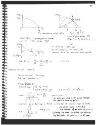
This first example will illustrate a turning point bifurcation for a one-dimensional<br />
system. Let the dynamics of the state w(t) described by the differential equation:<br />
dw<br />
dt = h(w, α) =w2 − α (3.1)<br />
The equilibrium solutions of this system satisfy the equation h(w, α) =0 =⇒ w 2 =<br />
α. This equation has no steady-state solutions for α0(w = √ α, w = − √ α). The Jacobian of h is<br />
∂h<br />
=2w. Since the system is one dimensional, the eigenvalue of the Jacobian is the<br />
∂w<br />
value of the Jacobian. For w0, the eigenvalue is positive, and so the equilibrium will<br />
be unstable. For w = 0, the eigenvalue is zero, and we encounter a turning point<br />
bifurcation. The following graph plots the steady-state solution branch as a function<br />
of the parameter α. Since for each value of α, the steady-state solution w(t) isa
CHAPTER 3. BIFURCATION ANALYSIS 47<br />
constant function, the plot shows what this constant value is as α changes. The<br />
Steady−State Solution (w)<br />
1<br />
0.8<br />
0.6<br />
0.4<br />
0.2<br />
0<br />
−0.2<br />
−0.4<br />
−0.6<br />
−0.8<br />
Unstable<br />
Stable<br />
Turning Point Bifurcation<br />
−1<br />
−1 −0.8 −0.6 −0.4 −0.2 0<br />
Parameter<br />
0.2 0.4 0.6 0.8 1<br />
Figure 3.1: Steady-State Solution Branch of dw<br />
dt = h(w, α) =w2 − α<br />
solution curve has a lower branch that is stable until the parameter α =0. The<br />
curve then reverses direction at the turning point (α, w) =(0, 0) and continues in the<br />
direction of increasing parameter α. Note that the stability of the solutions change<br />
along the curve at the turning point as well.<br />
The second example is of a pitchfork bifurcation. Consider the differential equation<br />
dw<br />
dt = h(w, α) =w3 − αw (3.2)
CHAPTER 3. BIFURCATION ANALYSIS 48<br />
The equilibrium solutions of this ODE satisfy w(w 2 − α) =0. Sow = 0 is a solution<br />
for all α and w = √ α, w = − √ α are additional solutions for α ≥ 0. The Jacobian<br />
is ∂h<br />
∂w =3w2− α. For the solution w = 0, the Jacobian is −α. So w = 0 is stable<br />
for α>0 and unstable for α
CHAPTER 3. BIFURCATION ANALYSIS 49<br />
ODE that describes the states w(t),v(t) by<br />
dw<br />
dt = αw − v − w(w2 + v 2 )<br />
dv<br />
dt = w + αv − v(w2 + v 2 )<br />
where α is a parameter. The origin, (w, v) =(0, 0), is an equilibrium to the system.<br />
The Jacobian of this system at the origin is given by<br />
⎛ ⎞<br />
⎜α<br />
−1⎟<br />
⎜ ⎟<br />
⎝ ⎠<br />
1 α<br />
and its eigenvalues are α ± i. Therefore, since the real part of the eigenvalues is α,<br />
when α0 the origin will be<br />
an unstable equilibrium. This means α = 0 is a bifurcation point in parameter space.<br />
It is easier visualize what is going on is this example if we change to polar coor-<br />
dinates (¯r, θ). The ODE is these coordinates is given by<br />
d¯r<br />
dt =¯r(α − ¯r2 )<br />
dθ<br />
dt =1<br />
Changing to these coordinates decouples the ODE. If α0, then for 0 < ¯r
CHAPTER 3. BIFURCATION ANALYSIS 50<br />
(α − ¯r 2 ) > 0 =⇒ d¯r<br />
> 0. So ¯r = 0 is an unstable equilibrium, since any small<br />
dt<br />
increase in ¯r will force ¯r to continue to move away from ¯r =0. Inthecaseofα>0,<br />
if ¯r > √ α, then by a similar argument, d¯r<br />
dt < 0. So if ¯r = 0,¯r approaches √ α for<br />
α>0. So we have a stable closed orbit in this case.<br />
If we start the parameter α as a negative value, then the origin is a stable equi-<br />
librium. As we increase the parameter, the origin remains stable until α becomes<br />
positive. Then the origin turns unstable and an oscillatory solution to the ODE<br />
appears. This is what is known as a Hopf bifurcation. As shown in this example,<br />
a Hopf bifurcation is characterized by a pair of complex-conjugate eigenvalues’ real<br />
parts going to zero.<br />
3.3 Continuation Methods<br />
Continuation algorithms map out a system’s steady-state solution branches as a sys-<br />
tem parameter is being changed. To do this numerically, we connected our simulator<br />
to the Library of Continuation Algorithms (LOCA), a software library developed at<br />
Sandia National Laboratories [33]. LOCA has three continuation algorithms available<br />
for the user: a zero order continuation, a first order continuation, and a pseudo arc-<br />
length continuation. LOCA also incorporates an eigensolver that checks the eigenval-<br />
ues of the Jacobian matrix of the system to determine the stability of the steady-state<br />
solution.<br />
Numerically, we plan on generating a sequence of parameters {V j } along with
CHAPTER 3. BIFURCATION ANALYSIS 51<br />
a corresponding sequence of steady-state solutions { f j } that satisfy W ( f j ,V j )=0.<br />
Since this is a nonlinear equation, Newton’s Method is used to calculate the steady-<br />
state solution f j for a specified V j . In a zero order continuation algorithm, the initial<br />
iterate used for Newton’s Method to compute f j+1 at V j+1 is f j .<br />
In the first order continuation algorithm, the sensitivity of the steady-state solu-<br />
tion to the parameter V is incorporated into the initial guess for the next Newton<br />
solve. The sensitivity of the previous steady-state solution f j to the parameter V ,<br />
given by ∂ f<br />
, is calculated by solving the linear system:<br />
∂V<br />
where the right hand side, ∂W<br />
∂V<br />
W ′ ( f j ) ∂ f<br />
∂V<br />
= ∂W<br />
∂V<br />
, is approximated by<br />
∂W<br />
∂V ≈ [W ( f j ,Vj + δ) − W ( f j ,Vj )]<br />
δ<br />
(3.3)<br />
(3.4)<br />
with δ being some small perturbation. Once V j+1 is determined, then the predictor<br />
used for the next Newton solve is f j + ∂ f<br />
∂V (V j+1 − V j ).<br />
Pseudo arc-length continuation [18] is used when continuing around turning points.<br />
As previously stated, when turning point bifurcations occur, the Jacobian matrix be-<br />
comes singular. So applying Newton’s method would become difficult as we approach<br />
the turning point since the Jacobian matrix is becoming singular, making the linear<br />
solves for the Newton steps harder. Pseudo arc-length continuation handles this prob-
CHAPTER 3. BIFURCATION ANALYSIS 52<br />
lem by augmenting the nonlinear equation W ( f,V) you are solving for steady-state<br />
with a contrived parameter s (the arc-length parameter) and an additional arc-length<br />
equation. So the system we are solving now is<br />
W ( f(s),V(s)) = 0 (3.5)<br />
N( f(s),V(s),s) = 0 (3.6)<br />
where the first equation specifies that we are on a steady-state solution branch, and<br />
the second equation specifies the step to take in the parameter s. Suppose we have<br />
the point ( f 0 ,V 0 ) on the solution curve and the next solution point to be computed<br />
is ( f j ,V j ). For the next continuation step, the arc-length equation is given by<br />
N( f(s),V(s),s)= ∂ T<br />
f<br />
(<br />
∂s<br />
f − f 0 )+ ∂V<br />
∂s (V − V 0 ) − ∆s (3.7)<br />
A geometric interpretation of the ( f,V)-points that satisfy N( f(s),V(s),s)=0can<br />
be given. Suppose a, b ∈ R and (x0,y0) ∈ R 2 . It is a result from analytic geometry<br />
that the points (x, y) ∈ R 2 where a(x − x0) +b(y − y0) − c = 0 lie in the plane<br />
perpendicular to the vector (a, b) atadistance<br />
√ c<br />
a2 +b2 away from (x0,y0). Similarly,<br />
if ( f j ,V j ) satisfy the arc length equation, then the point will lie in the ( f,V)plane<br />
perpendicular to the gradient of ( f(s),V(s)), at some distance away from ( f 0 ,V 0 ),<br />
determined by the size of ∆s. An example of tracing a one dimensional system with<br />
a one dimensional parameter using pseudo arc-length continuation is given in Figure
CHAPTER 3. BIFURCATION ANALYSIS 53<br />
3.3 below to further illustrate this point.<br />
Steady−state<br />
(f)<br />
Parameter (V)<br />
Current<br />
Point<br />
New<br />
Point<br />
Tangent<br />
Vector<br />
Newton (update)<br />
Step<br />
Figure 3.3: Illustration of Pseudo-Arc Length Continuation<br />
3.4 Linear Solver Methods for Pseudo Arc-Length<br />
Continuation<br />
When using natural continuation, the parameter V is fixed while an M dimensional<br />
nonlinear equation is solved for the state f. For pseudo arc-length continuation, the<br />
parameter V is also unknown, and the arc-length equation (3.7) must also be satisfied.<br />
This leads to the solution of M + 1 dimensional nonlinear equation, for both the M<br />
dimensional state f and the corresponding one dimensional parameter V . To solve
CHAPTER 3. BIFURCATION ANALYSIS 54<br />
the M + 1 dimensional nonlinear equation, we use Newton’s method. The combined<br />
M + 1 dimensional state of both the change in the steady-state, ∆ f, and the change<br />
in the parameter, ∆V , is the Newton step s ∈ R M+1 and is denoted by<br />
⎛<br />
⎞<br />
⎜∆<br />
s = ⎜<br />
⎝<br />
f ⎟<br />
⎠ ∈ RM+1<br />
∆V<br />
where f ∈ R M and V ∈ R. The M + 1 dimensional nonlinear equation to solve is<br />
given by ⎛<br />
⎜W<br />
(<br />
⎜<br />
⎝<br />
f,V)<br />
˜t T ⎞<br />
⎟<br />
⎠<br />
s − ∆s<br />
=<br />
⎛ ⎞<br />
⎜0⎟<br />
⎜ ⎟<br />
⎝ ⎠<br />
0<br />
∈ RM+1 .<br />
Here, W ( f,V) ∈ R M , s is defined as above, and ˜t ∈ R M+1 is the tangent vector of<br />
the steady-state solution curve with respect to the arc-length parameter s, i.e.<br />
⎛<br />
⎜<br />
˜t = ⎜<br />
⎝<br />
∂ f<br />
∂s<br />
∂V<br />
∂s<br />
⎞<br />
⎟<br />
⎠ ∈ RM+1 .<br />
The coefficient matrix for the linear system defining the Newton step s is given by<br />
⎛<br />
⎜<br />
⎝<br />
W ′ ( ∂W f) ∂V<br />
˜t T<br />
⎞<br />
⎟<br />
⎠ ∈ R(M+1)×(M+1)
CHAPTER 3. BIFURCATION ANALYSIS 55<br />
with right hand side ⎛<br />
⎜−W<br />
(<br />
⎜<br />
⎝<br />
⎞<br />
f,V) ⎟<br />
⎠<br />
∆s<br />
∈ RM+1 .<br />
In LOCA, there are two methods to solve this M + 1 dimensional linear system:<br />
bordering algorithms [33] or Householder continuation [37].<br />
3.5 Bordering Algorithms<br />
This method was motivated from the fact that while many application codes form<br />
and store the Jacobian matrix W ′ ( f), few create the M +1byM + 1 dimensional<br />
matrix needed for pseudo arc-length continuation. This method requires two linear<br />
solves per Newton iteration instead of the normal one linear solver per Newton itera-<br />
tion. The two solution vectors are then manipulated to create the M + 1 dimensional<br />
Newton step that satisfies (3.7). The bordering method is given by:<br />
• Solve W ′ ( f)y = −W and W ′ ( f)z = ∂W<br />
∂V<br />
• Parameter update: ∆V = −(N + ∂ T<br />
f<br />
y)/(<br />
∂s<br />
∂V<br />
∂s + ∂ T<br />
f<br />
z)<br />
∂s<br />
• Distribution update: ∆ f = y +∆Vz
CHAPTER 3. BIFURCATION ANALYSIS 56<br />
3.6 Householder Continuation<br />
This method based on [37] was implemented in LOCA. The idea is to create an embed-<br />
ding E : R M → R M+1 such that for each y ∈ R M , Ey2 = y2 and Ey is orthogonal<br />
to the subspace created by the span of ˜t. Householder projections achieve this in a<br />
computationally efficient fashion. Also, Ey satisfies the one dimensional constraint<br />
(3.7) automatically for all y ∈ R M , and thus the constraint (3.7) is automatically<br />
built into each Newton step. Let Q : RM+1 → RM be the matrix Q = W ′ (f) ∂W<br />
<br />
. ∂V<br />
This is the Jacobian matrix of W with respect to the both the state variable f and<br />
the parameter V . Now the composition QE is a linear operator that maps vectors<br />
in R M to vectors in R M . The idea is to solve the linear system QE˜s = −W ( f,V)<br />
for ˜s ∈ R M and call its embedding the Newton step s = E˜s. An algorithm of this<br />
method is as follows:<br />
• Compute embedding E given tangent vector ˜t<br />
• Use GMRES to solve QE˜s = −W ( f,V) for ˜s<br />
• Set the Newton step s to E˜s.<br />
This method requires only the construction of E (which can be done quickly), and one<br />
linear solve with the coefficient matrix of QE. Since the bordering algorithms require<br />
two linear solves, we expect a factor of two speed up from using the Householder<br />
continuation instead of the bordering algorithm. Further, the linear solves within the<br />
Householder continuation will be better conditioned than the linear solves within the
CHAPTER 3. BIFURCATION ANALYSIS 57<br />
bordering method. This is because the bordering method’s coefficient matrix is the<br />
Jacobian matrix W ′ ( f) which will be going singular at turning points.<br />
3.7 Parallelization of Simulator<br />
Since LOCA has been developed to run with both serial and parallel applications<br />
and adding grid points to enhance the accuracy of the simulation would substan-<br />
tially increase computational time, we were motivated to parallelize the simulator.<br />
Therefore, we had to determine how we would split apart the f vector and the W ( f)<br />
evaluation across the different processors. We decided to divide the f vector across<br />
the processors by the spatial variable x. This meant each processor had a contiguous<br />
block of x-space, with each processor owning all of the possible k values for each x<br />
grid point it had. This makes computing integrals in k-space a completely parallel<br />
process, with no communication between processors required, but the integral and<br />
derivative term in x-space will require communication between the processors. One<br />
could have done the opposite, where each processor gets a continugous block of k-<br />
space, with each processor owning all of the possible x values for each k grid point it<br />
had. In this case, computing the derivative and integral in x-space would be trivial<br />
while requiring communication between processors to compute the k-space integrals.<br />
We chose the way we distributed the data between the processors because there are<br />
more k-space integrals to compute, and they are the most computationally intensive<br />
part of the simulation.
CHAPTER 3. BIFURCATION ANALYSIS 58<br />
To handle the nonlinearity in computing W ( f), each processor computed the elec-<br />
tron density n(x) (1.11) for each x-point it owned. The processors would then send<br />
theirpartofn(x) to one processor, which is designated the main processor. This<br />
main processor takes all of n(x), performs the Poisson solve to compute the potential<br />
energy U(x) (1.13), and sends out U(x) to all the processors. Once each processor<br />
had U(x), it could compute P ( f) for each of its x-points. To compute the derivative<br />
term in K( f), each processor would need to know the f values on the 2 x grid points<br />
before its smallest x-point and the 2 x grid point ahead of its largest x-point since a<br />
second-order upwind differencing scheme was used. These values were passed between<br />
the processors. Finally, each processor would add these terms up to get the W ( f)<br />
evaluation on the parts of the domain the processor owned.<br />
To demonstrate the parallel efficiency of our program, the simulation with Nx =<br />
512 and Nk = 2048 was run using from 2 up to 80 processors. The runs reported<br />
in this section were performed on processors of a Linux cluster at Sandia National<br />
Laboratories. This cluster has a total of 236 compute nodes. The nodes are dual<br />
3.06 GHz Xeon processors, each with 2 GB of RAM. The table below compares the<br />
run times for taking 5 continuation steps, from V =0.2093 to V =0.2293. Since<br />
the nodes used to perform the efficiency study are dual processor, we decided a fair<br />
evaluation of the efficiency required a base case of 2 processors instead of the normal<br />
1 processor. The communication between 2 processors on the same node would be<br />
more efficient than the communication between processors across distinct nodes.
CHAPTER 3. BIFURCATION ANALYSIS 59<br />
Table 3.1: Computation of Parallel Efficiency<br />
#ofProcs. Linear Solve Time (s) Efficiency (Percent)<br />
2 9120.61 100 (Base case)<br />
4 4904.46 92.88<br />
8 3422.43 88.83<br />
12 1925.05 78.96<br />
16 1581.53 72.09<br />
24 1171.00 64.91<br />
32 966.06 59.01<br />
40 908.92 55.75<br />
48 771.91 53.34<br />
56 712.25 47.43<br />
64 667.62 42.69<br />
72 662.24 38.26<br />
80 641.39 35.55<br />
Amdahl’s Law [2] relates the percent of a code that is serial, the number of pro-<br />
cessors used, and the corresponding parallel efficieny for these processors. If ¯ N is the<br />
number of processors, Ē is the parallel efficiency, and ¯ S is the percent of the code<br />
that is serial, then Amdahl’s Law is<br />
Ē =<br />
1<br />
¯N ¯ S +(1− ¯ . (3.8)<br />
S)<br />
Therefore, Amdahl’s Law predicts an inverse relationship between the parallel effi-<br />
ciency of an application and the number of processors used when ¯ S = 0. Wecan<br />
use Amdahl’s Law and Table 3.1 to estimate the fraction of our application that is<br />
serial. This leads to a nonlinear least squares problem, where we fit our data with a<br />
theoretical curve that depends on one parameter ¯ S. To solve this problem, we used
CHAPTER 3. BIFURCATION ANALYSIS 60<br />
a nonlinear least squares code, available from [20], that uses a Levenberg-Marquardt<br />
algorithm to find the optimal value of ¯ S. This optimal value was computed to be<br />
¯S =0.0467. So Amdahl’s Law predicts that about 5 percent of our parallel code is<br />
actually in serial.<br />
Now we report on the scalability of the simulator. For the scalability results, we<br />
compared the performance of our simulator with a continuation run from V =0to<br />
V =0.33 for three different grids, each using a different number of processors. We<br />
start with a base case of Nx = 172, Nk = 144 and 2 processors, and then simultane-<br />
ously quadruple both the number of unknowns and the number of processors applied<br />
to the problem. We also want to emphasis that at the grids we are simulating, we<br />
do not have grid convergence. Therefore, we are not solving the same problem as<br />
the number of unknowns varies, and this must be considered when evaluating these<br />
results. Table 3.2 reports on the scalability of the simulator.<br />
Table 3.2: Scalability of RTD Simulation<br />
Nx Nk Run Time (min) No. of Cont. Steps Avg. W ( f) Evaluation Time (sec)<br />
172 144 30 34 0.0345<br />
344 288 51 34 0.0591<br />
688 576 112 38 0.1330<br />
Let n = Nx × Nk be the number of unknowns, and we will assume the serial and<br />
parallel work both scale as O(n β ), where β will be a parameter we fit from our data.<br />
If we let ¯ N be the number of processors, ¯ S be the serial fraction of our code, and scale
CHAPTER 3. BIFURCATION ANALYSIS 61<br />
the base time to be 1, then we can model the relative time T ∗ ( ¯ N) for the scalability<br />
runs as<br />
T ∗ ( ¯ N)= ¯ S ¯ N β +(1− ¯ S) ¯ N β−1<br />
which we can then use to get an estimate of the serial fraction of our code from the<br />
scalability data.<br />
From the scalability data, we have two data points (since the base case will be<br />
scaled to T ∗ = 1 and for all possible parameter values, the model has T ∗ (1) = 1).<br />
Since we have two data points and two parameters to fit, the parameter estimation<br />
is a solution to a nonlinear equation instead of a nonlinear least squares problem.<br />
Therefore, we used a Newton code from [19] to solve the two-dimensional problem.<br />
We did two separate nonlinear solves with this code, using in one case the total run<br />
times and in the second case using the average function evaluation times. For the<br />
total run time case, the values of ¯ S and β were ¯ S =4.33 percent and β =1.2948.<br />
The values of ¯ S and β were ¯ S =4.78 percent and β =1.2915 in the average function<br />
evaluation time case.<br />
From both the parallel efficiency and scalability results, we estimate that about 5<br />
percent of our parallel code is serial. The 5 percent serial code would be troublesome<br />
if we were to scale this problem to thousands of processors, but we do not need such<br />
a large-scale computing environment for the number of unknowns we are solving, and<br />
the 5 percent serial code does not hurt us that much on tens of processors.
CHAPTER 3. BIFURCATION ANALYSIS 62<br />
3.8 Linear Solver Comparison for Pseudo Arc-Length<br />
Continuation<br />
On the Nx = 512 and Nk = 2048 grid, we numerically compared the efficiency of<br />
the two methods for solving the linear system in pseudo arc-length continuation (as<br />
explain in Sections 3.4-3.6). We compared the methods by starting the continuation at<br />
a point on the solution curve and letting the method complete 7 steps in continuation.<br />
They followed the same path, and this path included turning points. The current-<br />
voltage plot is shown for this grid in Figure 3.4. Figure 3.5 shows an enlarged part<br />
of Figure 3.4 where the methods were compared.<br />
Current Density (10 5 A/cm 2 )<br />
6<br />
5<br />
4<br />
3<br />
2<br />
1<br />
0<br />
−1<br />
0 0.05 0.1 0.15 0.2 0.25 0.3 0.35 0.4 0.45<br />
Voltage Difference (V)<br />
Figure 3.4: Current-Voltage Plot<br />
Table 3.3 shows the number of total number of linear (GMRES) iterations, total
CHAPTER 3. BIFURCATION ANALYSIS 63<br />
Current Density (10 5 A/cm 2 )<br />
4.6<br />
4.5<br />
4.4<br />
4.3<br />
4.2<br />
4.1<br />
4<br />
3.9<br />
3.8<br />
3.7<br />
3.6<br />
0.23 0.232 0.234 0.236<br />
Voltage Difference (V)<br />
0.238 0.24 0.242<br />
Figure 3.5: Enlarged Portion of Curve Where Methods Were Compared<br />
number of nonlinear (Newton) iterations, and total time to take 7 pseudo arc-length<br />
continuation steps.<br />
Table 3.3: Comparison of Bordering and Householder Methods<br />
Method No. of GMRES Its. No. of Newton Its. Solution Time (sec)<br />
Bordering 8826 21 5905<br />
Householder 3026 15 2016<br />
We previously expected a factor of 2 savings from using Householder continuation<br />
instead of the bordering algorithm. The run times show a factor of 3 savings. An<br />
explanation of this is that, as previously stated, the Householder continuation linear<br />
solves were better conditioned than those of the bordering method. This is why
CHAPTER 3. BIFURCATION ANALYSIS 64<br />
GMRES was able to more efficiently solve the linear systems in the Householder<br />
continuation than in the bordering method.<br />
3.9 Results<br />
Once the simulator was connected with LOCA, the first thing we wanted to do was<br />
analyze the original grid Nx = 86, Nk = 72 that our project’s physicists and engi-<br />
neers had used in reporting results to the scientific community. These results [8],<br />
[40] reported hystersis in the current-voltage (I-V) curves and current oscillation for<br />
some values of applied bias. Figure 3.6 shows a forward sweep in bias from V =0to<br />
V =0.480, with increments of 0.08 taken in bias. As you can see, the I-V curve drops<br />
suddenly at 0.318 volts to a lower curve and continues on. In the reverse bias case,<br />
wherewestartatV =0.480 and reduce by 0.08 volts to V = 0, the I-V curve follows<br />
out this lower branch, but does not jump up at 0.318 volts. Instead, it continues along<br />
this lower curve, until it jumps back up to the upper curve at 0.256 volts. Figure 3.7<br />
shows the window of voltage that creates current oscillation within the device. We<br />
can see the oscillation onsets between 0.240 volts and 0.248 volts and turns off again<br />
between 0.256 volts and 0.264 volts.<br />
Using LOCA’s pseudo arc-length continuation algorithm and eigensolver, we were<br />
able to explain why these phenomena occur. Figure 3.8 shows the I-V curve generated<br />
by LOCA. LOCA has found two turning points: one at 0.256 volts and one at 0.318<br />
volts. The branch connecting the two is an unstable steady-state solution branch,
CHAPTER 3. BIFURCATION ANALYSIS 65<br />
Average Current Density (A/cm 2 )<br />
Current Density (A/cm 2 )<br />
7<br />
6<br />
5<br />
4<br />
3<br />
2<br />
1<br />
x 10 5 nx=86, nk=72 Grid: Time Integrator I−V Curve<br />
0<br />
0 0.05 0.1 0.15 0.2 0.25 0.3 0.35 0.4 0.45<br />
Applied Voltage (V)<br />
6.5<br />
6<br />
5.5<br />
5<br />
4.5<br />
4<br />
3.5<br />
x 105<br />
7<br />
Figure 3.6: I-V Curve Generated by Time-Accurate Simulation<br />
nx=86, nk=72 Grid<br />
0.240 V<br />
0.248 V<br />
0.256 V<br />
0.264 V<br />
3<br />
0 200 400 600 800 1000<br />
Time (fs)<br />
1200 1400 1600 1800 2000<br />
Figure 3.7: Bias Window of Current Oscillation
CHAPTER 3. BIFURCATION ANALYSIS 66<br />
Current Density (A/cm 2 )<br />
7<br />
6<br />
5<br />
4<br />
3<br />
2<br />
1<br />
x 10 5 nx=86, nk=72 Grid: LOCA I−V Curve<br />
0<br />
0 0.05 0.1 0.15 0.2 0.25 0.3 0.35 0.4 0.45<br />
Applied Voltage (V)<br />
Figure 3.8: I-V Curve Generated by LOCA<br />
which would not be detected by the time-accurate methods used by the engineers.<br />
This explains the hysteric effects we are seeing, since if the initial voltage is high, the<br />
solution can stay on a stable lower branch until 0.256 volts and if the initial voltage<br />
is low, the solution will stay on the higher stable branch until 0.318 volts.<br />
Figure 3.9 plots a pair of complex-conjugate eigenvalues of the Jacobian matrix<br />
as a function of volts, produced by LOCA’s eigensolver. As the plot shows, the eigen-<br />
values’ real parts go to zero between 0.240 volts and 0.2405 volts and stay positive<br />
until 0.256 volts. This explains why we are seeing the oscillation in the above bias<br />
window.<br />
As the grids were further refined, we were able to obtain grid convergence for the
CHAPTER 3. BIFURCATION ANALYSIS 67<br />
Imaginary Part<br />
0.02<br />
0.015<br />
0.01<br />
0.005<br />
0<br />
−0.005<br />
−0.01<br />
−0.015<br />
0.240<br />
0.242<br />
0.244<br />
0.246<br />
0.248<br />
0.250<br />
0.252<br />
0.254<br />
0.256<br />
Bifurcating Eigenvalues on nx=86,nk=72 Grid<br />
−5 −4 −3 −2 −1 0 1 2<br />
x 10 −3<br />
−0.02<br />
Real Part<br />
Figure 3.9: Eigenvalues Creating Oscillatory Solutions<br />
current-voltage plots. Figure 3.10 compares the previous grid results for Nx = 86,<br />
Nk = 72 (about 6,000 unknowns) to the results for the grids Nx = 512, Nk = 2048<br />
(about 1 million unknowns) and Nx = 1024, Nk = 2048 (about 2 million unknowns).<br />
The current-voltage plots of the 1 million unknown and 2 million unknown grids lie<br />
on top of one another. These grids present new physics in the current voltage-plot as<br />
previously shown from the coarser grid. The plot in general is shifted down, having<br />
a smaller global maximum than the coarser grid plot. There are more local minima<br />
and maxima in the refined grid plots as well.
CHAPTER 3. BIFURCATION ANALYSIS 68<br />
Current Density (A/cm 2 )<br />
x Grid 105<br />
7<br />
6<br />
5<br />
4<br />
3<br />
2<br />
1<br />
0<br />
Refinement<br />
nx=512, nk=2048<br />
nx=1024, nk=2048<br />
nx=86, nk=72<br />
−1<br />
0 0.05 0.1 0.15 0.2 0.25 0.3 0.35 0.4 0.45 0.5<br />
Applied Voltage (V)<br />
Figure 3.10: Comparison of Current-Voltage Plots for Varying Grids<br />
3.10 Correlation Length Study<br />
3.10.1 Current Voltage Relationship<br />
The current-voltage (I-V) curve generated by the fine mesh simulation looked un-<br />
physical when evaluated by the physicists in our research group. As shown in Figure<br />
3.10, the fine mesh I-V curve has several peaks, and the physicists do not expect<br />
these. In the original coarse grid simulation (Nx = 86, Nk = 72), the correlation<br />
length was varied until the simulation produced a physical I-V curve. Since we have<br />
refined the mesh, the correlation length needs to be changed again so that the I-V<br />
curve agrees with what physicists believe to be correct. Figures 3.11-3.15 show sev-
CHAPTER 3. BIFURCATION ANALYSIS 69<br />
Current Density (A/cm 2 )<br />
x 105<br />
7<br />
6<br />
5<br />
4<br />
3<br />
2<br />
1<br />
0<br />
0 0.05 0.1 0.15 0.2<br />
Applied Voltage (V)<br />
0.25 0.3 0.35 0.4<br />
Figure 3.11: I-V Curve with 30 Percent Reduced Correlation Length<br />
erla I-V curves where correlation length has been change. Figues 3.11-3.13 involved<br />
a reduced correlation length from the original simulation, and Figures 3.14 and 3.15<br />
involve and increased correlation length. The increased correlation length simulations<br />
produce I-V curves that have even more peaks than the original correlation length<br />
simulations. The reduced correlation length simulations produce more realistic I-V<br />
curves, with the 20 percent reduced correlation length creating the most favorable<br />
I-V curve when evaluated by the physicists.
CHAPTER 3. BIFURCATION ANALYSIS 70<br />
Current Density (A/cm 2 )<br />
Current Density (A/cm 2 )<br />
x 105<br />
7<br />
6<br />
5<br />
4<br />
3<br />
2<br />
1<br />
0<br />
0 0.05 0.1 0.15 0.2<br />
Applied Voltage (V)<br />
0.25 0.3 0.35 0.4<br />
x 105<br />
7<br />
6<br />
5<br />
4<br />
3<br />
2<br />
1<br />
Figure 3.12: I-V Curve with 25 Percent Reduced Correlation Length<br />
0<br />
0 0.05 0.1 0.15 0.2<br />
Applied Voltage (V)<br />
0.25 0.3 0.35 0.4<br />
Figure 3.13: I-V Curve with 20 Percent Reduced Correlation Length
CHAPTER 3. BIFURCATION ANALYSIS 71<br />
Current Density (A/cm 2 )<br />
Current Density (A/cm 2 )<br />
x 105<br />
7<br />
6<br />
5<br />
4<br />
3<br />
2<br />
1<br />
0<br />
0 0.05 0.1 0.15 0.2<br />
Applied Voltage (V)<br />
0.25 0.3 0.35 0.4<br />
x 105<br />
7<br />
6<br />
5<br />
4<br />
3<br />
2<br />
1<br />
Figure 3.14: I-V Curve with 10 Percent Increased Correlation Length<br />
0<br />
0 0.05 0.1 0.15 0.2 0.25 0.3 0.35 0.4<br />
Figure 3.15: I-V Curve with 20 Percent Increased Correlation Length
CHAPTER 3. BIFURCATION ANALYSIS 72<br />
3.10.2 Stability Analysis<br />
We performed a stability analysis on the steady state electron distribution for the<br />
20 percent reduced correlation length. This enabled us to test out the performance<br />
of the Cayley transformation on these large scale matrices where iterative solvers<br />
are used to solve the linear systems. The Cayley transformation (as explained in<br />
Appendix B) is a way to transform the standard eigenvalue problem to one where<br />
unstable eigenvalues of the Jacobian will be detected first. We were checking the<br />
I-V curves for voltage values where we expect current oscillations. From the the<br />
coarse grid simulations, the current oscillations occured after the I-V curve was at<br />
its maximum value, where the current ouput decreases as the applied voltage drop<br />
was increased. This phenomenon is known as negative differential resistance, and<br />
we checked similar areas on the fine grid I-V curve for current oscillation. Table<br />
3.4 lists the voltage values where we checked for current oscillation. The table lists<br />
the converged eigenvalue as well as the Rayleigh quotient residual for the eigenvalue,<br />
which is a measure of how accurate the eigenvalue is. Appendix D explains more<br />
on the algorithm used to compute the eigenvalues (the Arnoldi method) as well as<br />
explaining the Rayleigh quotient residual. These computations were performed on 20<br />
processors of a Linux cluster maintained by the High Performance Computing center<br />
at North Carolina State University. The average time for an Arnoldi iteration was 740<br />
seconds. This means that it took approximately 40 hours to converge one eigenvalue<br />
of the Jacobian matrix at one voltage value. The closest we came to finding current
CHAPTER 3. BIFURCATION ANALYSIS 73<br />
oscillation was at V =0.27. Here, the real part of the eigenvalue is two orders of<br />
magnitude smaller than the imaginary part. The size of the imaginary part also<br />
corresponds to a THz frequency oscillation. While the I-V curve generated by the<br />
20 percent reduced correlation length was the most favorable with the physicists, the<br />
stability analysis of the I-V curve did not generate a voltage value where we expect<br />
current oscillation.<br />
Table 3.4: Eigenvalue Calculations for 20 Percent Reduced Correlation Length<br />
Voltage Eigenvalue Rayleigh Quotient Residual<br />
0.251 -9.686e-04 - 9.108e-04 i 6.153e-09 + 2.168e-08 i<br />
0.269 -4.502e-04 - 1.809e-02 i 5.625e-06 + 4.962e-06 i<br />
0.27 -4.820e-04 + 1.828e-02 i 4.704e-06 + 4.373e-06 i<br />
0.27083 -6.199e-04 - 1.847e-02 i 5.922e-06 + 4.644e-06 i<br />
0.28 -1.705e-03 - 6.555e-04 i 5.207e-10 + 4.105e-10 i<br />
0.288 -1.704e-03 - 6.947e-04 i 2.901e-09 + 7.396e-09 i<br />
0.2977 -1.686e-03 - 7.439e-04 i 1.273e-09 + 5.428e-09 i<br />
0.30 -1.681e-03 + 7.613e-04 i 5.474e-09 + 3.180e-08 i<br />
0.304 -1.681e-03 - 8.077e-04 i 7.746e-09 + 1.185e-08 i<br />
0.312 -1.452e-03 - 1.387e-03 i 2.870e-09 + 5.092e-09 i<br />
0.3157 -1.095e-03 + 9.444e-04 i 5.079e-09 + 2.618e-08 i
Chapter 4<br />
Theory<br />
4.1 Steady-State Theory<br />
In this chapter, we are concerned with theoretically analyzing the infinite-dimensional<br />
steady-state solutions of the Wigner-Poisson equations as the applied voltage drop<br />
V > 0 is varied. We will recast the problem as a fixed point problem of the form<br />
f(x, k) =Z(f)(x, k)+ā(x, k), where the steady-state solutions of the Wigner-Poisson<br />
equations are the fixed points of this map. We will analyze this fixed point map in<br />
the function space<br />
with norm<br />
Kmax<br />
X = {u(x, k)|<br />
−Kmax<br />
|u(x, k ′ )| 2 dk ′ ∈ C [0,L]}<br />
Kmax<br />
uX = max |u(x, k<br />
x∈[0,L] −Kmax<br />
′ )| 2 dk ′<br />
1<br />
2<br />
.<br />
74
CHAPTER 4. THEORY 75<br />
Theideaisto<br />
1. Show Z maps X to X.<br />
2. Show Z is continuous on X.<br />
3. Show Z is a compact operator on X.<br />
WecanthenusethefactthatZ is a compact operator to show that its Frechet<br />
derivative, denoted by Z ′ , is a compact linear operator from X to X. This will allow<br />
us to show that when the iterative linear solver GMRES is applied to the infinite-<br />
dimensional problem, the norms of the residuals quickly converges to zero as the<br />
iteration continues, which helps to explain the mesh-independence performance we see<br />
in the finite-dimensional numerical approximation to the Wigner-Poisson equations.<br />
At the very end of the chapter, we also attempt to use the compactness of Z with the<br />
Schauder Fixed Point theorem to prove the existence of steady-state solutions and<br />
show how a simple application of this theorem does not immediately work.<br />
Rewrite Steady-State Solutions as Fixed Points<br />
The steady-state solutions will satisfy the nonlinear equation<br />
W (f) =K(f)+P (f)+S(f) =0.
CHAPTER 4. THEORY 76<br />
If we write out and rearrange the terms, set the constant C = 2πm∗<br />
hτ , assume k = 0,<br />
then we have<br />
∂f<br />
∂x +C<br />
k<br />
f(x, k) =C<br />
k<br />
If we note that<br />
f0(x, k)<br />
Kmax<br />
−Kmax f0(x, k ′ )dk ′<br />
∂<br />
<br />
∂x<br />
f(x, k)e Cx<br />
k<br />
<br />
Kmax<br />
−Kmax<br />
= ∂f Cx<br />
e<br />
∂x<br />
then by multiplying each side by e Cx<br />
k ,wehave<br />
∂<br />
<br />
∂x<br />
f(x, k)e Cx<br />
k<br />
<br />
= C<br />
k<br />
We will now consider two cases:<br />
Case 1: k>0<br />
f(x, k ′ )dk ′ − 4Cτ<br />
hk<br />
k + C<br />
k<br />
f(x, k)e Cx<br />
k ,<br />
f0(x, k)e Cx<br />
k<br />
Kmax<br />
−Kmax f0(x, k ′ )dk ′<br />
Kmax<br />
f(x, k<br />
−Kmax<br />
′ )dk ′ − 4Cτ<br />
hk<br />
Kmax<br />
−Kmax<br />
Kmax<br />
−Kmax<br />
f(x, k ′ )T (x, k−k ′ )dk ′ .<br />
When k>0, we have boundary conditions for f(x, k)atx =0,thatisf(0,k)=f1(k).<br />
So, we have<br />
f(x, k)e Cx<br />
k − f(0,k)=<br />
x<br />
Therefore, we can integrate from 0 to x to get:<br />
0<br />
dz ∂<br />
<br />
∂z<br />
f(z,k)e Cz<br />
k<br />
Cx<br />
−<br />
f(x, k) =e k f1(k)+G1(f)+G2(f)<br />
<br />
.<br />
e Cx<br />
k f(x, k ′ )T (x, k−k ′ )dk ′ .
CHAPTER 4. THEORY 77<br />
where we will define G1(f) andG2(f) shortly.<br />
Case 2: k
CHAPTER 4. THEORY 78<br />
So if we write Z(f) =G1(f)+G2(f) andsetā(x, k) as<br />
⎧<br />
Cx ⎪⎨ − e k f1(k), if k>0<br />
ā(x, k) =<br />
⎪⎩ e C(L−x)<br />
k f2(k), if k
CHAPTER 4. THEORY 79<br />
given by<br />
Kmax<br />
−Kmax<br />
|u(x, k ′ )|dk ′ =<br />
≤<br />
Kmax<br />
−Kmax<br />
Kmax<br />
−Kmax<br />
(1)|u(x, k ′ )|dk ′<br />
≤ 2KmaxuX.<br />
1 2 dk ′<br />
1<br />
2 Kmax<br />
−Kmax<br />
|u(x, k ′ )| 2 dk ′<br />
1<br />
2<br />
We will now get an estimate for T (x, k − k ′ ) for u ∈ L 2 ([0,L] × [−Kmax,Kmax]). By<br />
Equation (1.16), we know that U(x) is the sum of the electrostatic potential up(x)and<br />
the potential barriers ∆c(x). The dependence of T (x, k −k ′ )onu is through Poisson’s<br />
equation (Equation (1.13)). We can solve Poisson’s equation explicitly through the<br />
use of a Green’s function [13]. The Green’s function for Poisson’s equation in one<br />
dimension for the domain [0,L]isgivenby<br />
Therefore, the exact solution up(x) isgivenby<br />
L<br />
up(x) =<br />
0<br />
⎧<br />
⎪⎨ z(<br />
J(x, z) =<br />
⎪⎩<br />
x − 1), if 0 ≤ z ≤ x<br />
L<br />
x( z<br />
. (4.4)<br />
− 1), if x ≤ z ≤ L<br />
L<br />
2 q<br />
J(x, z) Nd(z) −<br />
ɛ<br />
1<br />
Kmax<br />
u(z,k<br />
2π −Kmax<br />
′ )dk ′<br />
<br />
dz.
CHAPTER 4. THEORY 80<br />
Combining Equation 1.16 for U(x) and Equation 1.9 for T (x, z), we get that the<br />
explicit dependence of T (x, k − k ′ )onu is given by<br />
T (x, k − k ′ )= q2<br />
Lc<br />
2<br />
2πɛ 0<br />
L Kmax<br />
0<br />
[J(x − y, z) − J(x + y, z)] sin(2y(k − k<br />
−Kmax<br />
′ ))u(z,k ′′ )dk ′′ dzdy<br />
Lc L 2<br />
+ q2<br />
ɛ<br />
0<br />
+<br />
0<br />
Lc<br />
2<br />
0<br />
[J(x + y, z) − J(x − y, z)] sin(2y(k − k ′ ))Nd(z)dzdy<br />
dy sin(2y(k − k ′ <br />
)) ∆c(x + y) − ∆c(x − y) − 2Vy<br />
<br />
.<br />
L<br />
We note that T (x, k − k ′ ) is a continuous function. To get an upper bound on<br />
||T ||∞, we will look at each term of T (x, k − k ′ ) individually. Define T1(x, k − k ′ )as<br />
T1(x, k−k ′ )= q2<br />
Lc<br />
2<br />
2πɛ 0<br />
So,<br />
<br />
<br />
|T1(x, k − k)| = q2<br />
2πɛ<br />
≤ q2<br />
2πɛ<br />
L Kmax<br />
Lc<br />
2<br />
0<br />
Lc<br />
2<br />
0<br />
0<br />
≤ q2<br />
2πɛ<br />
−Kmax<br />
[J(x−y, z)−J(x+y, z)] sin(2y(k−k ′ ))u(z,k ′′ )dk ′′ dzdy.<br />
L Kmax<br />
0 −Kmax [J(x − y, z) − J(x + y, z)] sin(2y(k − k′ ))u(z,k ′′ )dk ′′ dzdy<br />
L Kmax<br />
0 −Kmax |[J(x − y, z) − J(x + y, z)] sin(2y(k − k′ ))u(z,k ′′ )|dk ′′ dzdy<br />
Lc<br />
2<br />
0<br />
≤ q2<br />
2πɛ<br />
Lc<br />
2<br />
0<br />
L Kmax<br />
0 −Kmax 2||J||∞|u(z,k ′′ )|dk ′′ dzdy<br />
L Kmax<br />
0 −Kmax 4||J||2∞dk ′′ dz<br />
1<br />
2 L<br />
0<br />
= q2Lc 4πɛ 2J∞<br />
√<br />
2KmaxLu2.<br />
Kmax<br />
−Kmax u2 (z,k ′′ )dk ′′ 1<br />
2<br />
dz
CHAPTER 4. THEORY 81<br />
By definition of J(x, z) in Equation (4.4), then ||J||∞ = L.<br />
Therefore,<br />
4<br />
|T1(x, k − k)| ≤ q2 Lc<br />
8πɛ L 2KmaxLu2.<br />
When bounding the second term, T2(x, k − k ′ ), we get<br />
|T2(x, k − k ′ )| =<br />
<br />
<br />
q2<br />
ɛ<br />
≤ q2<br />
ɛ<br />
≤ q2<br />
ɛ<br />
Lc<br />
2<br />
0<br />
Lc<br />
2<br />
0<br />
Lc<br />
2<br />
0<br />
≤ q2<br />
4ɛ LcL 2 ||Nd||∞.<br />
L<br />
[J(x + y, z) − J(x − y, z)] sin(2y(k − k ′ <br />
<br />
))Nd(z)dzdy<br />
0<br />
L<br />
|[J(x + y, z) − J(x − y, z)] sin(2y(k − k ′ ))Nd(z)|dzdy<br />
0<br />
L<br />
2||J||∞||Nd||∞dzdy<br />
The third term, T3(x, k − k ′ ), is bound by<br />
|T3(x, k − k ′ )| =<br />
≤<br />
≤<br />
<br />
<br />
<br />
Therefore, we have that<br />
Lc<br />
2<br />
0<br />
Lc<br />
2<br />
0<br />
Lc<br />
2<br />
0<br />
0<br />
dy sin(2y(k − k ′ <br />
)) ∆c(x + y) − ∆c(x − y) − 2Vy<br />
<br />
<br />
<br />
dy<br />
sin(2y(k − k ′ <br />
)) ∆c(x + y) − ∆c(x − y) − 2Vy<br />
<br />
L<br />
dy[2||∆c||∞ + 2Vy<br />
L ]<br />
= ||∆c||∞Lc + VL2 c<br />
4L .<br />
||T ||∞ ≤ q2 Lc<br />
8πɛ L 2KmaxLu2 + q2<br />
4ɛ LcL 2 ||Nd||∞ + ||∆c||∞Lc + VL2 c<br />
4L .<br />
L
CHAPTER 4. THEORY 82<br />
We now estimate |G1(u)(x, k)|. Let ¯ h(x, k) =<br />
f0(x,k)<br />
Kmax<br />
−Kmax f0(x,k ′ . Our assumptions on<br />
)dk ′<br />
f0(x, k) imply ¯ h ∈ L ∞ ([0,L] × [−Kmax,Kmax]). For k>0wehave<br />
|G1(u)(x, k)| =<br />
and for k
CHAPTER 4. THEORY 83<br />
dent of x, wehaveG1(u)X ≤ 2Kmax ¯ h∞uX.<br />
For an estimate of |G2(u)(x, k)|, we have for k>0<br />
and k
CHAPTER 4. THEORY 84<br />
pendent of x, wehaveG2(u)X ≤ 8τKmax T ∞uX.<br />
h<br />
We now want to show that Kmax<br />
−Kmax |G1(u)(x, k ′ )| 2 dk ′ ∈ C[0,L]and Kmax<br />
−Kmax |G2(u)(x, k ′ )| 2 dk ′ ∈<br />
C[0,L]. Let x, y ∈ [0,L]. Fix γ>0. We want to show that Kmax<br />
−Kmax G1(u)(x, k ′ ) 2 dk ′<br />
is continuous. So<br />
Kmax<br />
<br />
G1(u)(x, k)<br />
−Kmax<br />
2 Kmax<br />
dk − G1(u)(y, k)<br />
−Kmax<br />
2 Kmax<br />
<br />
dk<br />
= [G1(u)(x, k)<br />
−Kmax<br />
2 − G1(u)(y, k) 2 <br />
<br />
]dk<br />
Kmax<br />
<br />
<br />
<br />
= [G1(u)(x, k) − G1(u)(y, k)][G1(u)(x, k)+G1(u)(y, k)]dk<br />
−Kmax<br />
Kmax<br />
≤ |G1(u)(x, k) − G1(u)(y, k)|[|G1(u)(x, k)| + |G1(u)(y, k)|]dk<br />
−Kmax<br />
≤ 8KmaxuX¯ Kmax<br />
h∞ |G1(u)(x, k) − G1(u)(y, k)|dk.<br />
−Kmax<br />
So an estimate of Kmax<br />
−Kmax |G1(u)(x, k ′ ) 2 − G1(u)(y, k ′ ) 2 |dk ′ is bounded by an estimate<br />
of Kmax<br />
−Kmax |G1(u)(x, k) − G1(u)(y, k)|dk. We will consider this integral first on the<br />
interval (0,Kmax]. Here, we have<br />
Kmax<br />
Kmax <br />
<br />
|G1(u)(x, k) − G1(u)(y, k)|dk = <br />
0<br />
0<br />
C<br />
x<br />
k 0<br />
y<br />
− C<br />
k<br />
0<br />
dz¯ h(z,k)e C(z−x)<br />
k<br />
dz¯ h(z,k)e C(z−y)<br />
k<br />
Kmax<br />
Kmax<br />
−Kmax<br />
−Kmax<br />
u(z,k ′ )dk ′<br />
u(z,k ′ )dk ′<br />
<br />
<br />
dk.
CHAPTER 4. THEORY 85<br />
Without loss of generality, assume y 0. Then the two intervals are (0,ɛk) and[ɛk,Kmax]. For the first<br />
<br />
dk
CHAPTER 4. THEORY 86<br />
interval we have:<br />
<br />
2Kmax¯ ɛk <br />
h∞uX 2 − 2e<br />
0<br />
C(y−x)<br />
k + e −Cx<br />
k − e −Cy<br />
k dk<br />
≤ 2Kmax¯ ɛk<br />
h∞uX |2 − 2e<br />
0<br />
C(y−x)<br />
k + e −Cx<br />
k − e −Cy<br />
k |dk<br />
≤ 2Kmax¯ ɛk <br />
h∞uX 2+2e<br />
0<br />
C(y−x)<br />
k + e −Cx<br />
k + e −Cy<br />
k dk<br />
≤ 2Kmax¯ ɛk<br />
h∞uX [2+2+1+1]dk<br />
0<br />
=6 2Kmax ¯ h∞uXɛk.<br />
We want to choose ɛk so that the bound over this first interval is equal to γ<br />
4 .Onthe<br />
second interval we have:<br />
<br />
2Kmax¯ Kmax<br />
h∞uX<br />
ɛk<br />
≤ 2Kmax¯ Kmax<br />
h∞uX<br />
ɛk<br />
≤ 3 2Kmax¯ Kmax<br />
h∞uX<br />
<br />
2 − 2e C(y−x)<br />
k + e −Cx<br />
k − e −Cy<br />
k dk<br />
|2 − 2e C(y−x)<br />
ɛ k | + e −Cy<br />
k |e C(y−x)<br />
ɛ k − 1|dk<br />
|1 − e C(y−x)<br />
ɛ k |dk<br />
ɛk<br />
=3 2Kmax¯ h∞uX(Kmax − ɛk)|1 − e C(y−x)<br />
ɛk |<br />
≤ 3Kmax<br />
2Kmax ¯ h∞uX|1 − e C(y−x)<br />
ɛ k |.<br />
We want to choose x and y close enough together so that this bound over the second<br />
interval is equal to γ<br />
Cx<br />
ɛ . We can do this since e k is a continuous function. Therefore,<br />
4
CHAPTER 4. THEORY 87<br />
we have shown that we can choose x and y close enough so that<br />
Kmax<br />
0<br />
|G1(u)(x, k) 2 − G1(u)(y, k) 2 |dk ≤ γ<br />
2 .<br />
Using a very similar argument for the case k0. We want to show that Kmax<br />
−Kmax G2(u)(x, k ′ ) 2 dk ′ is<br />
continuous. So<br />
Kmax<br />
<br />
G2(u)(x, k)<br />
−Kmax<br />
2 Kmax<br />
dk − G2(u)(y, k)<br />
−Kmax<br />
2 Kmax<br />
<br />
dk<br />
= [G2(u)(x, k)<br />
−Kmax<br />
2 − G2(u)(y, k) 2 <br />
<br />
]dk<br />
Kmax<br />
<br />
<br />
<br />
= [G2(u)(x, k) − G2(u)(y, k)][G2(u)(x, k)+G2(u)(y, k)]dk<br />
−Kmax<br />
Kmax<br />
≤ |G2(u)(x, k) − G2(u)(y, k)|[|G2(u)(x, k)| + |G2(u)(y, k)|]dk<br />
−Kmax<br />
≤ 8τ<br />
h<br />
<br />
Kmax<br />
2KmaxuXT ∞ |G2(u)(x, k) − G2(u)(y, k)|dk.<br />
−Kmax
CHAPTER 4. THEORY 88<br />
So an estimate of Kmax<br />
−Kmax |G2(u)(x, k ′ ) 2 − G2(u)(y, k ′ ) 2 |dk ′ is bounded by an estimate<br />
of Kmax<br />
−Kmax |G2(u)(x, k) − G2(u)(y, k)|dk. We will first consider this integral on the<br />
interval (0,Kmax]. Next, we have<br />
Kmax<br />
Kmax <br />
<br />
|G2(u)(x, k) − G2(u)(y, k)|dk = <br />
0<br />
0<br />
4Cτ<br />
y<br />
hk 0<br />
x<br />
− 4Cτ<br />
hk<br />
0<br />
dze C(z−y)<br />
k<br />
dze C(z−x)<br />
k<br />
Kmax<br />
Kmax<br />
−Kmax<br />
Without loss of generality, assume y
CHAPTER 4. THEORY 89<br />
So, we have<br />
Kmax<br />
|G2(u)(x, k) − G2(u)(y, k)|dk<br />
0<br />
<br />
e −Cx<br />
x<br />
C Cz<br />
k e k dz +<br />
y k C −Cy<br />
[e k − e<br />
k −Cx<br />
y<br />
k ] e<br />
0<br />
Cz<br />
<br />
k dz dk<br />
= 4τ <br />
Kmax <br />
2KmaxT ∞uX 1 − e<br />
h<br />
0<br />
C(y−x) <br />
k + e −Cy<br />
k − e −Cx<br />
<br />
k e Cy <br />
k − 1 dk<br />
= 4τ <br />
Kmax <br />
2KmaxT ∞uX 1 − e<br />
h<br />
0<br />
C(y−x) <br />
k + 1 − e C(y−x)<br />
k − e −Cy<br />
k + e −Cx<br />
<br />
k dk<br />
= 4τ <br />
Kmax <br />
2KmaxT ∞uX 2 − 2e<br />
h<br />
C(y−x)<br />
k + e −Cx<br />
k − e −Cy<br />
k dk.<br />
≤ 4τ <br />
Kmax<br />
2KmaxT ∞uX<br />
h<br />
0<br />
We will now break the k interval (0,Kmax] into two intervals. Choose ɛk so that<br />
Kmax > ɛk > 0. Then the two intervals are (0,ɛk) and[ɛk,Kmax]. For the first<br />
interval we have:<br />
4τ <br />
ɛk <br />
2KmaxT ∞uX 2 − 2e<br />
h<br />
0<br />
C(y−x)<br />
k + e −Cx<br />
k − e −Cy<br />
k dk<br />
≤ 4τ <br />
ɛk<br />
2KmaxT ∞uX |2 − 2e<br />
h<br />
0<br />
C(y−x)<br />
k + e −Cx<br />
k − e −Cy<br />
k |dk<br />
≤ 4τ <br />
ɛk <br />
2KmaxT ∞uX 2+2e<br />
h<br />
0<br />
C(y−x)<br />
k + e −Cx<br />
k + e −Cy<br />
k dk<br />
≤ 4τ <br />
ɛk<br />
2KmaxT ∞uX [2+2+1+1]dk<br />
h<br />
0<br />
= 24τ <br />
2KmaxT ∞uXɛk.<br />
h<br />
0
CHAPTER 4. THEORY 90<br />
We want to choose ɛk so that the bound over this first interval is equal to γ<br />
4 .Onthe<br />
second interval we have:<br />
4τ <br />
Kmax<br />
2KmaxT ∞uX<br />
h<br />
ɛk<br />
≤ 4τ <br />
Kmax<br />
2KmaxT ∞uX<br />
h<br />
ɛk<br />
≤ 12τ <br />
Kmax<br />
2KmaxT ∞uX<br />
h<br />
= 12τ<br />
h<br />
<br />
2 − 2e C(y−x)<br />
k + e −Cx<br />
k − e −Cy<br />
k dk<br />
|2 − 2e C(y−x)<br />
ɛ k | + e −Cy<br />
k |e C(y−x)<br />
ɛ k − 1|dk<br />
|1 − e C(y−x)<br />
ɛ k |dk<br />
ɛk<br />
<br />
2KmaxT ∞uX(Kmax − ɛk)|1 − e C(y−x)<br />
ɛk |<br />
≤ 12τ<br />
h Kmax<br />
<br />
2KmaxT ∞uX|1 − e C(y−x)<br />
ɛk |.<br />
We want to choose x and y close enough together so that this bound over the second<br />
interval is equal to γ<br />
Cx<br />
ɛ . We can do this since e k is a continuous function. Therefore,<br />
4<br />
we have shown that we can choose x and y close enough so that<br />
Kmax<br />
0<br />
|G2(u)(x, k) 2 − G2(u)(y, k) 2 |dk ≤ γ<br />
2 .<br />
Using a very similar argument for the case k
CHAPTER 4. THEORY 91<br />
Thisshowsthatifwechoosex and y closetogether,wehavethat<br />
Kmax<br />
|G2(u)(x, k) 2 − G2(u)(y, k) 2 |dk ≤ γ.<br />
−Kmax<br />
So Kmax<br />
−Kmax G2(u)(x, k) 2 is a continuous function. This means that G1(u),G2(u) ∈ X<br />
for u ∈ X, and therefore, Z maps X to X.<br />
Show Z is continuous<br />
Let {un} ⊂X with un → u ∈ X. To show that Z is continuous, we need to show<br />
Z(un) → Z(u), or G1(un) → G1(u) andG2(un) → G2(u). Now for the G1 term we<br />
have for k>0,<br />
|G1(u)(x, k) − G1(un)(x, k)| =<br />
<br />
<br />
C<br />
k<br />
x<br />
0<br />
dze C(z−x)<br />
k h(z,k) ¯<br />
Kmax<br />
−Kmax<br />
x<br />
≤ dz<br />
0<br />
C C(z−x)<br />
e k |<br />
k ¯ Kmax<br />
h(z,k)|<br />
−Kmax<br />
x<br />
≤ dz<br />
0<br />
C C(z−x)<br />
e k <br />
k ¯ <br />
h∞ 2KmaxuX<br />
= ¯ <br />
Cx<br />
−<br />
h∞ 2Kmaxu − unX 1 − e k<br />
≤ ¯ <br />
h∞ 2Kmaxu − unX,<br />
[u(z,k ′ ) − un(z,k ′ )]dk ′<br />
|u(z,k ′ ) − un(z,k ′ )|dk ′
CHAPTER 4. THEORY 92<br />
The exact same bound holds for k0that<br />
G2(un)(x, k) − G2(u)(x, k) = 4Cτ<br />
hk<br />
− 4Cτ<br />
hk<br />
x Kmax<br />
0<br />
−Kmax<br />
x Kmax<br />
0<br />
−Kmax<br />
This is the same as looking at two separate terms, where<br />
G2(un)(x, k) − G2(u)(x, k) = 4Cτ<br />
x<br />
hk 0<br />
+ 4Cτ<br />
x<br />
hk<br />
0<br />
e C(z−x)<br />
k<br />
e C(z−x)<br />
k<br />
Kmax<br />
−Kmax<br />
Kmax<br />
−Kmax<br />
e C(z−x)<br />
k u(z,k ′ )Tu(z,k − k ′ )dk ′ dz<br />
e C(z−x)<br />
k un(z,k ′ )Tun(z,k − k ′ )dk ′ dz.<br />
Tu(z,k − k ′ )[u(z,k ′ ) − un(x, k)] dk ′ dz<br />
[Tu(z,k − k ′ ) − Tun(z,k − k ′ )] dk ′ dzun(z,k ′ )<br />
= F 1 (x, k)+F 2 (x, k).
CHAPTER 4. THEORY 93<br />
For the first term, F 1 (x, k), we have the estimate<br />
|F 1 (x, k)| =<br />
<br />
<br />
4Cτ<br />
hk<br />
≤ 4Cτ<br />
hk<br />
x<br />
0<br />
x<br />
0<br />
e C(z−x)<br />
k<br />
e C(z−x)<br />
k<br />
Kmax<br />
−Kmax<br />
Kmax<br />
−Kmax<br />
x<br />
4Cτ<br />
≤ Tu∞ e<br />
hk 0<br />
C(z−x)<br />
Kmax<br />
k<br />
−Kmax<br />
≤ x<br />
4Cτ<br />
2KmaxTu∞u − unX<br />
hk 0<br />
= 4τ<br />
<br />
2KmaxTu∞u − unX<br />
h<br />
≤ 4τ√2Kmax Tu∞u − unX.<br />
h<br />
For the second term,F 2 (x, k), we have the estimate<br />
|F 2 (x, k)| =<br />
<br />
<br />
4Cτ<br />
hk<br />
≤ 4Cτ<br />
hk<br />
x<br />
0<br />
x<br />
0<br />
e C(z−x)<br />
k<br />
e C(z−x)<br />
k<br />
Kmax<br />
−Kmax<br />
Kmax<br />
−Kmax<br />
Tu(z,k − k ′ )[u(z,k ′ ) − un(x, k)] dk ′ dz<br />
|Tu(z,k − k ′ )||u(z,k ′ ) − un(x, k)|dk ′ dz<br />
|u(z,k ′ ) − un(x, k)|dk ′ dz<br />
1 − e −Cx<br />
k<br />
e C(z−x)<br />
k dz<br />
<br />
[Tu(z,k − k ′ ) − Tun(z,k − k ′ )]un(z,k ′ )dk ′ dz<br />
|Tu(z,k − k ′ ) − Tun(z,k − k ′ )||un(x, k)|dk ′ dz<br />
x<br />
4Cτ<br />
≤ Tu−Tun∞ e<br />
hk 0<br />
C(z−x)<br />
Kmax<br />
k |un(x, k)|dk<br />
−Kmax<br />
′ dz<br />
≤ x<br />
4Cτ<br />
2KmaxTu − Tun∞unX e<br />
hk 0<br />
C(z−x)<br />
k dz<br />
= 4τ<br />
<br />
2KmaxTu − Tun∞unX 1 − e<br />
h<br />
−Cx<br />
<br />
k<br />
≤ 4τ√2Kmax Tu − Tun∞unX.<br />
h
CHAPTER 4. THEORY 94<br />
Since un → u, thenunX ≤ C ∗ for some constant C ∗ > 0 since convergent sequences<br />
are bounded. Now, |Tu(x, k) − Tun(x, k)| equals<br />
<br />
<br />
q2<br />
2πɛ<br />
Lc<br />
2<br />
0<br />
L Kmax<br />
0<br />
[J(x − y, z) − J(x + y, z)] sin(2y(k − k<br />
−Kmax<br />
′ ))[u(z,k ′′ ) − un(z,k ′′ )]dk ′′ dzdy<br />
We can bound this term as follows<br />
<br />
<br />
q2<br />
2πɛ<br />
Lc<br />
2<br />
0<br />
L Kmax<br />
0<br />
−Kmax<br />
[J(x − y, z) − J(x + y, z)] sin(2y(k − k ′ ))[u(z,k ′′ ) − un(z,k ′′ )]dk ′′ dzdy<br />
≤ q2<br />
2πɛ 2J∞<br />
Lc<br />
2<br />
0<br />
L Kmax<br />
0<br />
−Kmax<br />
This means |F 2 (x, k)| ≤ q2L2LcτKmax C πɛh<br />
∗u − unX. Therefore,<br />
|u(z,k ′′ ) − un(z,k ′′ )|dk ′′ dzdy<br />
≤ q2 L 2 Lc<br />
8πɛ<br />
<br />
<br />
.<br />
<br />
<br />
<br />
2Kmaxu − unX.<br />
|G2(un)(x, k) − G2(u)(x, k)| ≤ |F 1 (x, k)| + |F 2 (x, k)|<br />
≤<br />
√<br />
4τ 2Kmax<br />
Tu∞ +<br />
h<br />
q2L2LcτKmax C<br />
πɛh<br />
∗<br />
<br />
u − unX<br />
= D ∗ u − unX.
CHAPTER 4. THEORY 95<br />
Here, D ∗ is used to shorten notation. The exact same bound holds for k
CHAPTER 4. THEORY 96<br />
thereexistsaconstantM>0 such that unX ≤ M for all n. There also must exist<br />
asetEm ⊂ [0,L] such that the measure of Em (denoted by m [Em]) is positive and<br />
for all x ∈ Em we have | Kmax<br />
−Kmax ū(x, k′ )dk ′ |≥ 2M<br />
√ 2Kmax . Now Em = E1 ∪ E2, where<br />
E1 = {x ∈ Em| Kmax<br />
−Kmax ū(x, k′ )dk ′ ≥ 2M<br />
√ 2Kmax }, E2 = {x ∈ Em| Kmax<br />
−Kmax ū(x, k′ )dk ′ ≤<br />
− 2M<br />
√ 2Kmax }, and either E1 or E2 must have positive measure. Without loss of general-<br />
ity, assume E1 has positive measure m[E1] > 0. Therefore, <br />
√ 2M 2Kmaxm[E1] =2M 2Kmax √ 2Kmaxm[E1].<br />
Since un ⇀ ū weakly in L 2 ([0,L] × [−Kmax,Kmax]), then<br />
<br />
E1<br />
We have though that<br />
<br />
E1<br />
This means that <br />
Kmax<br />
−Kmax<br />
Kmax<br />
E1<br />
−Kmax<br />
Kmax<br />
un(z,k ′ )dk ′ dz →<br />
un(z,k ′ )dk ′ dz ≤<br />
≤<br />
<br />
<br />
<br />
E1<br />
Kmax<br />
−Kmax<br />
Kmax<br />
E1<br />
ū(z,k ′ )dk ′ dz.<br />
E1 −Kmax<br />
<br />
2KmaxunXdz<br />
E1<br />
= M 2Kmaxm[E1].<br />
Kmax<br />
−Kmax ū(z,k′ )dk ′ dz ≥<br />
|un(z,k ′ )|dk ′ dz<br />
−Kmax ū(z,k′ )dk ′ dz ≤ M √ 2Kmaxm[E1]. This is a contradiction,<br />
and therefore, Kmax<br />
−Kmax ū(x, k′ )dk ′ ∈ L ∞ ([0,L]).<br />
<br />
<br />
To simplify notation, we will have that Kmax<br />
−Kmax ū(x, k′ )dk ′<br />
<br />
<br />
∞<br />
= M ∗ .<br />
To show Z is compact, we need to show Z(un) → Z(ū) strongly in the norm on
CHAPTER 4. THEORY 97<br />
X. Letδ>0. For k>δ,wehave<br />
x<br />
G1(u)(x, k) =<br />
0<br />
dz C<br />
k<br />
Kmax<br />
C(z−x)<br />
e k h(z,k) ¯<br />
−Kmax<br />
u(z,k ′ )dk ′ .<br />
We can think of this term as an integral operator whose input is an L 2 ([0,L]) function<br />
given by<br />
and kernel function is given by<br />
Kmax<br />
u(z,k<br />
−Kmax<br />
′ )dk ′<br />
C<br />
k<br />
C(z−x)<br />
e k h(z,k). ¯<br />
For k>δ, the kernel function is continuous. Therefore, the integral operator is a<br />
compact map from L 2 ([0,L]) to C([0,L] × [δ, Kmax]). Since Kmax<br />
−Kmax un(x, k ′ )dk ′ ⇀<br />
Kmax<br />
−Kmax ū(x, k′ )dk ′ in L 2 ([0,L]), then G1(un)(x, k) converges uniformly to G1(ū)(x, k)<br />
for δ
CHAPTER 4. THEORY 98<br />
For 0
CHAPTER 4. THEORY 99<br />
We then have that<br />
Kmax<br />
0<br />
|G1(un)(x, k ′ ) − G1(ū)(x, k ′ )| 2 dk ′ =<br />
+<br />
≤<br />
+<br />
= (<br />
+<br />
δ<br />
0<br />
Kmax<br />
δ<br />
δ<br />
0<br />
= γ2<br />
4<br />
|G1(un)(x, k ′ ) − G1(ū)(x, k ′ )| 2 dk ′<br />
|G1(un)(x, k ′ ) − G1(ū)(x, k ′ )| 2 dk ′<br />
( 2Kmax(M + √ M ∗ ) ¯ h∞) 2 dk ′<br />
Kmax<br />
= γ2<br />
2 .<br />
<br />
2KmaxM + M ∗<br />
<br />
¯ 2 h∞ dk ′<br />
δ<br />
<br />
2KmaxM + M ∗<br />
γ 2<br />
4(Kmax − δ) (Kmax − δ)<br />
+ γ2<br />
4<br />
<br />
¯ h∞) 2 δ<br />
Similarly, for k
CHAPTER 4. THEORY 100<br />
denote this dependence by Tu(x, k − k ′ ). We have for k>0that<br />
G2(un)(x, k) − G2(um)(x, k) = 4Cτ<br />
hk<br />
− 4Cτ<br />
hk<br />
x Kmax<br />
0<br />
−Kmax<br />
x Kmax<br />
0<br />
−Kmax<br />
This is the same as looking at three separate terms, where<br />
G2(un)(x, k) − G2(um)(x, k) = 4Cτ<br />
x<br />
hk 0<br />
+ 4Cτ<br />
x<br />
e<br />
hk 0<br />
C(z−x)<br />
Kmax<br />
k<br />
−Kmax<br />
+ 4Cτ<br />
x<br />
e<br />
hk<br />
C(z−x)<br />
k<br />
0<br />
e C(z−x)<br />
k<br />
Kmax<br />
e C(z−x)<br />
k um(z,k ′ )Tum(z,k − k ′ )dk ′ dz<br />
e C(z−x)<br />
k un(z,k ′ )Tun(z,k − k ′ )dk ′ dz.<br />
−Kmax<br />
Tū(z,k − k ′ )[um(z,k ′ ) − un(x, k)] dk ′ dz<br />
[Tum(z,k − k ′ ) − Tū(z,k − k ′ )] [um(z,k ′ ) − un(x, k)] dk ′ dz<br />
Kmax<br />
−Kmax<br />
un(x, k)[Tum(z,k − k ′ ) − Tun(z,k − k ′ )] dk ′ dz<br />
= G 1 (x, k)+G 2 (x, k)+G 3 (x, k).<br />
Let δ>0. For k>δ, (as in the case for the G1 term) we have the first term, G 1 (x, k),<br />
as an integral operator whose input is an L 2 ([0,L] × [−Kmax,Kmax]) function with a<br />
kernel function given by<br />
4Cτ<br />
hk<br />
e C(z−x)<br />
k Tū(z,k − k ′ ).<br />
For k > δ, the kernel function is continuous. Therefore, the integral operator is<br />
a compact map from L 2 ([0,L] × [−Kmax,Kmax]) to C([0,L] × [δ, Kmax]). Since<br />
un(x, k) ⇀ ū(x, k) weaklyinL 2 ([0,L] × [−Kmax,Kmax]), then the first term con-<br />
verges uniformly to zero. So we can make the first term as small as we want for<br />
δ
CHAPTER 4. THEORY 101<br />
For 0
CHAPTER 4. THEORY 102<br />
Now, we can think of T as integral operator whose input are functions from L 2 [0,L]<br />
given by<br />
Kmax<br />
and whose kernel function is given by<br />
um(z,k<br />
−Kmax<br />
′′ )dk ′′<br />
q2 [J(x − y, z) − J(x + y, z)].<br />
2πɛ<br />
Since the kernel function is continuous, the integral operator is a compact map from<br />
L 2 [0,L]toC([0,L] × [0,L]). Since Kmax<br />
−Kmax um(z,k ′′ )dk ′′ ⇀ Kmax<br />
−Kmax ū(z,k′′ )dk ′′ ,then<br />
T (um)(x, y) converges uniformly to T (ū)(x, y). Therefore, Tum(x, k − k ′ ) − Tū(x, k −<br />
k ′ ) converges uniformly to zero, and thus, Tum(x, k − k ′ ) − Tun(x, k − k ′ )converges<br />
uniformly to zero. This means we can make the second and third terms as small as<br />
we want as well.<br />
Let γ>0. Choose δ =<br />
8 8Mτ<br />
h<br />
γ 2<br />
√ 2KmaxTū∞<br />
2 . Now choose n, m large enough<br />
so that |G 2 (x, k)| 2 ≤ γ2<br />
8Kmax , |G3 (x, k)| 2 ≤ γ2<br />
8Kmax , and for δ
CHAPTER 4. THEORY 103<br />
γ2 . We then have that<br />
8(Kmax−δ)<br />
Kmax<br />
0<br />
|G2(un)(x, k ′ ) − G2(um)(x, k ′ )| 2 dk ′ ≤<br />
δ<br />
0<br />
|G 1 (x, k ′ )| 2 dk ′ +<br />
Kmax<br />
δ<br />
|G 1 (x, k ′ )| 2 dk ′<br />
Kmax<br />
+ |G<br />
0<br />
2 (x, k ′ )| 2 dk ′ Kmax<br />
+<br />
0<br />
δ <br />
8Mτ<br />
2 ≤<br />
2KmaxTū∞ dk<br />
0 h<br />
′<br />
Kmax<br />
γ<br />
+<br />
δ<br />
2<br />
8(Kmax − δ) dk′<br />
Kmax<br />
γ<br />
+<br />
0<br />
2<br />
dk<br />
8Kmax<br />
′ Kmax<br />
γ<br />
+<br />
0<br />
2<br />
dk<br />
8Kmax<br />
′<br />
<br />
8Mτ<br />
2 ≤ 2KmaxTū∞ δ +<br />
h<br />
3γ2<br />
8<br />
≤ γ2<br />
8<br />
= γ2<br />
2 .<br />
+ 3γ2<br />
8<br />
Similarly, for k
CHAPTER 4. THEORY 104<br />
operator.<br />
4.2 Infinite-Dimesional Analysis of GMRES<br />
In this section, we will consider solving the infinite-dimension fixed point problem<br />
f(x, k) =Z(f)(x, k)+ā(x, k). This can be rewritten as (I − Z)f(x, k) − ā(x, k) =0.<br />
Applying Newton’s method to this nonlinear equation leads to solving a series of<br />
linear equations, where the linear operator needed to be inverted is I − Z ′ . Here, Z ′<br />
is the Frechet derivative of Z. Using the compactness of Z, we will now show that Z ′<br />
is a compact linear map from X to X. Letu ∈ X and {gn} be a bounded sequence<br />
in X. Since{gn} is bounded in X, then{gn} is bounded in L 2 .SinceL 2 is a reflexive<br />
space, then there is a subsequence of {gn} (which we will relabel as {gn}) such that<br />
gn ⇀ ¯g ∈ L 2 .SinceZ is Frechet differentiable, then<br />
Therefore,<br />
So,<br />
Z(u + γ¯g) − Z(f) − γZ ′ (u)¯g = o(γ)<br />
Z(u + γgm) − Z(u + γgn) − γZ ′ (u)[gm − gn] =o(γ).<br />
Z ′ (u)[gm − gn] = 1<br />
γ [Z(u + γgm) − Z(u + γgn)+o(γ)].
CHAPTER 4. THEORY 105<br />
Fix γ>0andδso that o(γ) ≤ δγ<br />
. Then we will choose m, n so that<br />
2<br />
Z(u + γgm) − Z(u + γgn)X ≤ δγ<br />
2 .<br />
We can do this since u + γgn ⇀u+ γ¯g in L 2 and Z is a compact operator. Now,<br />
Z ′ (u)[gm − gn]X ≤ 1<br />
γ [Z(u + γgm) − Z(u + γgn)X + o(γ)]<br />
≤ 1<br />
<br />
δγ δγ<br />
+<br />
γ 2 2<br />
≤ δ.<br />
So {Z ′ (u)gn} is a Cauchy sequence in X. SinceX is complete, Z ′ (u)gn converges to<br />
some element in X. Therefore, Z ′ (u) is a compact linear operator from X to X.<br />
Since Z ′ is a compact operator, we can use the spectral theory for compact opera-<br />
tors to analyze the performance of GMRES when applied to the infinite-dimensional<br />
problem. Let rk be the residual at the k-th GMRES iteration. A standard analysis<br />
of GMRES [19] for solving the linear problem Az = b shows that for any polynomial<br />
p satisfying<br />
1. p(0) = 1<br />
2. p has degree k,
CHAPTER 4. THEORY 106<br />
we have at the k-th GMRES that<br />
rk2 ≤p(A)2r02.<br />
The authors in [10] use this fact and the spectrum of A to get a more useful bound<br />
on the norms of the residuals. In [10], the authors show that the convergence rate<br />
of GMRES is determined by how the eigenvalues of A are clustered in the complex<br />
plane; if the eigenvalues are closely clustered together, then GMRES will converge<br />
rapidly. The basic idea comes from using the resolvent integral representation of p(A),<br />
givenbythecomplexintegral<br />
p(A) = 1<br />
<br />
(zI − A)<br />
2πi Γ<br />
−1 p(z)dz<br />
Here, Γ is any curve in the complex plane that encloses all the eigenvalues of A.<br />
Therefore, we want to choose the polynomial p so that p is small near all the eigen-<br />
values of A. So if all the eigenvalues are tightly clustered, the degree of the chosen<br />
polynomial p can be smaller than if the eigenvalues were scattered throughout the<br />
complex plane. This means the number of GMRES iterations will be smaller for the<br />
clustered eigenvalue case.<br />
Now, returning to our specific problem, we have<br />
rk2<br />
≤p(A)2 ≤<br />
r02<br />
√ Lp(A)X,
CHAPTER 4. THEORY 107<br />
where A = I −Z ′ . This new estimate involves the X norm of p(A). This is useful since<br />
we have shown in the X norm, Z ′ is a compact linear operator. From the spectral<br />
theory of compact linear operators [23], Z ′ has a countable number of eigenvalues with<br />
0 as the only accumulation point of the eigenvalues. Therefore, I −Z ′ has a countable<br />
number of eigenvalues with 1 as the only accumulation point eigenvalues. This means<br />
that the eigenvalues of I − Z ′ are clustered about 1 with only a finite number of them<br />
lying far away from 1 in the complex plane. Therefore, we can conclude that when<br />
GMRES is applied to the infinite-dimensional problem, the algorithm will rapidly<br />
decrease the residual norm. Modifying a theorem from [10], we can be quantify how<br />
rapidly GMRES will converge. Let ¯ρ >0 be the radius of the circle about 1 in the<br />
complex plane than contains the cluster.<br />
Theorem 4.1. Let A = I − Z ′ be such that Z ′ is compact linear map from X → X<br />
where X ⊂ L 2 . Choose ¯ρ >0 so that the circle about 1 in the complex plane will<br />
contain the cluster of eigenvalues about 1. Then for any right hand side and initial<br />
iterate, there exist a C>0 and d>0 such that the k-th GMRES residual rk satisfies<br />
where the constant C is independent of k.<br />
rd+k2 ≤ C ¯ρ k r0X,<br />
Proof. This proof is very simple and is a slight modification of the proof given in [10].<br />
As previously stated in this chapter, we have for any polynomial p satisfying<br />
1. p(0) = 1<br />
2. p has degree k,
CHAPTER 4. THEORY 108<br />
we have at the k-th GMRES that<br />
rk2 ≤ p(A)2r02<br />
≤ √ √<br />
Lp(A)X Lr0X<br />
= Lp(A)Xr0X.<br />
Since Z ′ is compact in the X norm, we know that A = I −Z ′ has eigenvalues clustered<br />
about 1. Then writing p(A) = 1<br />
<br />
2πi Γ (zI − A)−1p(z)dz, where Γ is a curve containing<br />
all the eigenvalues of A, we can use the exact same proof as given in [10] to bound<br />
p(A)X and create the constants C>0andd>0 so that the estimate on the k-th<br />
GMRES residual holds.<br />
The difference between the proof shown here and the one given in [10] is that in<br />
[10], the compact linear operator is assumed to map a Hilbert space back to itself.<br />
Here, we are working on a subspace of a Hilbert space. One is free to choose what ¯ρ is,<br />
and can therefore, choose the convergence rate of GMRES. This convergence rate is<br />
asymptotic though, and GMRES first iterations will have to take care of the outlying<br />
eigenvalues before this convergence rate will kick in. This is represented by the con-<br />
stant d, the number of GMRES iterations needed before the asymptotic convergence<br />
rate begins. By choosing ¯ρ smaller though, the number of outliers increases, which<br />
will in turn increase the number of GMRES iterations needed before the asymptotic<br />
convergence rate applies.
CHAPTER 4. THEORY 109<br />
Table 4.1 shows the performance of GMRES when applied to the finite-dimensional<br />
problem where the preconditioner ˜ M =(K − 1<br />
τ I)−1 . Here, we show the average num-<br />
ber of Newton iterations per continuation step and the average number of GMRES<br />
iterations per Newton iteration. As the table shows, these values remain relatively<br />
flat as the grid is refined.<br />
Table 4.1: Krylov and Newton Iterations as Mesh Is Refined<br />
Nx Nk Avg. Newton Its. Per Cont. Step Avg. Krylov Its. Per Newton<br />
86 72 2.6 176<br />
172 144 2.5 174<br />
344 288 2.5 173<br />
688 576 2.5 186<br />
This is a reflection of the rapid convergence we expect in the infinite-dimensional<br />
setting. If we were able to prove that Z : L 2 → X was a compact operator, we could<br />
then show Z ′ : L 2 → X is a compact linear operator, and we would be able to apply<br />
the theory given in [21]. In [21], the authors look at a separable real Hilbert space ˜ H<br />
with a subspace X that has a compact linear operator Z ′ that maps ˜ H to X where<br />
they want to solve the equation (I − Z ′ )u = f. In this paper, by using a modified<br />
version of GMRES, the authors prove the error (not the residual) of the GMRES<br />
iterates converge in the X to 0.
CHAPTER 4. THEORY 110<br />
4.3 Application of Schauder’s Fixed Point Theo-<br />
rem<br />
The Schauder’s Fixed Point Theorem [34] says that if an operator R : X → X<br />
• is compact and continuous<br />
• maps a convex subset of X back to itself,<br />
then there exist a fixed point of R, that is there is a u ∈ X such that u = R(u). Define<br />
the operator R : X → X by R(u)(x, k) =Z(u)(x, k)+ā(x, k) for u ∈ X. Since we<br />
have shown that Z is a compact and continuous operator on X, then it follows that R<br />
is a compact and continuous operator on X. Let¯r>0. Let B¯r = {u ∈ X|uX ≤ ¯r}<br />
denote the closed ball of radius ¯r (measured in the X-norm) about the zero function.<br />
Now for any ¯r >0, B¯r is a convex set. Let u ∈ B¯r. Thenwehave<br />
R(u)X = Z(u)+āX<br />
≤ Z(u)X + āX<br />
≤ G1(u)X + G2(u)X + āX<br />
≤ 2Kmaxh∞uX + 4τ <br />
2KmaxT ∞uX + =āX<br />
h<br />
≤ <br />
2Kmax h∞ + 4τ<br />
<br />
T ∞ uX + āX.<br />
h
CHAPTER 4. THEORY 111<br />
Now, since T depends on u(x, k) as well, we have the estimate<br />
T ∞ ≤ q2 <br />
2KmaxL<br />
8πɛ<br />
2 LcuX + q2<br />
4ɛ L2LcNd∞ + ∆c∞Lc + VL2c 4L .<br />
Thus, we can write<br />
where<br />
and<br />
¯α = 2Kmax<br />
Since u ∈ B¯r, then<br />
R(u)X ≤ ¯αuX + ¯ βu 2 X + āX,<br />
<br />
h∞ + q2τ ɛh L2LcNd∞ + 4τ<br />
h ∆c∞Lc + τVL2c hL<br />
¯β =<br />
Kmaxτq 2<br />
πhɛ L2 Lc.<br />
R(u)X ≤ ¯α¯r + ¯ β¯r 2 + āX.
CHAPTER 4. THEORY 112<br />
We need to find an ¯r such that R(u)X ≤ r, which would imply that R maps B¯r<br />
back to B¯r. Sowewanta¯r such that<br />
¯α¯r + ¯ β¯r 2 + āX =¯r.<br />
Therefore, we know ¯r >āX, and we will write āX = ¯ δ¯r, where ¯ δ0,<br />
¯r = ¯α¯r + ¯ β¯r 2 + ¯ δ¯r<br />
0 = ¯α + ¯ δ − 1 ¯r + ¯ β¯r 2<br />
0 = ¯α + ¯ δ − 1 + ¯ β¯r<br />
¯r = 1 <br />
¯β<br />
1 − ¯α − δ¯ .<br />
So we will have a usable ¯r if we can show<br />
• ¯r >aX<br />
• ¯α + ¯ δ
CHAPTER 4. THEORY 113<br />
Table 4.2: Physical Constants<br />
Symbol Name Numerical Value Units<br />
h Planck’s Constant 4.135667 (eV ∗ fs)<br />
L Length of Device 550 A˚<br />
Lc Correlation Length 454 A˚<br />
τ Relaxation Time 525 fs<br />
ɛ Dielectric Permittivity −2 7.144 × 10 C2<br />
eV ∗fs<br />
q Charge of Electron 1.6 × 10 −19 C<br />
Nd∞ Max Norm of Doping Profile 2 × 10 −6 ˚ A −3<br />
∆c∞ Max Norm of Potential Barrier 0.3 eV<br />
Kmax Maximum k value 0.25 ˚ A −1<br />
Since we want ¯α +¯γ
Chapter 5<br />
Conclusion<br />
In this work, modern numerical methods were applied to the Wigner-Poisson equa-<br />
tions to gain an understanding of the quantum mechanical effects which will develop<br />
in nanoscale semiconductor devices. Simulating the electron distribution accurately<br />
required solving for a large number of unknowns, on the order of 10 6 . Iterative meth-<br />
ods and the use of parallel computing are the only way to obtain efficient solution of<br />
such large scale nonlinear problems. Notable accomplishments from this work are<br />
• Implementing an implicit time-integration method that is faster than the pre-<br />
vious semi-implicit time-integration scheme used in [40]. Developing a precon-<br />
ditioner to allow GMRES efficiently solve the required linear systems.<br />
• Parallelizing the RTD simulator in order to handle a fine grid discretization of<br />
(x, k) space.<br />
• Connecting the parallel RTD simulator and LOCA to perform a bifurcation<br />
114
CHAPTER 5. CONCLUSION 115<br />
analysis of the Wigner-Poisson equations for a particular RTD device (as de-<br />
scribed in [40]). The steady-state simulation sped-up the calculation of the<br />
static current-voltage (I-V) relationship of the device.<br />
• Developing a Cayley transformation capability for LOCA’s eigensolver interface.<br />
The Cayley transformation and its implementation within the Trilinos frame-<br />
work is discussed in Appendix B. This enabled the detection of Hopf bifurcat-<br />
ing eigenvalue on the original Nx = 86, Nk = 72 where earlier time-dependent<br />
simulation also showed oscillatory behavior. Eigenvalues on the Nx = 512,<br />
Nk = 2048 have been converged by the eigensolver.<br />
• Showing that the steady-state solutions of the Wigner-Poisson equations are also<br />
solutions to a fixed point map. This fixed point map is shown to be compact<br />
on a certain function space which explains why the convergence behavior of the<br />
iterative methods are mesh-independent.<br />
The fine grid I-V plots did not agree with what the coarse grid previously produced.<br />
The I-V plots are sensitive to the correlation length Lc used in the model, and physi-<br />
cists in the research group believed a decreased correlation length was needed. We<br />
have been searching on the reduced correlation length I-V curves for regions of current<br />
oscillation with the eigensolver. There has not been any parameter value for which<br />
there was a Hopf bifurcation so far. There is still many areas of research that need<br />
to be addressed. These include
CHAPTER 5. CONCLUSION 116<br />
• Finding a more efficient way to detect a Hopf bifurcation on the fine grid. Cur-<br />
rently, we are picking voltage parameter after viewing the I-V curve generated<br />
from a continuation run to check for an unstable eigenvalue. It is possible to<br />
solve for the parameter value at which a complex-conjugate pair of eigenvalues<br />
of the Jacobian have zero real part. The developers of LOCA plan on adding<br />
this capability in some future release.<br />
• Once a Hopf bifurcation is found, time-dependent simulation will be desirable<br />
to verify the development of current oscillation. An effort is underway to create<br />
a new package within the Trilinos framework for time-integration. Once this is<br />
complete, we can leverage those algorithms since we will already have the RTD<br />
simulator connected to the Trilinos data structure Epetra.<br />
• While the compactness of the fixed point map explains the mesh-independent<br />
performance of the iterative method, we could not use a fixed point theorem<br />
to guarantee a solution. Further research into finding a suitable convex set<br />
required by the Schauder Fixed Point Theorem is one possibility for proving<br />
existence of these solutions.
References<br />
[1] Assyr Abdulle. Fourth order Chebyshev methods with recurrence relation. SIAM<br />
Journal on Scientific Computing, 23(6):2041–2054, 2002.<br />
[2] G. M. Amdahl. Validity of the single-processor approach to achieving large scale<br />
computing capabilities. In AFIPS Conference Proceedings vol. 30, Altantic City,<br />
NJ, April 18-20, 1967, pages 483–485. AFIPS, 1967.<br />
[3] L. Armijo. Minimization of functions having Lipschitz-continuous first partial<br />
derivatives. Pacific J. Math., 16(6):1–3, 1966.<br />
[4] Anton Arnold and Francis Nier. Numerical analysis of the deterministic particle<br />
method applied to the Wigner equation. Mathematics of Computation, 58:645–<br />
669, 1992.<br />
[5] N. N. Bogolubov and N. N. Bogolubov Jr. Introduction to Quantum Statistical<br />
Mechanics. World Scientific Publishing, Singapore, 1982.<br />
[6] P. N. Brown, G. D. Byrne, and A. C. Hindmarsh. VODE, a variable-coefficient<br />
117
REFERENCES 118<br />
ODE solver. Technical Report UCRL-98412, Lawrence Livermore National Lab-<br />
oratory, June 1988.<br />
[7] P. N. Brown and A. C. Hindmarsh. Reduced storage matrix methods in stiff<br />
ODE problems. Technical Report UCRL-95088, Lawrence Livermore National<br />
Laboratory, June 1987.<br />
[8] F.A. Buot and K. I. Jensen. Lattice Weyl-Wigner formulation of exact many-<br />
body quantum-transport theory and applications to novel solid-state quantum-<br />
based devices. Phys. Rev. B, 42:9429–9438, 1990.<br />
[9] E. Burroughs, L. Romero, R. Lehoucq, and A. Salinger. Linear stability of flow in<br />
a differentially heated cavity via large-scale eigenvalue calculations. International<br />
Journal of Numerical Methods for Heat and Fluid Flow, 14(4):803–822, 2004.<br />
[10] S. L. Campbell, I. C. F. Ipsen, C. T. Kelley, and C. D. M eyer. GMRES and the<br />
minimum polynomial. BIT, 36(4):664–675, 1996.<br />
[11] C. Cercignani. Theory and Application of the Boltzmann Equation. Scottish<br />
Academic Press, 1975.<br />
[12] Norman G. Einspruch and William R. Frensley, editors. Heterostructures and<br />
Quantum Devices, volume24ofVLSI Electronics: Microstructure Science. Aca-<br />
demic Press, San Diego, CA, 1994.
REFERENCES 119<br />
[13] Lawrence C. Evans. Partial Differential Equations, volume19ofGraduate Stud-<br />
ies in Mathematics. AMS, Providence, Rhode Island, 1999.<br />
[14] William R. Frensley. Transient response of a tunneling device obtained from the<br />
Wigner function. Phys. Rev. Letters, 57:2853–2856, 1986.<br />
[15] William R. Frensley. Wigner-function model of a resonant tunneling semicon-<br />
ductor device. Phys. Rev. B, 36:1570–1580, 1987.<br />
[16] W. J. F. Govaerts. Numerical Methods for Bifurcations of Dynamical Equilibria.<br />
SIAM, Philadelphia, 2000.<br />
[17] Michael Heroux, Roscoe Bartlett, Vicki Howle Robert Hoekstra, Jonathan Hu,<br />
Tamara Kolda, Richard Lehoucq, Kevin Long, Roger Pawlowski, Eric Phipps,<br />
Andrew Salinger, Heidi Thornquist, Ray Tuminaro, James Willenbring, and Alan<br />
Williams. An Overview of Trilinos. Technical Report SAND2003-2927, Sandia<br />
National Laboratories, 2003.<br />
[18] H. B. Keller. Lectures on Numerical Methods in Bifurcation Problems. Springer-<br />
Verlag, New York, 1987.<br />
[19] C. T. Kelley. Iterative Methods for Linear and Nonlinear Equations, volume16of<br />
Frontiers in Applied Mathematics. SIAM, Philadelphia, PA, first edition, 1995.<br />
[20] C. T. Kelley. Iterative Methods for Optimization. Frontiers in Applied Mathe-<br />
matics. SIAM, Philadelphia, PA, first edition, 1999.
REFERENCES 120<br />
[21] C. T. Kelley and Z. Q. Xue. GMRES and integral operators. SIAM Journal on<br />
Scientific Computing, 17(1):217–226, 1996.<br />
[22] N.C. Kluksdahl, A.M. Kriman, D.K. Ferry, and C. Ringhofer. Self-consistent<br />
study of the resonant-tunneling diode. Phys. Rev. B, 39:7720–7735, 1989.<br />
[23] Erwin Kreyszig. Introductory Functional Analysis with Applications. John Wiley<br />
and Sons, New York, 1978.<br />
[24] Yuri A. Kuznetsov. Elements of Applied Bifurcation Theory, volume 112 of<br />
Applied Mathematics Sciences. Springer-Verlag, New York, second edition, 1998.<br />
[25] R. B. Lehoucq, D. C. Sorensen, and C. Yang. ARPACK users’ guide: Solution<br />
of large scale eigenvalue pro blems with implicitly restarted arnoldi methods.<br />
Technical report, 1997.<br />
[26] Jerrold E. Marsden and Michael J. Hoffman. Elementary Classical Analysis.<br />
W.H. Freeman and Company, New York, 1993.<br />
[27] K. Meerbergen, A. Spence, and D. Roose. Shift-invert and Cayley transforms for<br />
detection of rightmost eigenvalues of nonsymmetric matrices. BIT, 34:409–423,<br />
1994.<br />
[28] Carl D. Meyer. Matrix Analysis and Applied Linear Algebra. SIAM, Philadephia,<br />
PA, 2000.
REFERENCES 121<br />
[29] Michael Pernice and Homer F. Walker. NITSOL: A Newton iterative solver for<br />
nonlinear systems. SIAM Journal of Scientific Computing, 19(1):302–318, 1998.<br />
[30] Alfio Quarteroni, Riccardo Sacco, and Fausto Saleri. Numerical Mathematics,<br />
volume 37 of Texts in Applied Mathematics. Springer-Verlag, New York, 2000.<br />
[31] Christian Ringhofer. A spectral method for the numerical simulation of quantum<br />
tunneling phenomena. SIAM J. Numer. Anal., 27:32–50, 1991.<br />
[32] Christian Ringhofer. A spectral collocation technique for the solution. SIAM J.<br />
Numer. Anal., 29:679–700, 1992.<br />
[33] Andrew G. Salinger, Nawaf M. Bou-Rabee, Roger P. Pawlowski, Edward D.<br />
Wilkes, Elizabeth A. Burroughs, Richard B. Lehoucq, and Louis A. Romero.<br />
LOCA 1.0 library of continuation algorithms: Theory and implementation man-<br />
ual. Technical Report SAND2002-0396, Sandia National Laboratory, March<br />
2002.<br />
[34] D. R. Smart. Fixed Point Theorems. Cambridge University Press, London, 1974.<br />
[35] T.C.L.G. Sollner, W.D. Goodhue, P.E. Tannenwald, C.D. Parker, and D.D. Peck.<br />
Resonant tunneling through quantum wells at frequencies up to 2.5 THz. Appl.<br />
Phys. Lett., 43:588–590, 1983.<br />
[36] T.C.L.G. Sollner, P.E. Tannenwald, D.D. Peck, and W.D. Goodhue. Quantum<br />
well oscillators. Appl. Phys. Lett., 45:1319–1321, 1984.
REFERENCES 122<br />
[37] Homer F. Walker. Timely communication: An adaption of Krylov subspace<br />
methods to path following problems. SIAM J. Sci. Comput., 21:1191–1198, 1999.<br />
[38] Dwight Woolard, William Loerop, and Michael Shur, editors. Electronic Devices<br />
and Advanced Systems Technology, volume 1 of Terahertz Sensing Technology.<br />
World Scientific, Hong Kong, 2003.<br />
[39] Dwight Woolard, William Loerop, and Michael Shur, editors. Emerging Sci-<br />
entific Applications and Novel Device Concepts, volume 2 of Terahertz Sensing<br />
Technology. World Scientific, Hong Kong, 2003.<br />
[40] P. Zhao, H. L. Cui, and D. L. Woolard. Dynamical instabilities and I-V char-<br />
acteristics in resonant tunneling through double barrier quantum well systems.<br />
Phys. Rev. B, 63:75302, 2001.<br />
[41] P. Zhao, H. L. Cui, D. L. Woolard, K.L.Jensen, and F.A.Buot. Simulation of<br />
resonant tunneling structures: Origin of I-V hysteresis and plateau-like structure.<br />
Journal of Applied Physics, 87:1337–1349, 2000.<br />
[42] P. Zhao and D. L. Woolard. A multi-subband theoretical criterion for the de-<br />
sign of a double-barrier quantum-well intrinsic oscillator. United States Patent<br />
Application.
Appendix A<br />
Notation<br />
a Real number<br />
a Solution of matrix equation<br />
a j jth GMRES iterate<br />
Latin<br />
ā(x, k) Function that is a part of the fixed point map<br />
ã Ritz vector<br />
A Infinite dimensional linear operator<br />
A(ρ) Term in derivation of Wigner-Poisson equations<br />
b Real number<br />
b Right hand side of matrix equation<br />
B(ρ) Term in derivation of Wigner-Poisson equations<br />
B¯r<br />
Closed ball of radius ¯r<br />
ˆB Shift-invert transformation<br />
123
APPENDIX A. NOTATION 124<br />
˜B Generalized shift-invert transformation<br />
c Real number<br />
C Constant<br />
C ∗ Constant the depends on time integration<br />
Ĉ Cayley transformation<br />
˜C Generalized Cayley transformation<br />
d Number of start-up GMRES iterations needed before asymptotic convergence<br />
D Invertible matrix in R M×M<br />
D ∗ Constant<br />
E Embedding from R M to R M+1<br />
Em<br />
E1<br />
E2<br />
Subset of [0, 1]<br />
Subset of [0, 1]<br />
Subset of [0, 1]<br />
Ē Parallel efficiency<br />
f(x, k, t) Wigner distribution<br />
f Discretized Wigner distribution<br />
f ∗ Steady-state discretized Wigner distribution<br />
∆ f Perturbation in discretized Wigner distribution<br />
f0(x, k) Equilibrium Wigner distribution<br />
F (z) Nonlinear equation from R M → R M<br />
F ′ (z) Jacobian matrix of F<br />
F 1 (x, k) Term used in fixed point theory<br />
F 2 (x, k) Term used in fixed point theory
APPENDIX A. NOTATION 125<br />
g(x) Function that maps [0, 1] to R<br />
g j Evaluation of time derivative at time t j<br />
gn(x, k) Function used in showing Z ′ is compact<br />
¯g(x, k) Function used in showing Z ′ is compact<br />
G(y, t) Time-derivative of y ∈ R M<br />
G1(u) Part of fixed point map<br />
G2(u) Part of fixed point map<br />
G 1 (x, k) Termusedinfixedpointtheory<br />
G 2 (x, k) Termusedinfixedpointtheory<br />
G 3 (x, k) Termusedinfixedpointtheory<br />
h Planck’s constant<br />
h1<br />
h2<br />
Grid spacing used in modification of composite trapezoidal rule<br />
Grid spacing used in modification of composite trapezoidal rule<br />
h(w, α) Time-derivative of w which is dependent on parameter α<br />
¯h(x, k) Term used in estimate needed for fixed point theory<br />
Scaled Planck’s constant<br />
H Hamiltonian (total energy) operator<br />
¯H Hilbert space<br />
i Iteration index<br />
j Iteration index<br />
j ′ Iteration index<br />
j(x) Current density<br />
J(x, y) Green’s function for Poisson’s equation
APPENDIX A. NOTATION 126<br />
k Wave number variable of Wigner distribution f<br />
kj<br />
jth grid point in k-domain<br />
k ′ Dummy wave number variable used in P (f) andS(f)<br />
∆k Increment in wave number used in numerical approximation of PDE<br />
Kmax<br />
Kj<br />
Maximum absolute value of wave number in discretization<br />
jth Krylov subspace<br />
K(f) Kinetic energy term in W (f)<br />
L Length of RTD<br />
Lc<br />
Correlation length<br />
m Iteration index<br />
m ′ Iteration index<br />
m ∗ Effective mass of an electron<br />
M General dimension of M-dimensional vector<br />
˜M Preconditioner<br />
ˆM Mass matrix<br />
M ∗ Constant<br />
n(x) Electron density within RTD<br />
¯N Number of processors<br />
N(s, f(s),V(s)) Arclength equation<br />
Nd(x) Doping profile<br />
Nk<br />
Nx<br />
Number of k grid points<br />
Number of x grid points<br />
¯N Number of processors
APPENDIX A. NOTATION 127<br />
p Momentum of electron<br />
p(A) Polynomial used in GMRES analysis<br />
p Basis vector of Krylov space Kj<br />
Pj<br />
Matrix in R M×j whose columns form an orthonomal basis of Kj<br />
P (f) Potential energy term in W (f)<br />
q Spatial variable<br />
Q Projection from R M+1 to R M<br />
r Spatial variable<br />
rk<br />
Infinite dimensional residual at the kth GMRES iteration<br />
r j jth GMRES residual<br />
¯r Radius<br />
ˆr Rayleigh quotient residual<br />
R(f) Fixed point map<br />
s Arclength parameter<br />
sm<br />
mth Newton step<br />
˜s Dummy vector<br />
∆s Change in arclength parameter<br />
S(f) Scattering term in W (f)<br />
¯S Fraction of code that is serial<br />
t Time<br />
t ∗ Final time for temporal integration of ODE<br />
t m mth time level for ODE approximation<br />
˜t Tangent vector used in pseudo-arclength continuation
APPENDIX A. NOTATION 128<br />
∆t Increment in time used in numerical approximation of ODE<br />
T (x, z) Kernel of potential operator P (f)<br />
¯T Temperature<br />
T ∗ ( ¯ N) Computational time as a function of the number of processors<br />
T1(x, k) One term of T (x, k)<br />
T2(x, k) One term of T (x, k)<br />
T3(x, k) One term of T (x, k)<br />
T (u)(x, k) Termusedinfixedpointtheory<br />
u(x, k) Function used in fixed point theory<br />
un(x, k) Function used in fixed point theory<br />
ū(x, k) Function used in fixed point theory<br />
up(x) Electrostatic potential of electrons<br />
U(x) Potential energy<br />
v(t) Time-dependent state in R<br />
v Vector in R M<br />
V Bias voltage applied to RTD<br />
wj<br />
Weights for composite trapezoidal rule<br />
w(t) Time-dependent state in R<br />
w Vector in R M<br />
W (f) Time-derivative of Wigner distribution<br />
x Spatial variable of Wigner distribution f<br />
X Function space for fixed point theory<br />
xj<br />
jth grid point in x-domain
APPENDIX A. NOTATION 129<br />
¯xi<br />
Spatial coordinate of ith electron<br />
∆x Increment in space used in numerical approximation of PDE<br />
y Spatial variable<br />
y j jth time iterate for an M-dimensional ODE<br />
y(0) Initial condition for y(t) ∈ R M<br />
z Spatial variable<br />
zm<br />
mth Newton iterate<br />
z ∗ Root of nonlinear equation F : R M → R M<br />
Z(f) Part of fixed point map<br />
Z ′ Frechet derivative of Z(f)<br />
α Parameter in R<br />
Greek<br />
α m Coefficient in implicit Adams integration<br />
¯α Constant used in fixed point theory<br />
β Small positive number<br />
β m Coefficient in BDF method<br />
¯β Constant used in fixed point theory<br />
δ Small positive number<br />
¯δ Constant used in fixed point theory<br />
∆c(x) Potential barriers with RTD<br />
ɛ Dielectric permittivity of RTD
APPENDIX A. NOTATION 130<br />
ɛc<br />
ɛk<br />
ɛs<br />
ηm<br />
Eigenvalue of Cayley transformation matrix<br />
Small positive number<br />
Eigenvalue of shift-invert transformation matrix<br />
Forcing term for inexact-Newton condition<br />
γ Small positive number<br />
γi<br />
Coordinate used to describe vector in Krylov space Kj<br />
¯γ Constant that depends on integration method<br />
γ Vector in R j<br />
Γ Curve in C that contains all the eigenvalues of A<br />
λ Eigenvalue of matrix D<br />
˜λ Ritz value<br />
µ0<br />
µL<br />
Fermi energy at emitter (x =0)<br />
Fermi energy at collector (x = L)<br />
¯µ Parameter used in spectral transformation<br />
ψ(x) Wavefunction of an electron (in position variable)<br />
φ(p) Wavefunction of an electron (in momentum variable)<br />
ρ(q, r) Density matrix<br />
¯ρ Radius of a circle in the complex plane<br />
σ Line search parameter<br />
¯σ Parameter used in spectral transformation<br />
θ Angular coordinate in polar coordinates<br />
Θ Quantum mechanical operator corresponding to physical observable<br />
ξ Sufficient decrease parameter
Appendix B<br />
Trilinos<br />
B.1 Introduction<br />
Trilinos is a software library currently under development by Sandia National Labo-<br />
ratories [17]. It is a set of parallel numerical solvers written in C++. A key feature<br />
of this software library is how compartmental the packages are. While Trilinos offers<br />
the user access to linear solver, nonlinear solver, eigensolvers, preconditioners, etc.,<br />
the user does not need to download all of Trilinos to work. The user only needs to<br />
get which core packages they need. Another key feature of Trilinos is the separa-<br />
tion between the abstract solver layer and the data structures used in coding. If a<br />
user has a specifically tuned linear solver for his application and just wants to use<br />
the nonlinear solvers available in Trilinos, this is easy to handle. A wrapper around<br />
the data structure must be created, and then Trilinos’s nonlinear solvers can use the<br />
131
APPENDIX B. TRILINOS 132<br />
user-given linear solver. These features of Trilinos are possible since it is programmed<br />
in an object-oriented language. In the next section, the difference between procedu-<br />
ral and object-oriented programming will be explained, and we will see how Trilinos<br />
benefits from the abstraction offered by object-oriented programming.<br />
B.2 Procedural and Object-Oriented Programming<br />
When most people think of computer programming, they usually think of the procedu-<br />
ral paradigm of programming. Under this paradigm, emphasis is placed on functions<br />
and their ability to take as input a data structure, perform some computations on<br />
this data, and return as output a data structure. The highest level of abstraction<br />
available to user is the ability to write subroutines. Here, if in the main program, the<br />
user is repeatedly performing the same type of data manipulation, instead of writing<br />
the code that does this manipulation in every part of the main program that needs<br />
it, the user writes the code once in a subroutine, and then has the main program call<br />
the subroutine whenever needed. This is more efficient than rewriting the same code<br />
over and over again and makes it easier for a programmer to find his mistake in such<br />
a routine if there is only one source to look for it. This is the type of programming<br />
paradigm used to create the RTD simulator we connected to LOCA.<br />
Object-oriented programming, in constrast to procedural programming, puts the<br />
emphasis on the data structures instead of the functions that manipulate them. Under<br />
this paradigm, classes are the main components. Here, a class is a collection of data
APPENDIX B. TRILINOS 133<br />
and a group of methods that can manipulate this data. To understand this better,<br />
we will consider a contrived example. Suppose we want to create a program for a<br />
supermarket that handles the grocery inventory and tracks sales. One class that<br />
would be needed is Food. TheclassFood would have data associated with it, just as<br />
its name, its price, number in stock, etc., and it would have methods associated with<br />
it to alter its name, increase or decrease its price, etc. An object is a specific instance<br />
of a class. In the main program, the user would construct these objects, use their<br />
methods to manipulate their data, and then return needed information.<br />
While this seems similar to the procedural paradigm, the object-oriented paradigm<br />
allows for a higher level of abstraction. For example, inheritence is possible with<br />
object-oriented programming. The idea of inheritence is that new types of classes<br />
can be derived from older types. Returning to our supermarket example, consider a<br />
class called Fruit. While Fruit will want to have all the data and methods associated<br />
with Food, it will also need more, such as an expiration date and a way to alter this<br />
date. So through inheritence, Fruit can be a type of Food, but then it can have<br />
additional functionality by adding in new data and methods. Furthermore, multiple<br />
inheritence is also possible. This is where a new class is created which combines the<br />
data and methods of several previously created classes while adding in new data and<br />
methods.<br />
The level of abstraction available from object-oriented programming greatly ben-<br />
efits Trilinos. While the basic skeleton of numerical algorithms are written up in
APPENDIX B. TRILINOS 134<br />
Trilinos, the concrete implementation (the specific data type, linear solver, etc.) is<br />
left up to the user. Trilinos provides the user with the option of concrete implemen-<br />
tations that are inherited from the abstract implementations, but, for example, if<br />
the user has spent time and effort in creating his own highly efficient linear solver,<br />
the user can still make use of all the parts of Trilinos without being forced to use<br />
Trilinos’s linear solvers.<br />
B.3 Trilinos Packages<br />
B.3.1 Epetra<br />
Epetra is a data structure used by other Trilinos software packages. While each<br />
package has an abstract implementation of the numerical algorithms, these algorithms<br />
have concrete implementations in an Epetra environment. Some examples of Epetra<br />
objects are vectors and matrices. Epetra can be (and is) used in a distributed memory<br />
environment as well. For example, if a Epetra vector is spread across several processor,<br />
the object knows how many element each processor owns and where each element is<br />
in memory. Epetra is also used for communication among processors, where a user<br />
can use Epetra commands to export and import data from each processor.
APPENDIX B. TRILINOS 135<br />
B.3.2 LOCA<br />
LOCA (Library of Continuation Algorithms) is the main library I used. This library<br />
contains the continuation routines, including natural continuation, pseudo arc-length<br />
continuation, bifurcation tracking, and stability analysis. It is mostly built from<br />
NOX, Trilinos’s nonlinear solver package described in the next section and interacts<br />
with Anasazi, Trilinos’s eigensolver package. Current research with LOCA involves<br />
efficiently handling turning points, which create ill-conditioned linear solves during<br />
the continuation runs, enhancing bifurcation tracking routines, and multi-parameter<br />
continuation.<br />
B.3.3 NOX<br />
NOX is Trilinos’s nonlinear solver package. It uses Newton’s method to solve the non-<br />
linear equations. Globalization strategies such a line-search methods and trust region<br />
methods are implemented, as well as the ability to handle inexact-Newton method,<br />
where the linear systems are solved with an iterative method instead of a direct<br />
method. For our application, we used Newton-GMRES, where the implementation<br />
of GMRES came from AztecOO, a linear solver package within Trilinos.<br />
B.3.4 AztecOO<br />
AztecOO is a package of preconditioned Krylov iterative methods for systems of<br />
linear equations. Available algorithms include Conjugate Gradient (CG) and General
APPENDIX B. TRILINOS 136<br />
Minimum Residual (GMRES). Other packages within Trilinos provides incomplete<br />
factorization preconditioning and multilevel preconditioning.<br />
B.3.5 Anasazi<br />
Anasazi is the eigensolver package within Trilinos. It currently uses a block implicitly<br />
restarted Arnoldi method for the solve. This method finds the eigenvalues with largest<br />
magnitude first. The linear solves needed by the eigensolver are also performed by<br />
AztecOO.<br />
B.4 Contribution<br />
My main contribution to LOCA was the enhancement of LOCA’s stability calcula-<br />
tions. The stability calculations involve solving the eigenproblem ˆ Jv = λv, where<br />
ˆJ is the Jacobian matrix. Originally, LOCA had Anasazi solve the eigenproblem<br />
ˆJ −1 v = λv. Now ˆ J −1 v = λv implies that 1<br />
λ v = ˆ Jv. So the eigenvectors of ˆ J −1 are<br />
the same as the eigenvectors of ˆ J, but the eigenvalues of ˆ J −1 are the inverses of the<br />
eigenvalues of ˆ J. Since Anasazi first finds the eigenvectors of ˆ J −1 corresponding to<br />
the largest magnitude eigenvalues, Anasazi will return eigenvectors of the Jacobian<br />
ˆJ that have eigenvalues closest to the origin. This is a useful feature if one expects<br />
turning point bifurcations in their continuation. The eigensolves will track the eigen-<br />
values that are nearest to the origin, and will therefore find the eigenvalue that crosses<br />
the real axis through the origin and creates the turning point.
APPENDIX B. TRILINOS 137<br />
However, the developers of LOCA want users to have more flexibility with what<br />
eigenvalues the eigensolver will locate first. For example, in our research, we are<br />
primarily interested in detecting Hopf bifurcations. If the complex-conjugate pair of<br />
eigenvalues that create the Hopf bifurcation are not close to the origin, then LOCA’s<br />
original eigensolver method would take longer to find these eigenvalues. This fact<br />
has motivated the developers of LOCA to include spectral transformation techniques<br />
that would map the eigenvalues of interest to more desirable locations so that Anasazi<br />
would be able to quickly find them. The two spectral transformations that are in-<br />
cluded in LOCA are the shift-invert and Cayley transformation [27].<br />
Let ¯µ ∈ R. The shift-invert transformation, ˆ B, of the Jacobian ˆ J is given by<br />
ˆB =( ˆ J − ¯µI) −1 . If v ∈ R N satisfies ˆ Jv = λv, then ˆ Bv = ɛsv, whereɛs = 1<br />
λ−¯µ .<br />
Anasazi now solves the eigenproblem ˆ Bv = ɛsv, for the eigenpair (ɛs,v) and returns<br />
to the user the corresponding eigenpair of the Jacobian (λ, v), computing λ by the<br />
formula λ = 1 +¯µ. Since Anasazi finds the eigenvalues with largest magnitude first,<br />
ɛs<br />
when solving the shift-invert eigenproblem, Anasazi will first locate the eigenvalues of<br />
ˆJ that are closest to ¯µ. Notethatif¯µ = 0, then we are back to the original eigensolver<br />
method used in LOCA.<br />
Let ¯µ, ¯σ ∈ R. The Cayley transformation, Ĉ, of the Jacobian ˆ J is given by<br />
Ĉ =( ˆ J − ¯µI) −1 ( ˆ J − ¯σI). If v ∈ R N satisfies ˆ Jv = λv, then Ĉv = ɛcv, whereɛc = λ−¯σ<br />
λ−¯µ .<br />
Anasazi now solves the eigenproblem Ĉv = ɛcv for the eigenpair (ɛc,v) and returns to<br />
the user the corresponding eigenpair (λ, v), computing λ from the formula λ =<br />
ɛc ¯µ−¯σ<br />
ɛc−1 .
APPENDIX B. TRILINOS 138<br />
A very useful property [9] of this transformation is that if we choose ¯σ = −¯µ, ¯µ>0,<br />
then the Cayley transformation maps the eigenvalues of the Jacobian with negative<br />
real part to the interior of the unit circle in the complex-plane and maps the eigenval-<br />
ues of the Jacobian with positive real part to the exterior of the unit circle. Therefore,<br />
if our Jacobian matrix has eigenvalues with positive real part, then Anasazi would<br />
quickly detect them when solving the Cayley transformed eigenproblem.<br />
Another extension made to LOCA’s stability calculation was the ability to handle<br />
a mass matrix ˆ M. This frequently occurs in a finite element discretization, where<br />
numerically one will solve the ODE<br />
ˆM dx<br />
dt<br />
= F (x)<br />
where x ∈ R N and F : R N → R N is a nonlinear equation with ˆ J as its Jacobian<br />
matrix. The eigenvalues that determine the stability of the steady-state solution of<br />
this equation are calculated from the generalized eigenproblem ˆ Jv = λ ˆ Mv.<br />
There are analogous shift-invert and Cayley transformations for the generalized<br />
eigenproblem. The generalized shift-invert transformation is given by ˜ B = ( ˆ J −<br />
¯µ ˆ M) −1 , and the generalized Cayley transformation is given by ˜ C =( ˆ J − ¯µ ˆ M) −1 ( ˆ J −<br />
¯σ ˆ M). Here, Anasazi solves the transformed generalized eigenproblem ˜ Bv = ɛs ˆ Mv<br />
or ˜ Cv = ɛc ˆ Mv. These generalized transformations have the same properties as the<br />
regular shift-invert and Cayley transformations previously mentioned.<br />
My contributions to LOCA were:
APPENDIX B. TRILINOS 139<br />
1. Implementing the generalized shift-invert transformation in a matrix-free con-<br />
text<br />
2. Implementing the generalized Cayley transformation in a matrix-free context<br />
By setting the mass matrix ˆ M to the identity matrix I, these generalized transforma-<br />
tions are the same as the regular spectral transformations. In the matrix-free context,<br />
the Jacobian matrix ˆ J and the mass matrix ˆ M are not stored, but the matrix-vector<br />
products ˆ Jv and ˆ Mv can be computed for v ∈ R N . Implementations of these spectral<br />
transformations where these matrices are stored and factored still need to be added<br />
to LOCA.
Appendix C<br />
Guide to RTD Simulation Code<br />
This is to serve as a guide to using the RTD simulator with the continuation package<br />
LOCA. First, you will want to note that the code has two sections: the initialization<br />
part, which computes f0(x, k) and the continuation part, which uses LOCA to cal-<br />
culate the steady-state distributions f(x, k) over a desired range of voltages V .The<br />
initialization part is written completely in Fortran 77 and uses the nonlinear solver<br />
NITSOL, as explained in Chapter 2. The continuation part has the RTD simulator<br />
written in Fortran 77 and the interface to LOCA written in C++. The data manip-<br />
ulation in the C++ routine is handled by the Trilinos library Epetra. The Epetra<br />
library has the functionality to extract a double precision array of numbers for the<br />
Fortran 77 RTD simulator to use in its calculations. Each of the following sections<br />
will discuss each of the files within the code.<br />
140
APPENDIX C. GUIDE TO RTD SIMULATION CODE 141<br />
C.1 Initialization Code<br />
C.1.1 equil.f<br />
This routine is the driver of the initialization code that calculates f0(x, k). An im-<br />
portant parameter for this driver is the number of GMRES iterations allowed for<br />
the linear solves. Due to the memory limitation created by using a large number of<br />
unknowns, when using fine grids this value could be as small as 20. The parameter<br />
krymax sets the upper limit of GMRES iterations.<br />
C.1.2 transi.f<br />
This routine is the physics module of the RTD simulator. There are functions within<br />
that solve Poisson’s equations for the electric potential, calculates the relaxation time,<br />
defines the barrier locations and heights, etc.<br />
C.1.3 wprockinit.f<br />
This routine computes the preconditioned nonlinear residual ˜ MW( f), where W ( f)<br />
is the nonlinear residual and ˜ M = K −1 is the left preconditioner. Since we are<br />
computing f0(x, k), we can neglect scattering since S(f0) =0.
APPENDIX C. GUIDE TO RTD SIMULATION CODE 142<br />
C.1.4 homer.f<br />
This contains all the Fortran 77 routines that comprise NITSOL, an inexact-Newton<br />
solver. The output of the initialization will include statistics and error flags generated<br />
by NITSOL. The user should read through homer.f if the nonlinear solve terminates<br />
without convergence, searching for the explanation of the error flag.<br />
C.2 Continuation Code<br />
C.2.1 RTDProblemInterface.H<br />
This is the header file for RTDProblemInterfaceParallel.C It derives from the LOCA<br />
class LOCA::EpetraNew::Interface::TimeDependent. It is used to specify the rou-<br />
tines to be implemented within RTDProblemInterfaceParallel.C, which interfaces the<br />
application (the Fortran 77 RTD simulator) to LOCA. These routines include:<br />
• getInitialGuess - a routine for inputting the initial iterate for the nonlinear solve<br />
at the first value of the continuation parameter.<br />
• computeF - a routine for computing the nonlinear residual W ( f).<br />
• setParameters - a routine that links the setting of the continuation parameter<br />
within LOCA to setting the applied voltage for the RTD simulation<br />
• getParams - a routine that adds the continuation parameter to a solution vector.
APPENDIX C. GUIDE TO RTD SIMULATION CODE 143<br />
• printSolution - a routine that postprocesses the computed steady-state distri-<br />
bution, such as computing the current output and the potential energy within<br />
the RTD. These post-processing routines are written in Fortran 77.<br />
• applyMassMatrix - a routine that applies the left preconditioner ˜ M =(K −<br />
1<br />
τ I)−1 .<br />
C.2.2 RTDProblemInterfaceParallel.C<br />
This is the concrete implementation of the routines defined within RTDProblemInter-<br />
face.H. These routines are written in the accompanying Fortran 77 code, and they<br />
are wrapped to interface with the C++ code at the top of the file.<br />
C.2.3 RTDContinuationParallel.C<br />
This is the driver of the continuation run. The various parameters for the nonlinear<br />
solver (inexact-Newton’s Method), the corresponding linear solver (GMRES), and<br />
eigensolver (Arnoldi) are set in this code. These include:<br />
• Continuation Run<br />
– ”Continuation Method” - Selects which continuation method is used. Cur-<br />
rently set to ”Householder Arc Length”.<br />
– ”Initial Value” - Sets the initial voltage parameter in the continuation run.
APPENDIX C. GUIDE TO RTD SIMULATION CODE 144<br />
– ”Max Value” - Sets the upper bound on the voltage parameter for the<br />
continuation run.<br />
– ”Min Value” - Sets the lower bound on the voltage parameter for the<br />
continuation run.<br />
– ”Max Steps” - Sets the maximum number of continutation steps attempted<br />
in the run.<br />
– ”Initial Step Size” - Sets the initial step to take in the voltage parameter<br />
in the continuation run.<br />
– ”Aggressiveness” - Value chosen in (0, 1] that determines how drastically<br />
LOCA increases the step size in the continuation parameter after success-<br />
fully converging the previous value of the continuation parameter. This<br />
is currently set to 0.5. To generate a smoother I-V curve over a specified<br />
voltage range, one can lower the aggressiveness value.<br />
• Nonlinear Solver<br />
– Convergence criteria - The nonlinear iteration terminates when the non-<br />
linear residual norm is less than a specified tolerance (currently 10 −9 )or<br />
after a maximum number of iterations (currently 7).<br />
• Linear Solver<br />
– ”Max Iterations” - Maximum number of iterations GMRES will take to<br />
solve linear system. This is currently set to 500.
APPENDIX C. GUIDE TO RTD SIMULATION CODE 145<br />
– ”Tolerance” - Tolerance to which GMRES drives the relative residual of<br />
• Eigensolver<br />
the linear solve. This is currently set to 10 −3 .<br />
– ”Compute Eigenvalues” - Boolean variable that turns on the eigensolver if<br />
it is set to ”true”.<br />
– ”Arnoldi Size” - Maximum number of Arnoldi iterations to converge the<br />
requested number of eigenvalues/eigenvectors.<br />
– ”NEV” - Requested number of eigenvalues/eigenvectors to converge.<br />
– Tol - Tolerance to which the Arnoldi iteration drives the Schur error for<br />
the eigenvalue approximation.<br />
– ”Frequency” - The number of continuation steps taken between calls to the<br />
eigensolver to converge the requested number of eigenvalues/eigenvectors.<br />
– ”Cayley Pole” - Sets the Cayley pole parameter ¯µ. This is currently set<br />
to 0.002.<br />
– ”Cayley Zero” - Sets the Cayley zero parameter ¯σ. Thisiscurrentlyset<br />
to −0.002.<br />
C.2.4 rtdrespara.f<br />
This routine computes the preconditioned nonlinear residual ˜ MW( f), where W ( f)is<br />
the nonlinear residual and ˜ M =(K − 1<br />
τ I)−1 is the left preconditioner.
APPENDIX C. GUIDE TO RTD SIMULATION CODE 146<br />
C.2.5 rtdinit1.f<br />
This routine loads the initial guess for the steady-state distribution of the first value<br />
of the continuation parameter from the data file initial.out.<br />
C.2.6 rtdinit2.f<br />
This routine loads f0(x, k) from the data file sol.out, calculates physical constants,<br />
and creates the matrix representation of<br />
C.2.7 transipara.f<br />
f0(x,k)<br />
Kmax<br />
−Kmax f0(x,k ′ .<br />
)dk ′<br />
This routine is the physics module of the RTD simulation. There are functions within<br />
that solve Poisson’s equation for the electric potential, calculates the relaxation time,<br />
defines the barrier locations and heights, etc.<br />
C.2.8 dout.f<br />
This routine post-processes computed electron distributions f(x, k) for both the<br />
time-dependent and steady-state simulations. There are functions for printing time-<br />
integration statistics and saving the electron density, current density, and electric<br />
potential to the files ele.out, cur.out, andrvstem.out.
APPENDIX C. GUIDE TO RTD SIMULATION CODE 147<br />
C.3 Data Files<br />
C.3.1 grid.h<br />
This is a parameter file that defines the finite difference discretization and the corre-<br />
lation length Lc for the simulation. The user must specify:<br />
• nx -Numberofx grid points (Nx).<br />
• nk -Numberofk grid points (Nk).<br />
• nc - x grid point that is as close to but no larger than the correlation length Lc.<br />
• lc - Correlation length Lc.<br />
C.3.2 material.dat<br />
This files contains a list of numbers that is read in by the routine terms, whichis<br />
located in transi.f. These values determine several simulation parameters such as<br />
the length of the device L, barrier width, barrier height, etc. To determine the<br />
relationship between the numbers and the physical constants, read terms to see how<br />
it parses though the list of values.<br />
C.4 Compiling and Running The Simulation<br />
Included with the RTD simulation code and data files are two makefiles: makeinit<br />
and newcompilehopf. These makefiles were made for and tested on the Linux cluster
APPENDIX C. GUIDE TO RTD SIMULATION CODE 148<br />
henry2 maintained by the High Performance Computing division at North Carolina<br />
State University. The newcompilehopf is tuned for a particular version of Trilinos,<br />
and therefore, must be editted with that in mind. Here are the steps for performing<br />
a continuation run through a voltage range for the RTD simulation.<br />
1. Set parameter values in grid.h and material.dat.<br />
The values set in grid.h determine the discretization and correlation length used<br />
in the simulation while the values set in material.dat determine the physical<br />
structure of the device.<br />
2. Copy makeinit to makefile, typemake clean, typemake, and run the compiled<br />
program init.<br />
Typing make clean will clean up remaining files from previous initializations,<br />
and typing make compiles the program init. Run the program by submitting a<br />
job to the queue.<br />
3. Set the continuation parameters in RTDContinuationParallel.C and copy the<br />
initial guess for the steady-state distribution at the first continuation parameter<br />
into the data file initial.out.<br />
You will need to set such things as initial voltage parameter, lower and upper<br />
bounds on the voltage range, initial step in the voltage parameter, and decide<br />
if you want to compute eigenvalues for a stability analysis of the steady-state.<br />
If you want to start at V =0,thencopysol.out to initial.out since f0(x, k) is
APPENDIX C. GUIDE TO RTD SIMULATION CODE 149<br />
the steady-state solution to V =0.<br />
4. Type ./newcompilehopf to compile the continuation run and submit the job to<br />
the queue.<br />
After compiling the continuation run, submit the job to the queue, specifying<br />
the output file and number of processors used. After the job has finished, read<br />
through the output file. At each voltage parameter where the steady-state<br />
distribution was computed, the electron density, electric potential, and current<br />
density were calculated and stored in the output file.
Appendix D<br />
GMRES and Arnoldi Iterative<br />
Methods<br />
This appendix is to explain the modern iterative solvers for the linear and eigenvalue<br />
subproblems that arise in the matrix-free continuation algorithms used from LOCA.<br />
We would like to solve linear systems of the form<br />
and eigenproblems of the form<br />
Da = b<br />
Da = λa<br />
with D ∈ R M×M is an M × M matrix (the preconditioned Jacobian of the nonlin-<br />
ear function) and a, b ∈ R M are M-dimensional vectors. The iterative methods are<br />
150
APPENDIX D. GMRES AND ARNOLDI ITERATIVE METHODS 151<br />
matrix-free which means the matrix D and its inverse D −1 are not computed or stored.<br />
Therefore, iterative methods can get a good approximate solution to these subprob-<br />
lems for less computer memory and time than direct methods that must store and<br />
calculate the matrix D and its inverse D −1 . Both of the iterative methods considered<br />
find approximate solutions in a Krylov subspace. This description of these methods<br />
are based on [19] (linear solver) and [25] (eigensolver). Note that this appendix does<br />
not give an exhaustive look at these methods, and one should read the mentioned<br />
references if one wants a more thorough explanation of the methods.<br />
We will first consider the linear solver GMRES for the Newton-step linear sub-<br />
problems of the form<br />
Da = b,<br />
where D ∈ R M×M is the preconditioned Jacobian matrix. For solving this linear<br />
system, one starts with an initial iterate a 0 ∈ R M and computes the initial residual<br />
r 0 = b − Da 0 . Then the j-dimensional Krylov subspace, denoted by Kj, used in<br />
solving the linear system is defined as<br />
Kj =span{r 0 ,Dr 0 ,D 2 r 0 ,...,D j−1 r 0 }.<br />
At the j-th GMRES iteration, GMRES finds the linear least-squares solution of the<br />
given linear subproblem over the j-th dimensional Krylov subspace Kj. Leta j ∈ Kj
APPENDIX D. GMRES AND ARNOLDI ITERATIVE METHODS 152<br />
be the j-th Krylov iterate. So a j solves the least-squares problem<br />
min<br />
a∈a 0 r2 = Da −<br />
+Kj<br />
b2. Let {pi} j<br />
i=1 form an orthonormal basis of the Krylov space Kj. Then every vector<br />
v ∈ Kj can be written as<br />
v =<br />
j<br />
γipi.<br />
i=1<br />
If we take the vectors {pi} j<br />
i=1 and form a matrix Pj ∈ R M×j where the columns of Pj<br />
are the vectors {pi} j<br />
i=1 , then every vector v ∈ Kj can be written as<br />
v = Pjγ<br />
for some γ ∈ R j . Therefore, the j-th Krylov iteration satifies<br />
min<br />
a∈a 0 Da −<br />
+Kj<br />
b2 =min<br />
γ∈R j D(a0 + Pjγ) −b2 =min<br />
γ∈R j DPjγ − r 0 2.<br />
This means to compute the j-th Krylov iteration, we can solve an j-dimensional linear<br />
least squares problem for the coefficients γ. This j-dimensional linear least-squares<br />
problem can be solved with a QR factorization or an SVD [28], but to do so we need<br />
to compute the matrix Pj. Now,thecolumnsofPj can be computed by applying the<br />
Gram-Schmidt procedure to the set {r 0 ,Dr 0 ,D 2 r 0 ,...,D j−1 r 0 }. This computational<br />
algorithm for determining Pj is known as the Arnoldi procedure [19]. The Arnoldi
APPENDIX D. GMRES AND ARNOLDI ITERATIVE METHODS 153<br />
procedure to compute the columns of Pj is described as:<br />
1. With initial iterate a 0 , compute r 0 = b − Da 0 .<br />
2. p1 = r0<br />
r 0 2<br />
3. For i =2, 3,...,j,wehave<br />
• pi = pi−1 − i−1<br />
m=1 〈Dpi−1,pm〉 pm , (Orthogonality Constraint)<br />
• pi = pi , (Unit Length)<br />
pi2<br />
Once the matrix Pj is computed, the j-dimensional linear least square problem can<br />
be solved for the j-th GMRES iteration.<br />
We will now consider solving the eigenvalue problem<br />
Da = λa<br />
with a Krylov subspace method known as the Arnoldi iteration. Starting with an<br />
initial iterate v ∈ R M ,thej-th Arnoldi iteration for solving the eigenvalue problem<br />
finds the ’best’ approximate eigenvector in the Krylov subspace<br />
Kj =span{v, Dv, D 2 v,...,D j−1 v}.
APPENDIX D. GMRES AND ARNOLDI ITERATIVE METHODS 154<br />
To specify what the ’best’ approximate eigenvector means, the pair ( ˜ λ, ã) ∈ C × Kj<br />
is the ’best’ approximate eigenpair if for all w ∈ Kj, wehave<br />
<br />
Dã − ˜ <br />
λã, w =0.<br />
This ’best’ approximate eigenpair is called the Ritz pair, where ˜ λ is the Ritz value and<br />
ã is called the Ritz vector. Let Pj ∈ R M×j be the matrix whose columns correspond<br />
to the orthonomal basis of Kj generated by the Arnoldi process. Then, as stated in<br />
[25], ( ˜ λ, ã) is a Ritz pair if and only if for some γ ∈ R M ,wehave<br />
ã = Pjγ and P T j DPjγ = ˜ λγ.<br />
So computing a Ritz pair in the Krylov subspace Kj corresponds to finding the<br />
coefficient vector γ ∈ R j such that γ is an eigenvector of the matrix P T j DPj ∈ R j×j<br />
with eigenvalue ˜ λ. Therefore, to compute the j-th Arnoldi iteration, we can solve a<br />
j-dimensional eigenvalue problem to compute the Ritz pair ( ˜ λ, ã). To see how well the<br />
Ritz pair approximates the eigenpair (λ,a), a Rayleigh quotient residual is computed.<br />
The Rayleigh quotient residual, denoted by ˆr, is<br />
ˆr = ˜ λ − ãT Dã<br />
ã T ã .
APPENDIX D. GMRES AND ARNOLDI ITERATIVE METHODS 155<br />
If the Ritz pair ( ˜ λ, ã) were to equal the eigenpair (λ,a), we would have that ˆr =0.<br />
The Arnoldi iteration for computing (λ,a) will terminated when either a maximum<br />
number of iterations is reached or when |ˆr| is below a specified tolerance.