fourth order chebyshev methods with recurrence relation

SIAM J. SCI. COMPUT. c○ 2002 Society for Industrial and Applied Mathematics
Vol. 23, No. 6, pp. 2041–2054
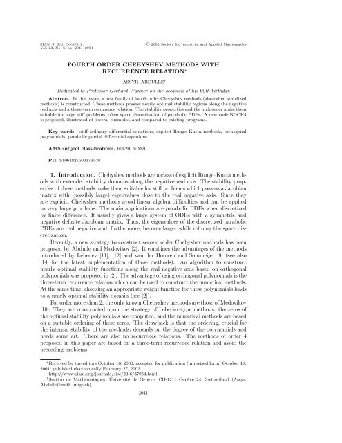
FOURTH ORDER CHEBYSHEV METHODS WITH
RECURRENCE RELATION ∗
ASSYR ABDULLE †
Dedicated to Professor Gerhard Wanner on the occasion of his 60th birthday
Abstract. In this paper, a new family of fourth order Chebyshev methods (also called stabilized
methods) is constructed. These methods possess nearly optimal stability regions along the negative
real axis and a three-term recurrence relation. The stability properties and the high order make them
suitable for large stiff problems, often space discretization of parabolic PDEs. A new code ROCK4
is proposed, illustrated at several examples, and compared to existing programs.
Key words. stiff ordinary differential equations, explicit Runge–Kutta methods, orthogonal
polynomials, parabolic partial differential equations
AMS subject classifications. 65L20, 65M20
PII. S1064827500379549
1. Introduction. Chebyshev methods are a class of explicit Runge–Kutta methods
with extended stability domains along the negative real axis. The stability properties
of these methods make them suitable for stiff problems which possess a Jacobian
matrix with (possibly large) eigenvalues close to the real negative axis. Since they
are explicit, Chebyshev methods avoid linear algebra difficulties and can be applied
to very large problems. The main applications are parabolic PDEs when discretized
by finite difference. It usually gives a large system of ODEs with a symmetric and
negative definite Jacobian matrix. Thus, the eigenvalues of the discretized parabolic
PDEs are real negative and, furthermore, become larger while refining the space discretization.
Recently, a new strategy to construct second order Chebyshev methods has been
proposed by Abdulle and Medovikov [2]. It combines the advantages of the methods
introduced by Lebedev [11], [12] and van der Houwen and Sommeijer [9] (see also
[14] for the latest implementation of these methods). An algorithm to construct
nearly optimal stability functions along the real negative axis based on orthogonal
polynomials was proposed in [2]. The advantage of using orthogonal polynomials is the
three-term recurrence relation which can be used to construct the numerical methods.
At the same time, choosing an appropriate weight function for these polynomials leads
to a nearly optimal stability domain (see [2]).
For order more than 2, the only known Chebyshev methods are those of Medovikov
[10]. They are constructed upon the strategy of Lebedev-type methods: the zeros of
the optimal stability polynomials are computed, and the numerical methods are based
on a suitable ordering of these zeros. The drawback is that the ordering, crucial for
the internal stability of the methods, depends on the degree of the polynomials and
needs some art. There are also no recurrence relations. The methods of order 4
proposed in this paper are based on a three-term recurrence relation and avoid the
preceding problems.
∗Received by the editors October 16, 2000; accepted for publication (in revised form) October 18,
2001; published electronically February 27, 2002.
http://www.siam.org/journals/sisc/23-6/37954.html
† Section de Mathématiques, Université de Genève, CH-1211 Genève 24, Switzerland (Assyr.
Abdulle@math.unige.ch).
2041

2042 ASSYR ABDULLE
The paper is organized as follows. In section 2 we explain how to compute nearly
optimal fourth order stability polynomials. Section 3 is devoted to the construction
of a family of numerical methods. These methods have been implemented in a new
code called ROCK4 which is briefly described in section 4. Finally, in section 5 we
present some numerical experiments and comparisons with other codes.
2. Fourth order stability polynomials. The aim is to construct a family of
polynomials of order 4 depending on the degree s, 1
Rs(z) =1+z + z2 z3 z4
+ +
2! 3! 4! + O(z5 (2.1)
),
which remain bounded by 1 as long as possible along the real negative axis, i.e.,
(2.2)
| Rs(z)| ≤1 for z ∈ [− ls, 0],
with ls as large as possible. It is proved in [1] that fourth order optimal stability
polynomials (which exist and are unique see [13]) possess exactly four complex zeros.
Thus, they can be written as
(2.3)
Rs(z) = w4(z) Ps−4(z),
where w4(z) =(1−/t1)(1−/¯t1)(1−/t2)(1−/¯t2), ti are complex (conjugate) numbers,
and Ps−4(z) possesses only real zeros. The idea developed in [2] for second order is
to approximate these polynomials by
(2.4)
Rs(z) =w4(z)Ps−4(z),
where w4(z) =(1− /z1)(1 − /¯z1)(1 − /z2)(1 − /¯z2) and Ps−4(z) is an orthogonal
polynomial associated with the weight function w4(z) 2 / √ 1 − z 2 . Wewanttofind
such a decomposition which satisfies (2.2) for z ∈ [−ls, 0] with ls close to ls. At the
same time, we want that the product satisfies the fourth order conditions (2.1).
The motivation for considering such polynomials can be found in [2]. Notice that
for first order optimal polynomials we have a formula similar to (2.3), with w(z) =1
and Rs(z) =Ts(1 + z
s 2 ), where Ts(z) are the Chebyshev polynomials. These optimal
polynomials are at the same time orthogonal with respect to the weight function
1/ √ 1 − z 2 . The arguments developed in [2] show that for order 2 the polynomials
(2.3) and (2.4) are very close. These arguments can be generalized for even orders
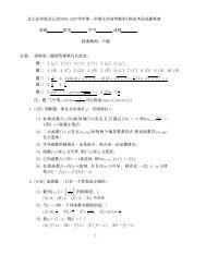
higher than 2. Figure 2.1 shows for s = 9 the difference between a fourth order
optimal stability polynomial and its approximation. We see that they can hardly be
distinguished.
For second order, the algorithm for computing the orthogonal polynomials and
the zeros of the function w(z) of (2.4) was given in [2]. We adapt here this algorithm
for order 4.
In the following we will work in the normalized interval [−1, 1] instead of [−ls, 0]
by setting x =1+ 2z
ls (ls is the length of the stability domain along R − we want to
optimize), and we take the same notation for the shifted polynomials except for the
fact that we use the variable x instead of z. Thus, we are searching for order 4 at
x = 1 (see below). If we shift the polynomials defined by (2.4) and normalize them
1 We use the notation Rs because we reserve Rs for the stability polynomials we will construct.

FOURTH ORDER CHEBYSHEV METHODS 2043
0
−20 −10 0
1
−1
Fig. 2.1. R9(x) and its stability domain, with R9(x) in the dotted line, η =0.95 (damping).
such that |w4(x)Ps−4(x)| ≤1 for x ∈ [−1, 1], then w4(1)Ps−4(1) is usually not equal
to 1. As in [2], we therefore introduce a parameter a close to 1, set
(2.5)
Rs(x) = w4(x)Ps−4(x)
w4(a)Ps−4(a) ,
and we search fourth order conditions at the point a. We denote the complex zeros
of w4(x) byx1 = α + iβ, ¯x1 = α − iβ, x2 = γ + iδ, ¯x2 = γ − iδ, and to emphasize
the dependence of Rs(x) onα, β, γ, δ we will write Rs(x, α, β, γ, δ). We have now an
optimization problem.
Problem. Find a, d, α, β, γ, δ (depending on s) such that
(2.6)
(2.7)
(2.8)
(2.9)
R ′ s(a, α, β, γ, δ) =d, R ′′
s (a, α, β, γ, δ) =d 2 ,
R ′′′
s (a, α, β, γ, δ) =d 3 , R (4)
s (a, α, β, γ, δ) =d 4 ,
|Rs(x)| ≤1 for x ∈ [−1,a]
If we then set z =(x − a)/d, we will have
(2.10)
(2.11)
with ls =(1+a)d as large as possible.
−10
Rs(0)=1, R ′ s(0)=1, R ′′
s (0)=1, R ′′′
s (0)=1, R (4)
s (0)=1,
|Rs(z)| ≤1 for z ∈ [−ls, 0].
Here again we used the same notation for the shifted polynomials. For more details
about this algorithm we refer the reader to [2].
We have computed the parameters ls,α,β,γ,δ,a (depending on s) for degree 5
up to degree more than 1000. In practice the bound in (2.8) should be replaced by
a value η

2044 ASSYR ABDULLE
Table 2.1
The stability parameters of Rs(x).
Degree Stability Value Degree Stability Value
s region ls c(s) =ls/s 2 s region ls c(s) =ls/s 2
5 5.9983 0.239931 100 3538.1276 0.353813
10 32.4470 0.324470 250 22184.4995 0.354952
20 138.3586 0.345897 500 88746.9995 0.354988
50 879.8864 0.351955 750 199684.4999 0.354995
3. Fourth order Chebyshev methods. In the preceding section we have explained
how to compute our stability polynomials. Assume now that we have such a
family of fourth order polynomials (depending on the degree s)
(3.1)
which satisfy
(3.2)
Rs(z) =w4(z)Ps−4(z),
|Rs(z)| ≤1 for z ∈ [−ls, 0],
where w4(z) =(1− /z1)(1 − /¯z1)(1 − /z2)(1 − /¯z2) and Ps−4(z) is an orthogonal
polynomial associated with the weight function
(3.3)
w4(z) 2 / 1 − z 2 ,
and normalized such that Ps−4(0) = 1. For a given degree s we will further use the
family of orthogonal polynomials (Pj) s−4
j=0 associated with the weight function (3.3),
normalized such that Pj(0) = 1. These polynomials possess a three-term recurrence
relation
Pj(z) =(µjz − νj)Pj−1(z) − κjPj−2(z).
In [2] it was explained how to compute explicitly these polynomials, given the zeros
of the function (3.3). The same procedure can be applied here, and the recurrence
coefficients can be computed simply by solving a linear system.
For second order methods, it is sufficient to construct a numerical method which
is of order 2 for linear problems, since the order conditions are the same for both linear
and nonlinear problems. This is not true for orders larger than 2, and it is therefore
not sufficient to consider only the linear case. Here we have to give a realization of our
weight function w4(z) so that the order conditions up to order 4 (8 conditions) are
satisfied. As in [10] we will use the theory of composition of methods (the “Butcher
group”) to realize fourth order Runge–Kutta–Chebyshev methods.
Suppose that we have two Runge–Kutta methods. The idea of composition of
methods is to apply one method after the other to an initial value y0 with the same
step size. The result of this process can be interpreted as a large Runge–Kutta
method: a composition of the two latter methods. For the theory of composition of
Runge–Kutta methods, we refer to [3],[6, pp. 264–273],[5].
To construct a fourth order Runge–Kutta method with the polynomials (3.1) we
proceed as follows:
• We construct a first method, denoted by P , which possesses Ps−4(z) as stability
polynomial.
• We then determine a second method, denoted by W , which possesses w4(z)
as stability polynomial, to achieve fourth order for the “composite” method
denoted by WP.

0
c2
.
a21
.
FOURTH ORDER CHEBYSHEV METHODS 2045
. ..
cs−4 as−4,1 ... as−4,s−5
b1 ... bs−5
bs−4
0
c2 a21
c3 a31 a32
c4 a41 a42 a43
Fig. 3.1. Tableau of the method P (left) and W (right).
The resulting method will be of order 4 and will possess Rs(z) =w4(z)Ps−4(z) as
stability polynomial.
Thefirst method. To construct the method P we apply a procedure similar
to that used in [2]. That is, the three-term recurrence relation of the orthogonal
is used to define the internal stages of the method as follows:
polynomials (Pj) s−4
j=1
(3.4)
g0 := y0,
g1 := y0 + hµ1f(g0),
gj := hµjf(gj−1) − νjgj−1 − κjgj−2, j =2,... ,s− 4,
y1 := gs−4.
Applied to y ′ = λy with z = hλ yields
(3.5)
gs−4 = Ps−4(z)g0.
This method is given in the left tableau of Figure 3.1. The coefficients of the method
P can be expressed recursively in term of the coefficients νj,µj,κj. Indeed, using the
notation ki = f(y0 + h i−1
j=1 aijkj) (autonomous form), we obtain for the first stage
(3.6)
g1 = y0 + hµ1f(y0) =y0 + ha21k1;
this yields a21 = µ1. For the second stage we have
(3.7)
g2 =
=
hµ2f(y0 + ha21k1) − ν2(y0 + ha21k1) − κ2y0
y0(−ν2 − κ2)+h(−ν2a21)k1 + hµ2k2;
hence a31 = −ν2a21 and a32 = µ2. (Notice that −ν2 − κ2 = 1 because of the
normalization Pj(0) = 1.) The third stage is then given by
g3 = hµ3f(y0 + h(ã31k1 +ã32k2)) − ν3(y0 + h(ã31k1 +ã32k2)) − κ3(y0 + hã21k1)
= y0(−ν3 − κ3)+h(−ν3ã31 − κ3ã21)k1 + h(−ν3ã32)k2 + hµ3k3,
and thus ã41 = −ν3ã31 − κ3ã21, ã42 = −ν3ã32 and ã43 = µ3. By induction we obtain
the following lemma.
Lemma 3.1. For the method P given by (3.4) the coefficients aij, bi, ci of the
corresponding Runge–Kutta method are given by
(3.8)
ai,j = −νi−1ai−1,j − κi−1ai−2,j, j ≤ i − 2, i ≤ s − 3(ajj := 0),
ai,i−1
bj =
=
µi−1,
as−3,j,
i ≤ s − 3,
1 ≤ j ≤ s − 4,
and the ci satisfy the usual relation ci = i−1
j=1 aij.
We emphasize that the coefficients ãij, ˜ bi will be used only to compute the method
W . For the implementation of the method, formulas (3.4) will be used.
b1
b2
b3
b4

2046 ASSYR ABDULLE
0
c2
.
a21
.
. ..
cs−4 as−4,1 ... as−4,s−5
bi b1 ... bs−3
bi + c2
b1 ... bs−3 .
bi + c4
.
b1 ... bs−3
b1 ... bs−3
bs−4
bs−4 a21
. ..
bs−4 a41 ... a43
bs−4
Fig. 3.2. Tableau of method WP.
b1 ... b3
The second and the “composite” methods. For the method W we take a
fourth stage method (right tableau of Figure 3.1) so that the composite method WP is
given by Figure 3.2. In the tableau of method WP, we will denote by ci the elements
of the first column, by aij the elements of the “triangle,” and by bi the elements of
the last row. The order conditions of the method WP are the usual ones for order 4:
(3.9)
wp( ) = bi = 1,
wp( / ) = 2 biaij = 1,
wp( \ /
) = 3 wp( /
biaijaik = 1,
\
) =
6 biaijajk = 1,
wp( \ |/
) = 4 wp( /
biaijaikail = 1,
\
\ ) = 8 wp( /
biaijajkail = 1,
\/
) = 12 wp( /
biaijajkajl = 1,
\
/
) = 24 biaijajkakl = 1.
Here we used the trees notation (connected graphs without cycles and a distinguished
vertex) for the elementary weights (wp(...)) involved in the order conditions (see [6,
pp. 145–154] or [3]).
Theorem 12.6 of [6, p. 267] can be used to express the order conditions of the
method WP in function of the two submethods, W and P . See also [5] for a new
simple proof of this latter theorem (with another normalization for the elementary
weights). We obtain
wp( ) = w( )+p( ),
wp( / ) = w( / )+2w( )p( )+p( / ),
wp( \ /
) = w( \ /
)+3w( / )p( )+3w( )p( ) 2 + p( \ /
wp( /
),
\
) =
\
w( /
)+3w( / )p( )+3w( )p( / )+p( / \
),
wp( \ |/
) = w( \ |/
)+4w( \ /
)p( )+6w( / )p( ) 2 +4w( )p( ) 3 + p( \ |/
),
b4

FOURTH ORDER CHEBYSHEV METHODS 2047
w( /\
2 )p( )+
\ )p( ))+6( 1
3w( / )p( / )+ 2
3w( / )p( ) 2 )
wp( / \
\ ) = w( / \
\ )+4( 1
3 3w( /
+4w( )p( )p( / )+p( / \
\ ),
wp( / \/
) = w( / \/
)+4w( / \
)p( )+6w( / )p( ) 2 +4w( )p( \ /
)+p( / \/
wp( / \
/
) = w( / \
/
)+4w( / \
)p( )+6w( / )p( / )+4w( )p( / \
\
)+p( /
/
where w(...) and p(...) are the expressions (3.9) for the methods W and P , respectively.
These formulas allow us to compute recursively the expressions w( ),w(/ ),...
for the method W , since the expressions p( ),p(/ ),... can be computed with the coefficients
of the method P given by (3.8). This leads to the following equations for
the method W :
(3.10)
b1 + b2 + b3 + b4 = w( ),
b2c2 + b3c3 + b4c4 = w(/ )
2 ,
b2c 2 2 + b3c 2 3 + b4c 2
w( /
4 =
\ )
3 ,
b3a32c2 + w( /\
b4(a42c2 + a43c3) =
)
6 ,
b2c 3 2 + b3c 3 3 + b4c 3 4 = w( \ |/
)
4 ,
b3c3a32c2 + b4c4(a42c2 + a43c3) =
b3a32c 2 2 + b4(a42c 2 2 + a43c 2 3) =
b4a43a32c2 =
w( \ /\ )
8 ,
w( /\/
)
12 ,
/
w( /\ )
24 .
This is a system of 8 equations for 10 unknowns bi, aij (ci are determined by ci =
i−1
j=1 aij.) These equations are similar to the equations of usual fourth order methods
(i.e., when w( ) =1,w(/ )=1, ...; see [6, pp. 135–136]). We have two degrees of
freedom, and we choose c3 =
w( )
3
and c4 =
2w( )
3
),
after some experimentation. This
choice keeps the absolute value of the coefficients bi, aij less than 1, which is suitable
for a numerical method.
The solution of equations (3.10) gives us the coefficients of the method W . Thus,
we have obtained a family of methods (depending on the degree of the stability polynomial)
of order 4 with recurrence formulas and with the polynomial (3.1) as a stability
function.
The embedded method. For the estimation of the local error of the constructed
numerical method
⎛
⎞
(3.11)
s
i−1
y1 = y0 + h bif ⎝y0 + h
s
⎠ = y0 + h biki,
i=1
j=1
aijkj
we use an embedded method of order 3.
Since for fourth order methods there is no embedded method of order 3 using the
same function values ki = f(y0 + h aijkj) (see [6, p. 167]), we search for a lower
i=1
),

2048 ASSYR ABDULLE
0
c2 a21
c3 a31 a32
c4 a41 a42 a43
c5
order method of the form
(3.12) ⎛ ⎛
s
i−1
y1 = y0 + h ⎝ βif ⎝y0 + h
i=1
b1
¯ b1
b2
¯ b2
b3
¯ b3
b4
¯ b4
¯ b5
Fig. 3.3. Tableau of the method W .
j=1
aijkj
⎞
⎞
s
⎠ + βs+1f(y1) ⎠ = y0 + h
i=1
βiki + βs+1ks+1
This is no extra work (if the step is accepted) because f(y1) has to be computed
anyway for the next stage. As a measure of the error after one step we will take
(3.13)
err = y1 − y 1.
We want to keep the recurrence formulas for the embedded method. Therefore,
the embedded method will be a composition of the method P , defined in (3.4), with
a new method W denoted by W . For that, we add a fifth stage to the method W
as shown in Figure 3.3. Similarly to (3.10) we derive third order conditions for the
method W :
(3.14)
¯ b1 + ¯ b2 + ¯ b3 + ¯ b4 + ¯ b5 = w( ),
¯b2c2 + ¯b3c3 + ¯b4c4 + ¯b4c5 = w(/ )
2 ,
¯b2c 2 2 + ¯b3c 2 3 + ¯b4c 2 4 + ¯b5c 2
w( /
5 =
\ )
3 ,
¯b3a32c2 + ¯b4(a42c2 + a43c3)+ ¯b5( b2c2 + b3c3 + w( /\
b4c4) =
)
6 .
Notice that c5 = bi = w( ). The last equation of (3.14) can be simplified since
b2c2 + b3c3 + b4c4 = w(/ )
2 (see (3.10)). We obtain a system of 4 equations for 5
unknowns ¯ bi. We require the following additional condition:
(3.15)
¯w5(−ls) =0,
where ¯w5(z) is the stability polynomial of the method W and ls the length of the
stability domain along the negative real axis (see (3.2)).
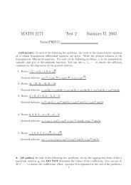
Solving (3.14) and (3.15), numerical computations show that the stability polynomials
of the embedded methods are bounded (by η =0.95) on the same interval as
the stability polynomials of the numerical methods (see Figure 3.4). There is a simple
criterion to check if ¯ Rs+1(z), the stability polynomials of the embedded method,
is bounded by η on the same interval as Rs(z). Recall that Rs(z) =w4(z)Ps−4(z)
.

0
−40 −30 −20 −10 0
FOURTH ORDER CHEBYSHEV METHODS 2049
1
−1
0
−60 −50 −40 −30 −20 −10 0
Fig. 3.4. Stability polynomials of the method WP and the embedded method WP (dotted line)
for s =9(left) and s =13(right).
and ¯ Rs+1(z) = ¯w5(z)Ps−4(z). Denote by zi the zeros of Ps−4(z). Because Ps−4(z)
is an orthogonal polynomial its zeros are simple and all in the stability interval, say
−ls 0 such that | ¯ Rs+1(z)| > |Rs(z)|
for z ∈ (z1,z1 + ɛ). Since ¯ Rs+1(−ls) =0,d(z) must have a double zero at z1 or vanish
at least once in (−ls,z1). In both cases, counting the zeros of d(z) outside of the
origin leads to a contradiction.
4. Description of ROCK4. We implemented the numerical method described
in section 3 in a code called ROCK4 for Orthogonal-Runge–Kutta–Chebyshev (appropriately
permuted). This is the fourth order version of the code ROCK2 introduced
in [2]. In this section we briefly describe the code.
Step size estimation. As in ROCK2, we implemented the “step size strategy with
memory” of Watts [16] and Gustafsson [4],
(4.1)
hnew = fac · hn
1
errn+1
1
4 hn
hn−1
errn
errn+1
1
4
,
in order to allow the step size to decrease reasonably without rejection (see also [7,
p. 124]).
Stage number selection. While most stiff codes have a fixed number of stages, we
used, as usual in Chebyshev codes, a family of fourth order methods. At each step we
first select a step size in order to control the local error; then we select a stage order
so that the stability property (see section 2 and Table 2.1)
∂f
hρ
∂y (y)
≤ 0.35s 2
(4.2)
1
−1

2050 ASSYR ABDULLE
is satisfied, where ρ(...) denotes the spectral radius of the Jacobian matrix of the
ODEs. This is possible because for practical purposes, the error constants of the
family of fourth order methods are found to be almost the same. They are close to
the error constants of optimal stability polynomials which have been described in [1].
Spectral radius estimate. The user can supply a function which estimates a bound
for the spectral radius (for example, by using Gershgorin theorem; see [6, p. 89]). By
specifying that the Jacobian is constant, this function will be called only once. If it
is not possible to get an estimate of the spectral radius easily, the code ROCK4 can
also compute it internally. For that, we have implemented with a slight modification
a nonlinear power method proposed by Sommeijer, Shampine, and Verwer (see [14]).
Storage. Due to the three-term recurrence formula, the method requires only a
few storage vectors. The number of storage vectors does not depend on the number
of stages used. For the computation of an integration step and the error estimation,
ROCK4 uses three vectors for the recurrence formula and five additional vectors for
the finishing four-stage method and the embedded method. Notice that the low
memory demand of these methods is suitable since we want to apply them to large
problems.
5. Numerical experiments. We conclude this paper with several stiff problems
taken from the test set of stiff problems proposed in [7] (first and second editions). All
the parameters chosen for the examples are taken from [7]. We compare the following
codes:
ROCK4: the fourth order code described in this paper.
ROCK2: the second order code based on orthogonal polynomials and described
in [2].
RKC: the second order Chebyshev code of Sommeijer, Shampine, and Verwer (see
[14]).
RADAU5: the well-known implicit code by Hairer and Wanner of order 5 based
on a Radau IIA collocation method (see [7]).
For all examples which follow, we compared the obtained numerical results for
the different codes with a reference solution for the given ODEs. The computing time
is then displayed as a function of the error (in an Euclidian norm). For each problem
the codes have been applied with different tolerances, say
(5.1)
tol =10 −2 1
1
−2−
, 10 4 −2−
, 10 2 ,... .
The integer-exponent tolerances are displayed as enlarged symbols. The results were
computed with scalar tolerances atol = rtol = tol for all problems. The symbol for
tol =10 −5 is distinguished by its gray color.
The following examples are parabolic PDEs, discretized by the method of line
into a system of ODEs. We replace the second order spatial derivatives by the finite
difference scheme
∂ 2 u(xi,yj,t)
∂x 2
= ui+1,j − 2ui,j + ui−1,j
(∆x) 2
where uij are functions depending on time.
Example 1. The first example is the Burgers’ equation
2 u
(5.2)
ut + = µuxx,
2
x
+ O (∆x) 2 ,

with initial condition
(5.3)
and boundary conditions
(5.4)
FOURTH ORDER CHEBYSHEV METHODS 2051
u(x, 0)=1.5x(1 − x) 2 ,
u(0,t)=u(1,t)=0
for 0 ≤ x ≤ 1 and 0 ≤ t ≤ 2.5. We discretize the space variable of (5.2) by the method
of lines with ∆x = 1
501 , and we choose µ =0.0003.
10 1
10 0
10 −1
sec
BURGERS SMOOTH
RADAU5
RKC
ROCK2
ROCK4
10 0 10 −3 10 −6 10 −9
error
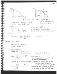
Fig. 5.1. Work-precision diagram for Burgers’ equations.
Thus, we obtain an ODE (in time) of dimension 500. It is then solved by the
different codes for 0 ≤ t ≤ 2.5. For RADAU5 we used the banded algebra option, and
for the Chebyshev codes we provide an estimation of the spectral radius by applying
the Gershgorin theorem.
We see in Figure 5.1 that the two lower order methods, RKC and ROCK2, are
better for lower tolerances. ROCK2 is slightly more efficient and better at delivering
an accuracy close to the tolerance. For higher tolerances the high order codes
RADAU5 and ROCK4 are better, with an advantage for ROCK4. This latter code
also nicely preserves the tolerance proportionality.
Example 2. The second example is the two-dimensional Brusselator reactiondiffusion
problem
∂u
∂t = 1+u2 2 ∂ u
v − 4.4u + α
∂x2 + ∂2u ∂y2
+ f(x, y, t),
∂v
∂t = 3.4u − u2 2 ∂ v
v + α
∂x2 + ∂2v ∂y2 (5.5)
,

2052 ASSYR ABDULLE
10 4
10 3
sec
BRUSS-2D
ROCK2
RKC
RADAU5
ROCK4
error
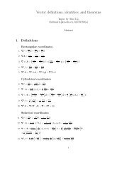
100 10−3 10−6 10−9 10−12 102 Fig. 5.2. Work-precision diagram for the two-dimensional Brusselator problem.
with initial conditions
u(x, y, 0)=22· y(1 − y) 3/2 , v(x, y, 0)=27· x(1 − x) 3/2 ,
and periodic boundary conditions
u(x +1,y,t)=u(x, y, t), u(x, y +1,t)=u(x, y, t)
for 0 ≤ x ≤ 1, 0 ≤ y ≤ 1, t≥ 0. The function f is defined by
2 2 2 5 if (x−0.3) +(y − 0.6) ≤ 0.1 and t ≥ 1.1,
f(x, y, t) =
0 else.
We discretize the space variables of equations (5.5) with xi = i
N+1 ,yi = i
N+1 ,i=
1, 2,... ,N and choose N = 128 and α =0.1. Thus, we obtain a system of 2N 2 =
32768 equations. We chose the output points t out =1.5 and 11.5. The spectral radius
of the Jacobian ρ 13200 can be estimated with the Gershgorin theorem; thus as in
the previous example, we provide a bound for it when using Chebyshev methods. As
advised in [7, p. 157] the linear equations in the code RADAU5 are solved by FFT
methods so that the code is optimized for this problem. (Otherwise it will certainly
not be competitive with Chebyshev methods.)
We see in Figure 5.2 that ROCK2 and RKC behaves similarly. For higher order
methods, RADAU5 behaves better for low tolerances, while ROCK4 is better for
higher tolerances. Between Chebyshev codes, except for very low tolerances ROCK4
gives the best results and nicely preserves the tolerance proportionality (as do ROCK2
and RADAU5).
Example 3. The third example is the FitzHugh and Nagumo model for explaining

10 1
10 0
FOURTH ORDER CHEBYSHEV METHODS 2053
sec
RKC
FINAG
ROCK2
RADAU5
ROCK4
error
10 0 10 −3 10 −6 10 −9
Fig. 5.3. Work-precision diagram for FitzHugh and Nagumo equations.
the nerve conduction as a traveling wave:
(5.6)
where
with initial conditions
and boundary conditions
∂u
∂x (0,t)=−0.3,
for 0 ≤ x ≤ 100 and 0 ≤ t ≤ 400.
∂u
∂t = ∂2u − f(u) − v,
∂x2 ∂v
∂t
= η(u − βv),
f(u) =u(u − α)(u − 1),
u(x, 0) = v(x, 0)=0,
∂u
∂x (100,t)=0
We chose α =0.139, η =0.008, and β =2.54 and discretize the space variable in
200 equidistant steps xi = 2i+1
4 ,i=0,...,199. We compute numerically a bound for
the spectral radius of the Jacobian which was used for the Chebyshev methods. This
is a mildly stiff problem, and we see in Figure 5.3 the advantage of the Chebyshev
methods compared to an implicit one. Again, ROCK2 works slightly better than
RKC. ROCK4 behaves well and is better compared to other Chebyshev methods
even for low tolerances.

2054 ASSYR ABDULLE
Conclusion. We have presented a new fourth order Chebyshev method and implemented
it in a code called ROCK4. The numerical examples show a good behavior
of this code for problems it is intended for. We emphasize that this code, as does other
Chebyshev codes, is very simple to use. In fact, it is as simple to use as the forward
Euler method. The first version of this code (as well as ROCK2) and some examples
are available on the Internet at the address http://www.unige.ch/math/folks/hairer/
software.html. Experiences with this code are welcome.
Acknowledgments. The author is grateful to Ernst Hairer and Gerhard Wanner
for helpful discussions. He also thanks Alexei Medovikov for his constant interest in
this subject.
REFERENCES
[1] A. Abdulle, On roots and error constant of optimal stability polynomials, BIT, 40 (2000),
pp. 177–182.
[2] A. Abdulle and A.A. Medovikov, Second order Chebyshev methods based on orthogonal
polynomials, Numer. Math., 90 (2001), pp. 1–18.
[3] J.C. Butcher, The Numerial Analysis of Ordinary Differential Equations. Runge-Kutta and
General Linear Methods, John Wiley and Sons, Chichester, UK, 1987.
[4] K. Gustafsson, Control-theoretic techniques for stepsize selection in implicit Runge-Kutta
methods, ACM Trans. Math. Software, 20 (1994), pp. 496–517.
[5] E. Hairer, C. Lubich, and G. Wanner, Geometric Numerical Integration, Springer-Verlag,
Berlin, Heidelberg, New York, 2002.
[6] E. Hairer, S.P. Nørsett, and G. Wanner, Solving Ordinary Differential Equations I. Nonstiff
Problems, 2nd ed., Springer Ser. Comput. Math. 8, Springer-Verlag, Berlin, 1993.
[7] E. Hairer and G. Wanner, Solving Ordinary Differential Equations II. Stiff and Differential-
Algebraic Problems, 2nd ed., Springer Ser. Comput. Math. 14, Springer-Verlag, Berlin,
1996.
[8] P.J. van der Houwen, Construction of Integration Formulas for Initial Value Problems,
North-Holland, Amsterdam, 1977.
[9] P.J van der Houwen and B.P. Sommeijer, On the internal stability of explicit m-stage
Runge-Kutta methods for large m-values, Z. Angew. Math. Mech., 60 (1980), pp. 479–485.
[10] A.A. Medovikov, High order explicit methods for parabolic equations, BIT, 38 (1998), pp. 372–
390.
[11] V.I. Lebedev, A new method for determining the zeros of polynomials of least deviation on a
segment with weight and subject to additional conditions. Part I, Russian J. Numer. Anal.
Math. Modelling., 8 (1993), pp. 195–222.
[12] V.I. Lebedev, A new method for determining the zeros of polynomials of least deviation on a
segment with weight and subject to additional conditions. Part II, Russian J. Numer. Anal.
Math. Modelling., 8 (1993), pp.397–426.
[13] W. Riha, Optimal stability polynomials, Computing, 9 (1972), pp. 37–43.
[14] B.P. Sommeijer, L.F. Shampine, and J.G. Verwer, RKC: An explicit solver for parabolic
PDEs, J. Comput. Appl. Math., 88 (1998) pp. 316–326.
[15] J.W. Verwer, Explicit Runge-Kutta methods for parabolic partial differential equations, Appl.
Numer. Math., 22 (1996), pp. 359–379.
[16] H.A. Watts, Step size control in ordinary differential equation solvers, Trans. Soc. Computer
Simulation, 1 (1984) pp. 15–25.