fourth order chebyshev methods with recurrence relation

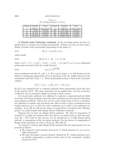
2044 ASSYR ABDULLE
Table 2.1
The stability parameters of Rs(x).
Degree Stability Value Degree Stability Value
s region ls c(s) =ls/s 2 s region ls c(s) =ls/s 2
5 5.9983 0.239931 100 3538.1276 0.353813
10 32.4470 0.324470 250 22184.4995 0.354952
20 138.3586 0.345897 500 88746.9995 0.354988
50 879.8864 0.351955 750 199684.4999 0.354995
3. Fourth order Chebyshev methods. In the preceding section we have explained
how to compute our stability polynomials. Assume now that we have such a
family of fourth order polynomials (depending on the degree s)
(3.1)
which satisfy
(3.2)
Rs(z) =w4(z)Ps−4(z),
|Rs(z)| ≤1 for z ∈ [−ls, 0],
where w4(z) =(1− /z1)(1 − /¯z1)(1 − /z2)(1 − /¯z2) and Ps−4(z) is an orthogonal
polynomial associated with the weight function
(3.3)
w4(z) 2 / 1 − z 2 ,
and normalized such that Ps−4(0) = 1. For a given degree s we will further use the
family of orthogonal polynomials (Pj) s−4
j=0 associated with the weight function (3.3),
normalized such that Pj(0) = 1. These polynomials possess a three-term recurrence
relation
Pj(z) =(µjz − νj)Pj−1(z) − κjPj−2(z).
In [2] it was explained how to compute explicitly these polynomials, given the zeros
of the function (3.3). The same procedure can be applied here, and the recurrence
coefficients can be computed simply by solving a linear system.
For second order methods, it is sufficient to construct a numerical method which
is of order 2 for linear problems, since the order conditions are the same for both linear
and nonlinear problems. This is not true for orders larger than 2, and it is therefore
not sufficient to consider only the linear case. Here we have to give a realization of our
weight function w4(z) so that the order conditions up to order 4 (8 conditions) are
satisfied. As in [10] we will use the theory of composition of methods (the “Butcher
group”) to realize fourth order Runge–Kutta–Chebyshev methods.
Suppose that we have two Runge–Kutta methods. The idea of composition of
methods is to apply one method after the other to an initial value y0 with the same
step size. The result of this process can be interpreted as a large Runge–Kutta
method: a composition of the two latter methods. For the theory of composition of
Runge–Kutta methods, we refer to [3],[6, pp. 264–273],[5].
To construct a fourth order Runge–Kutta method with the polynomials (3.1) we
proceed as follows:
• We construct a first method, denoted by P , which possesses Ps−4(z) as stability
polynomial.
• We then determine a second method, denoted by W , which possesses w4(z)
as stability polynomial, to achieve fourth order for the “composite” method
denoted by WP.