fourth order chebyshev methods with recurrence relation
fourth order chebyshev methods with recurrence relation
fourth order chebyshev methods with recurrence relation

You also want an ePaper? Increase the reach of your titles
YUMPU automatically turns print PDFs into web optimized ePapers that Google loves.
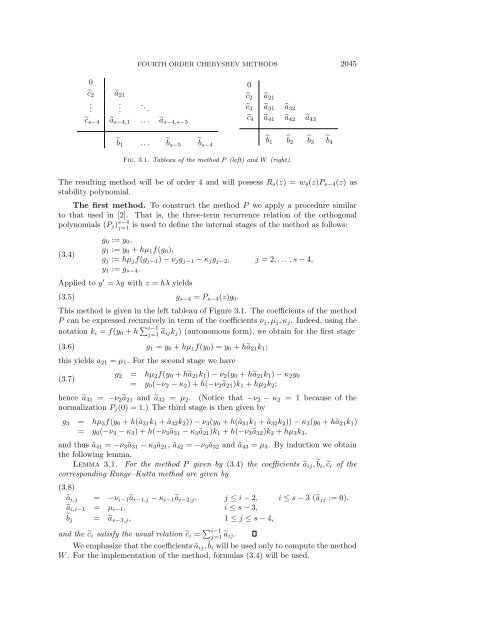
0<br />
c2<br />
.<br />
a21<br />
.<br />
FOURTH ORDER CHEBYSHEV METHODS 2045<br />
. ..<br />
cs−4 as−4,1 ... as−4,s−5<br />
b1 ... bs−5<br />
bs−4<br />
0<br />
c2 a21<br />
c3 a31 a32<br />
c4 a41 a42 a43<br />
Fig. 3.1. Tableau of the method P (left) and W (right).<br />
The resulting method will be of <strong>order</strong> 4 and will possess Rs(z) =w4(z)Ps−4(z) as<br />
stability polynomial.<br />
Thefirst method. To construct the method P we apply a procedure similar<br />
to that used in [2]. That is, the three-term <strong>recurrence</strong> <strong>relation</strong> of the orthogonal<br />
is used to define the internal stages of the method as follows:<br />
polynomials (Pj) s−4<br />
j=1<br />
(3.4)<br />
g0 := y0,<br />
g1 := y0 + hµ1f(g0),<br />
gj := hµjf(gj−1) − νjgj−1 − κjgj−2, j =2,... ,s− 4,<br />
y1 := gs−4.<br />
Applied to y ′ = λy <strong>with</strong> z = hλ yields<br />
(3.5)<br />
gs−4 = Ps−4(z)g0.<br />
This method is given in the left tableau of Figure 3.1. The coefficients of the method<br />
P can be expressed recursively in term of the coefficients νj,µj,κj. Indeed, using the<br />
notation ki = f(y0 + h i−1<br />
j=1 aijkj) (autonomous form), we obtain for the first stage<br />
(3.6)<br />
g1 = y0 + hµ1f(y0) =y0 + ha21k1;<br />
this yields a21 = µ1. For the second stage we have<br />
(3.7)<br />
g2 =<br />
=<br />
hµ2f(y0 + ha21k1) − ν2(y0 + ha21k1) − κ2y0<br />
y0(−ν2 − κ2)+h(−ν2a21)k1 + hµ2k2;<br />
hence a31 = −ν2a21 and a32 = µ2. (Notice that −ν2 − κ2 = 1 because of the<br />
normalization Pj(0) = 1.) The third stage is then given by<br />
g3 = hµ3f(y0 + h(ã31k1 +ã32k2)) − ν3(y0 + h(ã31k1 +ã32k2)) − κ3(y0 + hã21k1)<br />
= y0(−ν3 − κ3)+h(−ν3ã31 − κ3ã21)k1 + h(−ν3ã32)k2 + hµ3k3,<br />
and thus ã41 = −ν3ã31 − κ3ã21, ã42 = −ν3ã32 and ã43 = µ3. By induction we obtain<br />
the following lemma.<br />
Lemma 3.1. For the method P given by (3.4) the coefficients aij, bi, ci of the<br />
corresponding Runge–Kutta method are given by<br />
(3.8)<br />
ai,j = −νi−1ai−1,j − κi−1ai−2,j, j ≤ i − 2, i ≤ s − 3(ajj := 0),<br />
ai,i−1<br />
bj =<br />
=<br />
µi−1,<br />
as−3,j,<br />
i ≤ s − 3,<br />
1 ≤ j ≤ s − 4,<br />
and the ci satisfy the usual <strong>relation</strong> ci = i−1<br />
j=1 aij.<br />
We emphasize that the coefficients ãij, ˜ bi will be used only to compute the method<br />
W . For the implementation of the method, formulas (3.4) will be used.<br />
b1<br />
b2<br />
b3<br />
b4