Inverse Reinforcement Learning with PI
Inverse Reinforcement Learning with PI
Inverse Reinforcement Learning with PI

You also want an ePaper? Increase the reach of your titles
YUMPU automatically turns print PDFs into web optimized ePapers that Google loves.
<strong>Inverse</strong> <strong>Reinforcement</strong> <strong>Learning</strong> <strong>with</strong> <strong>PI</strong> 2<br />
Mrinal Kalakrishnan, Evangelos Theodorou, and Stefan Schaal<br />
Department of Computer Science, University of Southern California<br />
INTRODUCTION<br />
We present an algorithm that recovers an unknown cost<br />
function from expert-demonstrated trajectories in continuous<br />
space. We assume that the cost function is a weighted linear<br />
combination of features, and we are able to learn weights that<br />
result in a cost function under which the expert demonstrated<br />
trajectories are optimal. Unlike previous approaches [1],<br />
[2], our algorithm does not require repeated solving of the<br />
forward problem (i.e., finding optimal trajectories under a<br />
candidate cost function). At the core of our approach is the<br />
<strong>PI</strong> 2 (Policy Improvement <strong>with</strong> Path Integrals) reinforcement<br />
learning algorithm [3], which optimizes a parameterized<br />
policy in continuous space and high dimensions. <strong>PI</strong> 2 boasts<br />
convergence that is an order of magnitude faster than previous<br />
trajectory-based reinforcement learning algorithms on<br />
typical problems. We solve for the unknown cost function<br />
by enforcing the constraint that the expert-demonstrated<br />
trajectory does not change under the <strong>PI</strong> 2 update rule, and<br />
hence is locally optimal.<br />
<strong>PI</strong> 2 : POLICY IMPROVEMENT WITH PATH INTEGRALS<br />
We represent all trajectories as Dynamic Movement Primitives<br />
(DMPs) [4], which are parameterized policies expressed<br />
by a set of differential equations. The DMP representation<br />
is advantageous as it guarantees attractor properties towards<br />
the goal while remaining linear in its parameters θ, thus<br />
facilitating learning [5].<br />
The <strong>PI</strong> 2 algorithm arises from a solution of the stochastic<br />
Hamilton-Jacobi-Bellman (HJB) equation using the<br />
Feynman-Kac theorem, which transforms the stochastic optimal<br />
control problem into the approximation problem of a<br />
path integral. Detailed derivations are omitted due to lack of<br />
space; we refer the reader to a previous publication [3]. We<br />
consider cost functions of the following form:<br />
Email: {kalakris, etheodor, sschaal}@usc.edu<br />
Q(τ ) = φtN +<br />
N−1 <br />
(qt + u T<br />
tRut)dt (1)<br />
i=0<br />
where Q(τ ) is the cost of a trajectory τ , φtN is the terminal<br />
cost, N is the number of time steps, qt is an arbitrary statedependent<br />
cost function, ut are the control commands at<br />
time t, and R is the positive definite weight matrix of the<br />
quadratic control cost. <strong>PI</strong>2 updates the parameters of a DMP<br />
<strong>with</strong> parameters θ, using K trajectories sampled from the<br />
same start state, <strong>with</strong> stochastic parameters θ + ɛt at every<br />
time step. The update equations are as follows:<br />
P (τ i,k) =<br />
δθti =<br />
K m=1<br />
1 − e λ S(τ i,k)<br />
1<br />
e− λ S(τ i,m)<br />
K<br />
P (τ i,k)Mti,kɛti,k<br />
k=1<br />
S(τ i,k) = φtN ,k +<br />
1<br />
2<br />
N−1 <br />
j=i+1<br />
N−1 <br />
j=i<br />
Mtj,k = R−1 gtj,kg T<br />
tj,k<br />
g T<br />
tj,k R−1 gtj,k<br />
(2)<br />
(3)<br />
qtj,kdt+ (4)<br />
(θ + Mtj,kɛtj,k) T R(θ + Mtj,kɛtj,k)dt<br />
where k indexes over the K sampled trajectories used for<br />
the update, i indexes over all time-steps, P (τ i,k) is the<br />
discrete probability of trajectory τ k at time ti, S(τ i,k) is the<br />
cumulative cost of trajectory τ k starting from time ti, δθti is<br />
the update to the DMP parameter vector at time ti, φtN ,k is<br />
the terminal cost incurred by trajectory τ k, qtj,k is the cost<br />
incurred by trajectory τ k at time tj, ɛtj,k is the noise applied<br />
to the parameters of trajectory τ k at time tj, and gtj,k are<br />
the basis functions of the DMP function approximator for<br />
trajectory τ k at time tj.<br />
INVERSE REINFORCEMENT LEARNING WITH <strong>PI</strong> 2<br />
We assume that the arbitrary state-dependent cost function<br />
qt is linearly parameterized as:<br />
qt = β T<br />
qψ t<br />
where ψ t are the feature values at time t, and β q are the<br />
weights associated <strong>with</strong> the features, which we are trying to<br />
learn. Due to the coupling of exploration noise and command<br />
cost in the path integral formalism, we assume that the the<br />
shape of the quadratic control cost matrix R is given, and<br />
we can only learn its scaling factor. We also need to learn<br />
the scaling factor on the terminal cost:<br />
(5)<br />
(6)<br />
R = βR ˆ R; φtN = βφt N ψtN (7)<br />
where βR is the control cost scaling factor that needs to be<br />
learned, ˆ R is the shape of the control cost, βφt is the scaling<br />
N<br />
of the terminal cost, and ψtN is a binary feature which is 1<br />
when the terminal state is reached, and 0 otherwise.
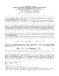
(a) (b)<br />
Fig. 1. (a) A cost function in a 2-D state space, along <strong>with</strong> a demonstrated low-cost trajectory between two points. The cost function is generated as a<br />
randomly weighted combination of some underlying features. (b) The cost function learnt from the single demonstrated trajectory.<br />
We can rewrite Eqn. 4, the cumulative cost, as follows:<br />
⎡<br />
S(τ i,k) = β T ⎣<br />
1<br />
2<br />
P N−1<br />
N−1<br />
j=i ψtj,k<br />
j=i+1 (θ + Mt j ,kɛt j ,k) T ˆ R(θ + Mt j ,kɛt j ,k)<br />
ψtN ,k<br />
= β T Φ (8)<br />
where β = [β q βR βφt N ] T is the weight vector to be<br />
learned, and Φ are sufficient statistics that can be computed<br />
for every time-step for each sample trajectory.<br />
The expert-demonstrated trajectory can be considered locally<br />
optimal under a particular cost function if the updates<br />
to its parameters using the <strong>PI</strong> 2 update rule are 0. In order<br />
to achieve the inverse, i.e., solve for the cost function under<br />
which the expert-demonstrated trajectory is locally optimum,<br />
we minimize the squared magnitude of trajectory updates,<br />
<strong>with</strong> an additional regularization term on the weight vector:<br />
minβ<br />
N−1 <br />
i=0<br />
w 2 i (δθti) T (δθti) + γβ T β (9)<br />
N − i<br />
wi = (10)<br />
N−1<br />
i=0 (N − i)<br />
where γ is a scalar regularization factor. The weights wi<br />
assign a weight to the update for each time step, equal to the<br />
number of time steps left in the trajectory. This gives early<br />
points in the trajectory a higher weight, which is useful since<br />
their parameters affect a larger time horizon. Other weighting<br />
schemes could be used, but this one was experimentally<br />
found to give good learning results [3].<br />
The solution of this optimization problem yields a weight<br />
vector β, which produces the cost function we seek. We<br />
optimize this objective function using the Matlab non-linear<br />
least squares solver, and are currently investigating alternate,<br />
more efficient ways of performing this optimization.<br />
⎤<br />
⎦<br />
EVALUATION<br />
We generated 5 random features in a 2-D state space, each<br />
feature being a sum of many Gaussians <strong>with</strong> random centers<br />
and variances. A random weighting of these features results<br />
in a cost function, shown in Fig. 1(a). A low-cost trajectory<br />
between two points is then demonstrated in this state space,<br />
also seen in Fig. 1(a). We then sampled 50 trajectories<br />
around this expert-demonstrated trajectory, and solved the<br />
optimization problem in Eqn. 9 to obtain the weights β,<br />
and the resulting cost function as seen in Fig. 1(b). There<br />
is an excellent match between the true cost function and the<br />
learned one, demonstrating the effectiveness of our approach.<br />
These results are to be considered preliminary. Efficient<br />
algorithms for optimizing Eqn. 9, systematic evaluations<br />
of learning performance, comparisons <strong>with</strong> other inverse<br />
reinforcement learning algorithms, and applications to realworld<br />
problems are left for future work.<br />
REFERENCES<br />
[1] P. Abbeel and A. Y. Ng, “Apprenticeship learning via inverse reinforcement<br />
learning,” in Proceedings of the twenty-first international<br />
conference on Machine learning, 2004.<br />
[2] N. Ratliff, D. Silver, and J. Bagnell, “<strong>Learning</strong> to search: Functional<br />
gradient techniques for imitation learning,” Autonomous Robots, vol. 27,<br />
pp. 25–53, July 2009.<br />
[3] E. A. Theodorou, J. Buchli, and S. Schaal, “<strong>Reinforcement</strong> learning<br />
of motor skills in high dimensions: A path integral approach,” in<br />
International Conference of Robotics and Automation (accepted), 2010.<br />
Available at http://www-clmc.usc.edu/publications/E/<br />
<strong>PI</strong>2.pdf.<br />
[4] A. J. Ijspeert, J. Nakanishi, and S. Schaal, “<strong>Learning</strong> attractor landscapes<br />
for learning motor primitives,” Advances in neural information<br />
processing systems, pp. 1547–1554, 2003.<br />
[5] J. Peters and S. Schaal, “<strong>Reinforcement</strong> learning of motor skills <strong>with</strong><br />
policy gradients,” Neural Networks, vol. 21, no. 4, pp. 682–697, 2008.<br />
Topic: learning algorithms; Preference: oral/poster