Riemannian Metric estimation and the problem of geometric recovery
Riemannian Metric estimation and the problem of geometric recovery
Riemannian Metric estimation and the problem of geometric recovery

You also want an ePaper? Increase the reach of your titles
YUMPU automatically turns print PDFs into web optimized ePapers that Google loves.
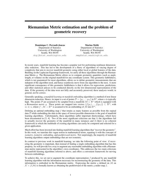
<strong>Riemannian</strong> <strong>Metric</strong> <strong>estimation</strong> <strong>and</strong> <strong>the</strong> <strong>problem</strong> <strong>of</strong><br />
<strong>geometric</strong> <strong>recovery</strong><br />
Dominique C. Perrault-Joncas<br />
Department <strong>of</strong> Statistics<br />
University <strong>of</strong> Washington<br />
Seattle, WA 98195<br />
dcpj@stat.washington.edu<br />
Marina Meilă<br />
Department <strong>of</strong> Statistics<br />
University <strong>of</strong> Washington<br />
Seattle, WA 98195<br />
mmp@stat.washington.edu<br />
In recent years, manifold learning has become a popular tool for performing nonlinear dimensionality<br />
reduction. This has led to <strong>the</strong> development <strong>of</strong> a flurry <strong>of</strong> algorithms <strong>of</strong> varying degree <strong>of</strong><br />
complexity that aim to recover manifold geometry using ei<strong>the</strong>r local or global features <strong>of</strong> <strong>the</strong> data.<br />
Building on <strong>the</strong> Laplacian Eigenmap framework, we unify all <strong>the</strong>se algorithms through <strong>the</strong> <strong>Riemannian</strong><br />
<strong>Metric</strong> g. The <strong>Riemannian</strong> <strong>Metric</strong> allows us to compute <strong>geometric</strong> quantities (such as angle,<br />
length, or volume) on <strong>the</strong> original manifold for any coordinate system. This <strong>geometric</strong> faithfulness,<br />
which is not guaranteed for most algorithms, allows us to define <strong>geometric</strong> measurements that are<br />
indepent <strong>of</strong> <strong>the</strong> algorithm used, <strong>and</strong> hence seamlessly move from one algorithm to <strong>the</strong> next. A more<br />
significant consequence <strong>of</strong> this <strong>geometric</strong> faithfulness is that it allows for regressions, predictions,<br />
<strong>and</strong> o<strong>the</strong>r statistical anlyses to be conducted directly on <strong>the</strong> low-dimensional representation <strong>of</strong> <strong>the</strong><br />
data. If <strong>the</strong> geometry <strong>of</strong> <strong>the</strong> data were not fully <strong>and</strong> accurately preserved, <strong>the</strong>se analyses would, in<br />
general, not be correct.<br />
Generally speaking, a manifold learning or manifold embedding algorithm is a method <strong>of</strong> non-linear<br />
dimension reduction. Hence, its input is a set <strong>of</strong> points D = {p1, . . . pN } in R n , where n is typically<br />
high. The points D are assumed to be sampled from a manifold M ⊂ R n which is equipped with<br />
a <strong>Riemannian</strong> metric g. These points are mapped into vectors {f(p1), . . . f(pN )} ⊂ R m , with<br />
m ≪ n, where f : M → R m is assumed to be an embedding <strong>of</strong> M into R m .<br />
Defining an optimal embedding map f that retains as many features as possible from <strong>the</strong> orginal<br />
data D while embedding <strong>the</strong> data in <strong>the</strong> space <strong>of</strong> lowest possible dimensions is <strong>the</strong> goal <strong>of</strong> manifold<br />
learning algorithms. Unfortunately, <strong>the</strong>se algorithms suffer important shortcomings, which have<br />
been documented in [3, 4]. Two <strong>of</strong> <strong>the</strong> more significant criticisms are that 1) <strong>the</strong> algorithms fail<br />
to actually recover <strong>the</strong> geometry <strong>of</strong> <strong>the</strong> manifold in many instances <strong>and</strong> 2) <strong>the</strong>re is no coherent<br />
framework in which <strong>the</strong> multitude <strong>of</strong> existing algorithms can easily be compared <strong>and</strong> selected for a<br />
given application.<br />
Much effort has been invested into finding manifold learning algorithms that “recover <strong>the</strong> geometry”.<br />
In this work, we translate this vague notion in ma<strong>the</strong>matical terms, equating it with <strong>the</strong> concepts <strong>of</strong><br />
isometry, isometric embedding, <strong>and</strong> pushforward metric. Not surprisingly, <strong>the</strong> majority <strong>of</strong> manifold<br />
learning algorithms output embeddings that are not isometric.<br />
In contrast to previous work in manifold learning, we take <strong>the</strong> following point <strong>of</strong> view: if recovering<br />
<strong>the</strong> geometry is important, <strong>the</strong>n instead <strong>of</strong> finding a single embedding algorithm that has this<br />
property, we will provide for a way to augment any reasonable embedding algorithm with a <strong>Riemannian</strong><br />
metric represented in <strong>the</strong> algorithm’s own coordinates. This addresses <strong>the</strong> two main criticisms<br />
<strong>of</strong> manifold learning algorithms referred to above, <strong>and</strong> <strong>of</strong>fers a convenient framework for moving<br />
between embeddings.<br />
To acheive this, we set out to augment <strong>the</strong> coordinate representation f produced by any manifold<br />
learning algorithm with <strong>the</strong> information necessary for reconstructing <strong>the</strong> geometry <strong>of</strong> <strong>the</strong> data. This<br />
information is embodied in <strong>the</strong> <strong>Riemannian</strong> metric. Expressing <strong>the</strong> metric g defined on M on<br />
N = f(M) is formally known as obtaining <strong>the</strong> pushforward <strong>of</strong> <strong>the</strong> metric g under map f.<br />
1
Pushforward <strong>Metric</strong> Let f be <strong>and</strong> embedding between <strong>Riemannian</strong> manifolds (M, g) <strong>and</strong> (N , h),<br />
<strong>the</strong>n <strong>the</strong> pushforward ϕ ∗ gp <strong>of</strong> <strong>the</strong> metric gp along f −1 = ϕ is given by<br />
〈u, v〉 ϕ ∗ gp = df † pu, df † pv <br />
for u, v ∈ T f(p)N <strong>and</strong> where df † p denotes <strong>the</strong> Jacobian <strong>of</strong> f −1 .<br />
In effect, recovering <strong>the</strong> pushforward <strong>of</strong> g under f redefines <strong>the</strong> inner product on <strong>the</strong> tangent spaces<br />
Tpf(M) for every point p ∈ f(M), so that <strong>the</strong> traditional notions <strong>of</strong> Euclidean geometry <strong>of</strong> angles,<br />
length, <strong>and</strong> volume on f(M) carry over from M.<br />
To define ϕ ∗ gp for each point in D, we take advantage <strong>of</strong> <strong>the</strong> fact that <strong>the</strong> Laplace-Beltrami operator<br />
∆M can be estimated from D [2]. The key point here is that <strong>the</strong> operator ∆M is coordinate free:<br />
once estimated, it can be applied to any function on M, including coordinates. This applies to <strong>the</strong><br />
embedding map f, which is obviously defined on M. From <strong>the</strong> dependency <strong>of</strong> <strong>the</strong> Laplace-Beltrami<br />
operator on g:<br />
1 ∂<br />
∆Mf = <br />
det(g) ∂xl <br />
det(g)g<br />
lk ∂<br />
<br />
f .<br />
∂xk (1)<br />
recovering ϕ∗gp follows from <strong>the</strong> following proposition:<br />
Proposition 0.1<br />
ϕ ∗ g ij = 1<br />
2 ∆M (fi − fi(p)) (fj − fj(p)) | fi=fi(p),fj=fj(p)<br />
Pro<strong>of</strong> To find ϕ ∗ g(p), <strong>the</strong> pushforward <strong>of</strong> g under f at point p, we apply (1) to <strong>the</strong> coordinate<br />
products 1<br />
2 (fi − fi(p)) (fj − fj(p)) for i, j = 1, . . . , d. By direct evaluation <strong>of</strong> <strong>the</strong> r.h.s. using (1),<br />
we obtain<br />
lk ∂<br />
g<br />
∂xl (fi − fi(p)) × ∂<br />
∂xk (fj − fj(p)) | fi=fi(p),fj=fj(p) = ϕ ∗ g ij .<br />
Figure 1 provides a demonstration <strong>of</strong> our method. Figure 1a displays a dome, on which we sample<br />
2000 points uniformly, <strong>and</strong> trace a geodesic between fixed points on <strong>the</strong> manifold M. Figure 1b displays<br />
an embedding <strong>of</strong> this sample using <strong>the</strong> eigenmap [1], <strong>and</strong> traces <strong>the</strong> same geodesic, computed<br />
by taking into account <strong>the</strong> <strong>Riemannian</strong> metric. The <strong>the</strong>oretical length <strong>of</strong> geodesic is π/2, with an<br />
estimated geodesic <strong>of</strong> 1.56 on <strong>the</strong> original data, <strong>and</strong> 1.62 on <strong>the</strong> embedding. Thus, <strong>the</strong> embedding’s<br />
relative error is 3.5%, despite <strong>the</strong> fact that <strong>the</strong> it is drawn on a much smaller scale <strong>and</strong> has an entirely<br />
different shape than <strong>the</strong> original.<br />
"#+<br />
"#$<br />
"#*<br />
"#%<br />
"#(<br />
"#&<br />
"#)<br />
"#'<br />
!<br />
"#!<br />
"<br />
!<br />
"#(<br />
"<br />
"#(<br />
!<br />
!<br />
"#$<br />
"#%<br />
"#&<br />
"#'<br />
"<br />
"#'<br />
"#&<br />
"#%<br />
"#$<br />
!<br />
gp<br />
,<br />
!<br />
!"!&<br />
a) b)<br />
Figure 1: a) Points sampled uniformly on dome with geodesic in black with red endpoints. b)<br />
Eigenmap <strong>of</strong> <strong>the</strong> dome along with geodesic in black with red endpoints.<br />
References<br />
[1] M. Belkin <strong>and</strong> P. Niyogi. Laplacian eigenmaps for dimensionality reduction <strong>and</strong> data representation. Neural<br />
Computation, 15:1373–1396, 2002.<br />
2<br />
!"!'<br />
!"!#<br />
!"!$<br />
!"!%<br />
!"!&<br />
!"!&<br />
!"!%<br />
!<br />
!"!$<br />
!"!#<br />
!"!$<br />
!"!%<br />
!"!&<br />
!"!%<br />
!"!$<br />
!"!#<br />
!"!#<br />
!"!$<br />
!"!%<br />
!"!&<br />
!<br />
!"!&<br />
!"!%<br />
(2)<br />
!"!$<br />
!"!#
[2] M. Belkin, J. Sun, <strong>and</strong> Y. Wang. Constructing laplace operator from point clouds in rd. In Proceedings<br />
<strong>of</strong> <strong>the</strong> twentieth Annual ACM-SIAM Symposium on Discrete Algorithms, SODA ’09, pages 1031–1040,<br />
Philadelphia, PA, USA, 2009. Society for Industrial <strong>and</strong> Applied Ma<strong>the</strong>matics.<br />
[3] Y. Goldberg, A. Zakai, D. Kushnir, <strong>and</strong> Y. Ritov. Manifold Learning: The Price <strong>of</strong> Normalization. Journal<br />
<strong>of</strong> Machine Learning Research, 9:1909–1939, AUG 2008.<br />
[4] T. Wittman. MANIfold learning matla demo. http://www.math.umn.edu/ wittman/mani/, retrived June<br />
2010.<br />
3