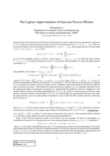
The Laplace Approximation of Gaussian Process Mixture

The Laplace Approximation of Gaussian Process Mixture
Topic: Learning Algorithms
Preference: oral
Zhengdong Lu
Department of Computer Science and Engineering
OGI School of Science and Engineering , OHSU
{zhengdon}@csee.ogi.edu
Various models of Gaussian process mixture have been proposed, mainly to address the non-stationarity in regression
[1, 2, 3]. Typically, a Gaussian process mixture consists of M Gaussian processes F = {f1, f2, · · · , fM } with zero
mean and covariance function specified by parameters Θ = {θ1, θ2, · · · , θM }, and a gating network g. For any input
x, g(x) = [g1(x), g2(x), · · · , gM (x)] with
M
gm(x) ≥ 0, m = 1, 2, · · · , M and gm(x) = 1.
As in [1], the probability model is as follows. Given input X = {x1, x2, ..., xN}, we define the latent variable
Z = {z1, z2, ..., zN} to indicate which process each xi is involved in. The probability of Z, given the gating network
g and input X, is
N
N
P (Z|X, g) = P (zi|xi, g) = gzi(xi). (1)
i=1
The probability of the output Y = {y1, y2, ..., yN} is
P (Y |X, g, Θ) =
P (Y, Z|X, g, Θ) =
P (Y |X, Z, Θ)P (Z|X, g) (2)
Z
where P (Y |X, Z, Θ) = M m=1 P ({yi : zi = m}|{xi : zi = m}; θm). Here, P ({yi : zi = m}|{xi : zi = m}; θm) is
the Gaussian distribution of all the yi generated by fm according to Z. The Gaussian process mixture given in equation
(1)-(2) is suitable for situation where the domain consists of different regimes that should be described by different
types of Gaussian processes. Unfortunately the regression based on equation (1)-(2) is generally intractable due to
the exponential number of summations in equation (2). Traditionally this problem is solved by sampling [1]. Our
method, instead, considers the Laplace approximation of P (Y |X, g, Θ), which is a Gaussian process with zero mean
and the covariance function as the GP mixture P (Y |X, g, Θ). Interestingly, this approximation becomes exact when
the gating network g gives us a hard partition of domain [3]. Easy to show that the covariance function of Gaussian
process mixture is:
M
E(yiyj|xi, xj, g, Θ) = Km(xi, xj)P (zi = m, zj = m|xi, xj, g) (3)
m=1
where Km(xi, xj) is the covariance function associated with process fm. Using ˆ K(·, ·; g, Θ) to denote the covariance
function given in equation (3), our Laplace approximation of the likelihood of Y is PL(Y |X, ˆ 1
K) = √
2πN | KX ˆ +σ2I| exp(− 1
2y′ ( ˆ KX + σ2I) −1y), where σ2 is the variance of observation noise and ˆ KX is the covariance matrix evaluated
on X. We find a suitable gating network by maximizing the data likelihood PL.
Figure 1 and 2 show the regression results of our model on two toy examples. In these two experiments, we
considered the mixture of two Gaussian processes with covariance function of process fm, (m = 1, 2) specified as
Z
m=1
i=1
Km(xi, xj) = exp(−||xi − xj|| 2 /s 2 m), m = 1, 2
where sm is the width of the RBF kernel for the m th Gaussian process, which are chosen beforehand. We use the
same gating network used in [2] and fit it with gradient descent. We report the regression result given by the probability
PL(y|x, X, Y, Θ, ˆ K). As shown in the two figures, our model automatically finds the appropriate gating network and
yields regression result significantly better than the Gaussian process regression with either f1 or f2.
1

g 1
1.5
1
0.5
0
0 0.5 1
x
1.5 2
(a) Output of g1
y
1.5
1
0.5
0
−0.5
−1
2
K1:s =3
1
2
K2:s =0.05
2
fitted K
−1.5
0 0.5 1
x
1.5 2
(b) Regression result
Figure 1: The regression result.(b)Blue line: true curve. Blue stars: noisy observation. Black curve: f1, s 2 1 = 3 ; Red
curve: f2, s 2 2 = 0.05 ; Green curve: Laplace Approximation of mixture of {f1, f2} with fitted K.
g 1
1.5
1
0.5
0
0 0.5 1
x
1.5 2
(a) Output of g1
y
1.5
1
0.5
0
−0.5
−1
2
K1:s =0.5
1
2
K2:s =0.01
2
fitted K
−1.5
0 0.5 1
x
1.5 2
(b) Regression result
Figure 2: The regression result. (b) Blue line: truth. Blue stars: noisy observation. Black curve: f1, s 2 1 = 0.5 ; Red
curve: f2, s 2 2 = 0.01 ; Green curve: Laplace Approximation of mixture of {f1, f2} with fitted K.
References
[1] C. Rasmussen and Z. Ghahramani. Infinite mixtures of gaussian process experts. In NIPS 14, 2002.
[2] V. Tresp. Mixtures of gaussian processes. In NIPS 13, 2001.
[3] O. Walliams. A Switched Gaussian Process for Estimating Disparity and Segmentation in Binocular Stereo. In
NIPS 19, 2007.
2