Implementing a Fast Cartesian-Polar Matrix Interpolator - MIT

Implementing a Fast Cartesian-Polar Matrix
Interpolator
Abhinav Agarwal, Nirav Dave, Kermin Fleming, Asif Khan,
Myron King, Man Cheuk Ng, Muralidaran Vijayaraghavan
Computer Science and Artificial Intelligence Lab
Massachusetts Institute of Technology
Cambridge, Massachusetts 02139
Email: {abhiag, ndave, kfleming, aik, mdk, mcn02, vmurali}@csail.mit.edu
Abstract—The 2009 MEMOCODE Hardware/Software Co-
Design Contest assignment was the implementation of a
cartesian-to-polar matrix interpolator. We discuss our hardware
and software design submissions.
I. INTRODUCTION
Each year, MEMOCODE holds a hardware/software codesign
contest, aimed at quickly generating fast and efficient
implementations for a computationally intensive problem. In
this paper, we present our two submissions to the 2009
MEMOCODE hardware/software co-design contest: a pure
hardware cartesian-to-polar matrix interpolator implemented
on the XUP platform and a pure software version implemented
in C.
Microarchitectural tradeoffs are difficult to gauge even in
a well-understood problem space. To better characterize these
tradeoffs, researchers typically build simulation models early
in the design cycle. Unfortunately in our case, the tight contest
schedule precluded such studies. Worse, we had no prior
experience within the problem domain nor were we able to
find an existing body of research as in years past. As a result,
we relied on simplified mathematical analysis to guide our
microarchitectural decisions. In this paper we will discuss our
rationale and the resulting microarchitecture.
II. PROBLEM DESCRIPTION
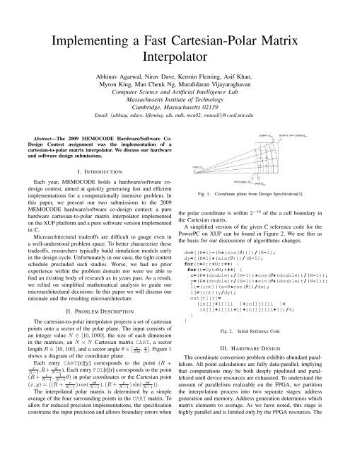
The cartesian-to-polar interpolator projects a set of cartesian
points onto a sector of the polar plane. The input consists of
an integer value N ∈ [10, 1000], the size of each dimension
in the matrices, an N × N Cartesian matrix CART, a sector
length R ∈ [10, 100], and a sector angle θ ∈ [ π π
256 , 4 ]. Figure 1
shows a diagram of the coordinate plane.
Each entry CART[x][y] corresponds to the point (R +
x
y
N−1 ,R+ N−1 ). Each entry POL[t][r] corresponds to the point
(R + r
N−1 , t
N−1 θ) in polar coordinates or the Cartesian point
(x, y) = ((R + r
tθ
r
tθ
N−1 ) cos( N−1 ), (R + N−1 ) sin( N−1 )).
The interpolated polar matrix is determined by a simple
average of the four surrounding points in the CART matrix. To
allow for reduced precision implementations, the specification
constrains the input precision and allows boundary errors when
Fig. 1. Coordinate plane from Design Specification[1]
the polar coordinate is within 2 −16 of the a cell boundary in
the Cartesian matrix.
A simplified version of the given C reference code for the
PowerPC on XUP can be found in Figure 2. We use this as
the basis for our discussions of algorithmic changes.
dx=((R+1)-(R*(cos(θ))))/(N-1);
dy=((R+1)*(sin(θ)))/(N-1);
for(r=0;r

memory stage uses the generated addresses to load the data,
performing a simple average and writing the result back to
memory. Like the first stage, this stage is completely dataparallel,
though it is constrained by the physical memory
bandwidth available on the FPGA board. Figure 3 shows the
top-level block diagram.
PowerPC
Address
Generation
System Memory
DMA Engine
Memory
Subsystem
Fig. 3. Top-Level Diagram
There is no advantage to over-engineering either stage of
the pipeline, since, by Little’s law, unbalancing the pipeline
throughput buys no performance. However, determining the
correct balance of resources allocated to the pipeline stages
is non-trivial. A priori, it is difficult to estimate the resources
required to produce addresses at a certain rate. Instead, We
will analyze the memory system, since it is constrained by
the maximum speed of the off-chip memory. We reused the
PLB-Master DMA Engine [2] built for a previous contest
submission, which transfers an average of one 32-bit word
per cycle when running in burst mode. Each coordinate
computation requires four 32-bit reads and one 32-bit write.
Thus, to process one polar coordinate per cycle, we require
an effective bandwidth five times greater than our physical
memory bandwidth. Even with good cache organization, this
bandwidth will be difficult to sustain. We therefore cap the
address generation performance at a single address request
per cycle and allocate all remaining resources to the memory
system.
A. Address Generation
For performance, we must frame the address generation
problem in such a way so as to exploit cache locality, while
minimizing resource consumption to permit higher performance
cache designs. To achieve these goals, we process the
polar coordinates in ray-major order. As rays are linear, we
can compute the fixed delta between adjacent points on a ray,
reducing multiplication to addition. This ordering also exhibits
good temporal and spatial locality of memory addresses. Adjacent
entries in the polar matrix are close together, sometimes
even aliasing to the same memory location. Figure 4 shows
the new algorithm.
This algorithm leaves only simple additions in the inner
loop. It also moves all division into initialization, allowing a
slow and simple hardware divider to be used. To avoid the
inv_dx= 1 / ((R+1)-(R*cos(θ)));
inv_dy= 1 / ((R+1)*sin(θ));
N1=N-1; theta = 0; dtheta = θ/N1;
rcost_dx = inv_dx * N1 * R * cos(θ);
for(t=0;t

(a) (b)
Fig. 5. Cache Behavior at Varying Ray Angles: Figure (a) shows an
example of a cache with 4-word burst size. Shaded blocks are needed for ray
computation, checked blocks are resident in the cache but will never be used
again. Figure (b) shows the π
case, in which all blocks in the cache are fully
4
utilized. The dark box in Figure (b) is a column.
Address Input
Second, coordinate interpolations touch two adjacent rows
in the cartesian matrix. This means we can partition odd and
even rows into separate caches, doubling cache bandwidth
without substantially increasing design complexity.
Third, address generation traverses the polar coordinates
in ray-major order, with monotonically increasing ray angles
to a maximum of π
4 . This monotonicity implies that if we
access a point in the cartesian matrix, we can guarantee that
no elements below that point in the matrix column will be
accessed in the future. Thus, assuming it is sufficiently large,
the cache will incur only cold misses, implying that no evicted
block will need to be re-fetched. This observation simplifies
the cache, since evicted blocks can be replaced as soon as the
new fill begins streaming in, without checking for write-afterread
(WAR) hazards.
This third observation merits some explanation, since an
insufficiently sized cache may still have WAR hazards. We
organize our cache logically as a set of small independent
caches which share tag-lookup and data store circuitry for
efficiency. Each small cache contains data from a particular
column of the cartesian array. The row size of each cache
and of each column is equal to the size of a memory burst.
Thus, conflicts may occur within the column but not between
columns. We achieve column independence by padding the
cartesian array in memory and providing sufficient cache area
for the number of columns in the largest permitted input. With
this cache organization and the maximum specified ray angle
of π
4 , we observe that if the column caches have capacity
equal to burst size plus one rows, we can avoid all capacity
and conflict misses and thus all WAR hazards. Figure 5 gives
a graphical demonstration of this claim. As the ray sweeps up,
only a set of trailing rows in each column will be used. Only
in the case of a ray angle of π
Data Output
Fig. 6. Cache Pipeline
tag match in the next stage. Tag hits are sent immediately to
the data access backend. Tag misses require an extra cycle
to emit a fill request and to update the tag bank. Since, by
construction, there are no hazards within the cache, we can
completely decouple the tag match from the data access to
improve performance. We give the tag match engine ample
buffering to allow many concurrent outstanding fill requests.
The data backend consists of two stages: data address and
data read, based on the read stages of the underlying BRAM
memories. Data is organized into two BRAM banks, allowing
unaligned requests to be satisfied in a single cycle.
The odd and even caches are connected to the DMA
engine via a round-robin arbiter. This organization gives us a
maximum effective memory bandwidth of 128 bits per cycle.
C. Testing
4 will each row in each column
cache contain live data. We can generate caches supporting
burst sizes up to 32 words on the XUP board.
1) The Cache Implementation: Based on these observations,
we developed a simple four stage pipeline, shown in
Figure 6. Logically, the pipeline can be divided into two parts:
Due to the large input space specified in the problem
description, verification by simulation of even a few large
scenarios was difficult. Since a full system operating on the
FPGA was implemented relatively quickly, we instead chose
to verify our implementation exclusively on the XUP board,
comparing the output against the reference software supplied
by the contest organizers. Unfortunately, for large tests, we
discovered that the reference software was prohibitively slow,
requiring hours to complete a single interpolation.
To ameliorate this situation, we applied a series of transformations,
inspired by our hardware design, to the reference
software. These optimizations, in turn, required us to verify
the modified software against the reference solution. However,
since only software needed to be verified, a much faster
general purpose machine could be used.
IV. SOFTWARE IMPLEMENTATION
tag match and data access.
During the verification of our accelerated software algo-
Tag matching starts with tag bank lookup, followed by a rithm, it became clear that the software, on a fast multicore,
External Memory
= =
Tag
Control
Tag Lookup
Tag Check
Data Request
Data Resp

outperformed the hardware implementation. We attribute this
difference to the superior memory systems of modern general
purpose processors.
A. Improving the Algorithm
As in hardware, using fixed point values for computation
resulted in a substantial speedup. To further improve performance,
we need to reduce the number of trigonometric functions.
This is accomplished by leveraging the sum-to-product
formulas for cosine and sine to derive a fast computation for
generating the sine-cosine pair for one ray from the sine-cosine
pair of the previous ray.
cos(θ + ∆θ) = cos(θ) cos(∆θ) − sin(θ) sin(∆θ)
sin(θ + ∆θ) = sin(θ) cos(∆θ) + sin(θ) cos(∆θ)
Since we scale cosine and sine by dx and dy we need to
rescale sin(∆θ) by dy
dx to obtain the correct results. Our final
single-threaded version can be found in Figure 7.
N1=N-1; RN=R*N1;
dx=((R+1)-(R*cos(theta)))/N1;
dy=((R+1)*sin(theta))/N1;
xoffset=R*cos(theta)/dx;
sin_dt_dy_dx=sin(theta/N1)*dy/dx;
sin_dt_dx_dy=sin(theta/N1)*dx/dy;
cos_dt=cos(theta/N1);
scaledcos_t=(1.0/(R+1 - (R*cos(theta));
scaledsin_t=0.0;
for(t=0;t