Problem Set 1 - Computation Structures Group - MIT
Problem Set 1 - Computation Structures Group - MIT
Problem Set 1 - Computation Structures Group - MIT

Create successful ePaper yourself
Turn your PDF publications into a flip-book with our unique Google optimized e-Paper software.
Massachusetts Institute of Technology<br />
Department of Electrical Engineering and Computer Science<br />
6.827 Multithreaded Parallelism: Languages and Compilers<br />
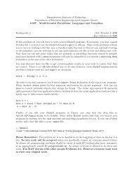
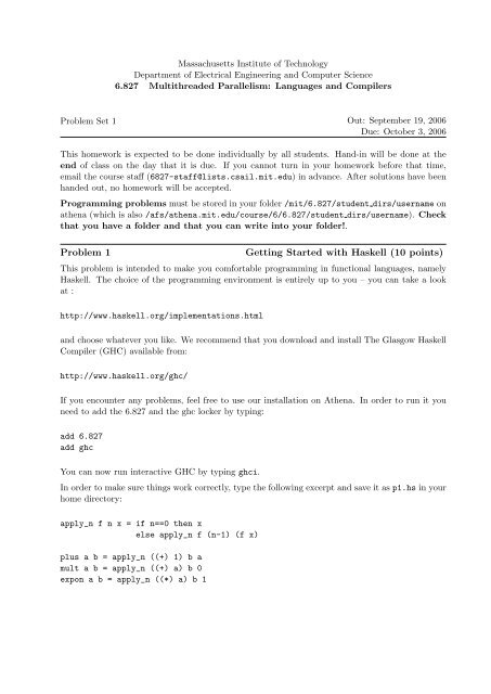
<strong>Problem</strong> <strong>Set</strong> 1 Out: September 19, 2006<br />
Due: October 3, 2006<br />
This homework is expected to be done individually by all students. Hand-in will be done at the<br />
end of class on the day that it is due. If you cannot turn in your homework before that time,<br />
email the course staff (6827-staff@lists.csail.mit.edu) in advance. After solutions have been<br />
handed out, no homework will be accepted.<br />
Programming problems must be stored in your folder /mit/6.827/student dirs/username on<br />
athena (which is also /afs/athena.mit.edu/course/6/6.827/student dirs/username). Check<br />
that you have a folder and that you can write into your folder!.<br />
<strong>Problem</strong> 1 Getting Started with Haskell (10 points)<br />
This problem is intended to make you comfortable programming in functional languages, namely<br />
Haskell. The choice of the programming environment is entirely up to you – you can take a look<br />
at :<br />
http://www.haskell.org/implementations.html<br />
and choose whatever you like. We recommend that you download and install The Glasgow Haskell<br />
Compiler (GHC) available from:<br />
http://www.haskell.org/ghc/<br />
If you encounter any problems, feel free to use our installation on Athena. In order to run it you<br />
need to add the 6.827 and the ghc locker by typing:<br />
add 6.827<br />
add ghc<br />
You can now run interactive GHC by typing ghci.<br />
In order to make sure things work correctly, type the following excerpt and save it as p1.hs in your<br />
home directory:<br />
apply_n f n x = if n==0 then x<br />
else apply_n f (n-1) (f x)<br />
plus a b = apply_n ((+) 1) b a<br />
mult a b = apply_n ((+) a) b 0<br />
expon a b = apply_n ((*) a) b 1
2 6.827 <strong>Problem</strong> <strong>Set</strong> 1<br />
then run ghci and load the file by typing:<br />
:l p1.hs<br />
Once you’ve loaded a file you can reload the file after you’ve changed it on disk with the command:<br />
:r<br />
You can now call one of the functions you have just specified by typing:<br />
expon 3 4<br />
(You should obtain 81).<br />
Now, back to the problem set.<br />
<strong>Problem</strong> 2 Simple Functions (25 points)<br />
In this problem, we examine two simple algorithms for numerical integration based on Simpson’s<br />
rule.<br />
Part a: (10 points)<br />
Given a function f and an interval [a, b], Simpson’s rule says that the integral can be approximated<br />
as follows:<br />
where<br />
I = h<br />
[f(a) + 4f(a + h) + f(a + 2h)]<br />
3<br />
h =<br />
b − a<br />
2<br />
For better accuracy, the interval of integration [a, b] is divided into several smaller subintervals.<br />
Simpson’s rule is applied to each of the subintervals and the results are added to give the total<br />
integral. If the subintervals of [a, b] are all of the same size p, where p = 2h, then we have the<br />
Composite Strategy for integration.<br />
Write a Haskell program containing a function<br />
composite_strategy f a b n<br />
where<br />
f is the function to integrate<br />
a, b are the endpoints of the integration interval
6.827 <strong>Problem</strong> <strong>Set</strong> 1 3<br />
n is the number of subintervals such that h = (b − a)/2n<br />
Integrate some simple functions and try different values for n.<br />
Part b: (10 points)<br />
If the subintervals of the integration are not all equal and can be changed as required, then we obtain<br />
an Adaptive Strategy for integration. A simple adaptive integration algorithm can be described as<br />
follows:<br />
1. Approximate the integral using Simpson’s rule over the entire interval [a, b]. Call this approximation<br />
old approx.<br />
2. Compute the midpoint x of the interval: x = (b + a)/2.<br />
3. Approximate a new interval by applying Simpson’s rule to the subintervals [a, x] and [x, b]<br />
and add the two results. Call this approximation new approx.<br />
4. If the absolute value of the difference between new approx and old approx is within some limit<br />
sigma then return new approx.<br />
5. Otherwise, apply the adaptive strategy recursively to each of the subintervals, add the two<br />
results, and return the sum as the answer.<br />
Write a Haskell program that contains the function<br />
adaptive_strategy f a b sigma<br />
Make sure adaptive strategy takes advantage of the parallelism available in the algorithm. Try<br />
integrating several functions while varying the sigma parameter.<br />
Part c: (5 points)<br />
How do the algorithms vary in complexity? Compare the accuracy of the answers. What factors<br />
affect the execution time and efficiency of the two strategies?<br />
<strong>Problem</strong> 3 Functions (25 points)<br />
In this problem we are going to generate a “<strong>Set</strong> of Integers” type. We will encode the set as a<br />
decider for membership in the set. For this problem programming is not necessary, and a writeup<br />
will suffice.<br />
type Int<strong>Set</strong> = (Int -> Bool)<br />
isMember :: Int<strong>Set</strong> -> Int -> Bool<br />
isMember f x = f x
4 6.827 <strong>Problem</strong> <strong>Set</strong> 1<br />
Part a: Simple <strong>Set</strong>s (2 points)<br />
Define the Empty set (the set with no elements) and the set of integers (contains all elements).<br />
empty<strong>Set</strong> :: Int<strong>Set</strong><br />
empty<strong>Set</strong> x = ...<br />
allInts :: Int<strong>Set</strong><br />
allInts x = ...<br />
Part b: Intervals (3 points)<br />
Write the function:<br />
-- interval x y contains all the integers in [x,y]<br />
interval :: Int -> Int -> Int<strong>Set</strong><br />
interval lBound uBound = ...<br />
Part c: More Interesting <strong>Set</strong>s (5 points)<br />
Generate a set of squares squares, which contains exactly all square numbers.<br />
Part d: <strong>Set</strong> Operators (10 points)<br />
Now that you can generate some sets, you need to generate operators to combine sets.<br />
Write the following functions:<br />
-- Boolean Operators<br />
setIntersection :: Int<strong>Set</strong> -> Int<strong>Set</strong> -> Int<strong>Set</strong><br />
setUnion :: Int<strong>Set</strong> -> Int<strong>Set</strong> -> Int<strong>Set</strong><br />
setComplement :: Int<strong>Set</strong> -> Int<strong>Set</strong><br />
-- <strong>Set</strong> generation<br />
addTo<strong>Set</strong> :: Int -> Int<strong>Set</strong> -> Int<strong>Set</strong><br />
deleteFrom<strong>Set</strong> :: Int -> Int<strong>Set</strong> -> Int<strong>Set</strong><br />
Part e: Equality (5 points)<br />
How would we define the equality operator on Int<strong>Set</strong>s? Would we be able to do better if we had<br />
used a list of Ints instead of a function to represent our set? What would we have had to give up<br />
to do that?
6.827 <strong>Problem</strong> <strong>Set</strong> 1 5<br />
<strong>Problem</strong> 4 Using λ combinators (25 points)<br />
The next two problems on this problem set focus on the pure λ-calculus. We recommend that you<br />
take a look at the pH Book, Appendix A, before you move on with this problem set. The idea is<br />
to become comfortable with the reduction rules used, and with the important differences between<br />
some of the reduction strategies which can be used when applying those rules.<br />
In this problem, we shall write a few combinators in the pure λ-calculus to get familiar with the<br />
rules of λ-calculus. Here are the definitions of some useful combinators.<br />
TRUE = λx.λy.x<br />
FALSE = λx.λy.y<br />
COND = λx.λy.λz.x y z<br />
FST = λf.f TRUE<br />
SND = λf.f FALSE<br />
PAIR = λx.λy.λf.f x y<br />
n = λf.λx.(f n x)<br />
SUC = λn.λa.λb.a (n a b)<br />
PLUS = λm.λn.m SUC n<br />
MUL = λm.λn.m (PLUS n) 0<br />
Now, write the λ-terms corresponding to the following functions.<br />
• (3 points) The boolean AND function.<br />
• (3 points) The boolean OR function.<br />
• (3 points) The boolean NOT function.<br />
• (6 points) The exponentiation function (EXP). You should write two expressions, one using<br />
MUL and the other without MUL (note: don’t eliminate MUL by substituting the body of<br />
the MUL combinator into your first definition—MUL only “stands for” its definition in the<br />
first place, so you’ve done nothing).<br />
• (5 points) The function ONE? which tests whether the given number is 1. (Hint: use the<br />
data structure combinators. Don’t try to construct a lambda term from whole cloth.)<br />
• (5 points) The function PRED which subtracts 1 from the given number. You may decide<br />
what to do when 0 is passed as an argument to PRED. (Extra credit: can you come up with<br />
a term T for which (SUC T) reduces to 0? If so, give the term; if not, explain why.)<br />
In addition to the given combinators, you are free to define any others which you think would be<br />
useful.<br />
<strong>Problem</strong> 5 Normal Order NF Interpreter for the λ calculus (50 points)<br />
In lecture, we discussed interpreters for the λ calculus, and gave two examples: call-by-name,<br />
written cn(E), and call-by-value, written cv(E). We consider both of these interpreters to terminate
6 6.827 <strong>Problem</strong> <strong>Set</strong> 1<br />
when they return an answer in Weak Head Normal Form. In this problem, we’re going to look<br />
at similar interpreters which yield answers in β normal form—that is, an expression which cannot<br />
possibly be β-reduced anymore.<br />
Part a: Step-wise Reduction (4 points)<br />
Consider the following term:<br />
(λx.λy.x)(λz.(λx.λy.x)z((λx.zx)(λx.zx)))<br />
Provide the first 2 reduction steps each for normal order and applicative order strategies.<br />
Remember, in normal order we pursue a leftmost redex strategy (choose the leftmost redex).<br />
In applicative order we pursue a leftmost innermost strategy (choose the leftmost redex, or the<br />
innermost such redex if the leftmost redex contains a redex).<br />
Part b: A Normal Order Interpreter (10 points)<br />
In the style presented in class, write an normal order interpreter. Remember we’re evaluating to<br />
normal form not weak head normal form.<br />
Now we’re going to code this interpreter up in Haskell.<br />
Part c: Renaming Function in Haskell (10 points)<br />
An expression will be of the form:<br />
data Expr =<br />
Var Name -- a variable<br />
| App Expr Expr -- application<br />
| Lambda Name Expr -- lambda abstraction<br />
deriving<br />
(Eq,Show) -- use default compiler generated Eq and Show instances<br />
type Name = String -- a variable name<br />
As a first step, write the function replaceVar :: (Name, Expr) -> Expr -> Expr which given a<br />
variable name x and a corresponding expression e, and an expression in which to do the replacement<br />
E, replaces all free instances of the variable x with the given expression e.<br />
Part d: Doing a Single Step (15 points)<br />
Now let’s write a function to do a single step of the reduction.<br />
Your normal order reduction will have the form: normNF OneStep :: ([Name],Expr) -> Maybe<br />
([Name],Expr). The Maybe type is defined in the prelude as:
6.827 <strong>Problem</strong> <strong>Set</strong> 1 7<br />
data (Maybe a) =<br />
Nothing<br />
| Just a<br />
normNF OneStep takes a list of fresh names, and a lambda expression. If there is a redex reduction<br />
available, it will pick the correct normal order redex and reduces it (possibly using the given fresh<br />
names for renaming). If a reduction was performed resulting in expr’ and reducing the names list<br />
to names’ the function returns Just (names’ expr’). Otherwise it will return the value Nothing.<br />
Part e: Repetition (3 points)<br />
Now write a function: normNF n :: Int -> ([Name],Expr) -> ([Name],Expr) which given an<br />
interger n, and an expression does n redex reductions (or as many as were possible) and returns<br />
the result (and the unused names).<br />
Part f: Generating New Names (4 points)<br />
Now we need a way to generate fresh variables names for an expression. Writing generating a list of<br />
variable names is simple leveraging the infinite list of positive integers [1..]. Use this to generate<br />
an infinite list of fresh names called freshNames.<br />
Remember, we want fresh variables and it is possible that our “fresh” names aren’t really fresh.<br />
What we need to do is make sure the ones we choose are not already used in the Expr.<br />
Write a function usedNames :: Expr -> [Name] which given an expression returns all the names<br />
used in it.<br />
Part g: Finishing Up (4 points)<br />
Then using these functions write normNF :: Int -> Expr -> Expr which given an integer n and<br />
an expression does n reductions to it and returns the result.