Information Sharing in a Multi-Echelon Inventory System
Information Sharing in a Multi-Echelon Inventory System
Information Sharing in a Multi-Echelon Inventory System
Create successful ePaper yourself
Turn your PDF publications into a flip-book with our unique Google optimized e-Paper software.
ZHAO Xiaobo (赵晓波) et al:<strong>Information</strong> <strong>Shar<strong>in</strong>g</strong> <strong>in</strong> a <strong>Multi</strong>-<strong>Echelon</strong>… 469<br />
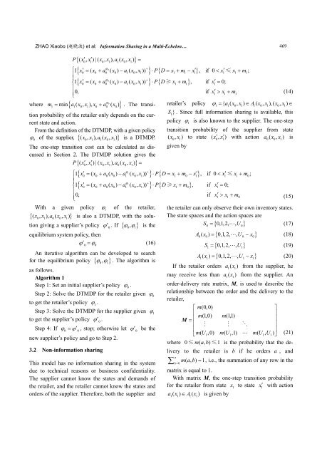
{ ( ′ ′ ) ( ) ( ) }<br />
P x0, x1 | x0, x1 , a1 x0, x1<br />
=<br />
ϕ0<br />
+<br />
⎧ 1 { x′ 0 = ( x0 + a0 ( x0) − a1( x0, x1)) } ⋅ P{ D = x1 + m1 − x′ 1} ,<br />
⎪<br />
ϕ0<br />
+<br />
⎨1<br />
{ x′ 0 = ( x0 + a0 ( x0) − a1( x0, x1)) } ⋅ P{ D≥x1 + m1} ,<br />
⎪<br />
⎪⎩<br />
0, if 0 < x′ 1≤x1 + m1;<br />
if x′<br />
1 = 0;<br />
if x′ 1 > x1 + m1<br />
(14)<br />
m = m<strong>in</strong> a ( x , x ) , x<br />
ϕ0<br />
+ a ( x ) . The transi- retailer’s policy ϕ 1 = { a1( x0, x1) ∈ A1( x0, x1) , ( x0, x1)<br />
∈<br />
where 1 { 1 0 1 0 0 0 }<br />
tion probability of the retailer only depends on the current<br />
state and action.<br />
From the def<strong>in</strong>ition of the DTMDP, with a given policy<br />
ϕ 0 of the supplier, { ( x0, x1) , a1( x0, x1)<br />
} is a DTMDP.<br />
The one-step transition cost can be calculated as discussed<br />
<strong>in</strong> Section 2. The DTMDP solution gives the<br />
P ( x′ , x′ ) | ( x , x ) , a ( x , x ) =<br />
{ }<br />
0 1 0 1 0 0 1<br />
{ ϕ1<br />
+ } { }<br />
{ ϕ1<br />
+ } { ≥ }<br />
1 } S . S<strong>in</strong>ce full <strong>in</strong>formation shar<strong>in</strong>g is available, this<br />
policy ϕ 1 is also known to the supplier. The one-step<br />
transition probability of the supplier from state<br />
( x0, x1)<br />
to state ( x′ 0, x′<br />
1)<br />
with action a0( x0, x1)<br />
is<br />
given by<br />
⎧ 1 x′ 0 = ( x0 + a0( x0) − a1 ( x0, x1)) ⋅ P D = x1 + m0 − x′ 1 , if 0 < x′ 1≤x1 + m0;<br />
⎪<br />
⎨1<br />
x′ 0 = ( x0 + a0( x0) − a1 ( x0, x1)) ⋅ P D x1 + m0 , if x′<br />
1 = 0;<br />
⎪<br />
⎪⎩<br />
0, if x′ 1 > x1 + m0<br />
With a given policy ϕ 1 of the retailer,<br />
{ ( x x ) a ( x x ) }<br />
0, 1 , 0 0, 1 is also a DTMDP, with the solution<br />
giv<strong>in</strong>g a supplier’s policy ϕ′ 0 . If { ϕ0, ϕ1}<br />
is the<br />
equilibrium system policy, then<br />
ϕ ϕ′ = (16)<br />
0<br />
An iterative algorithm can be developed to search<br />
for the equilibrium policy { ϕ0, ϕ1}<br />
. The algorithm is<br />
as follows.<br />
Algorithm 1<br />
Step 1: Set an <strong>in</strong>itial supplier’s policy ϕ 0 .<br />
Step 2: Solve the DTMDP for the retailer given ϕ 0<br />
to get the retailer’s policy ϕ 1 .<br />
Step 3: Solve the DTMDP for the supplier given ϕ 1<br />
to get the supplier’s policy ϕ′ 0 .<br />
Step 4: If ϕ0 = ϕ′ 0 , stop; otherwise let ϕ′ 0 be the<br />
new supplier’s policy and go to Step 2.<br />
3.2 Non-<strong>in</strong>formation shar<strong>in</strong>g<br />
This model has no <strong>in</strong>formation shar<strong>in</strong>g <strong>in</strong> the system<br />
due to technical reasons or bus<strong>in</strong>ess confidentiality.<br />
The supplier cannot know the states and demands of<br />
the retailer, and the retailer cannot know the states and<br />
orders of the supplier. Therefore, both the supplier and<br />
0<br />
(15)<br />
the retailer can only observe their own <strong>in</strong>ventory states.<br />
The state spaces and the action spaces are<br />
S = 012 , , , , U<br />
(17)<br />
{ }<br />
0 0<br />
{ }<br />
A ( x ) = 01 , , 2,<br />
, U −x<br />
(18)<br />
0 0 0 0<br />
{ 012 }<br />
S = ,, , , U<br />
(19)<br />
1 1<br />
{ }<br />
A1( x1) = 0,1,2, , U1 −x1<br />
(20)<br />
If the retailer orders a1( x 1)<br />
from the supplier, he<br />
may receive less than a1( x 1)<br />
from the supplier. An<br />
order-delivery rate matrix, M, is used to describe the<br />
relationship between the order and the delivery to the<br />
retailer,<br />
⎡ m(0,<br />
0)<br />
⎤<br />
⎢<br />
m(1,0) m(1,1)<br />
⎥<br />
M = ⎢ ⎥<br />
⎢ ⎥<br />
⎢ ⎥<br />
⎣mU ( 1, 0) mU ( 1,1) mU ( 1, U1)<br />
⎦ (21)<br />
where 0 ≤mab ( , ) ≤ 1 is the probability that the delivery<br />
to the retailer is b if he orders a , and<br />
a<br />
( , ) 1<br />
b 0<br />
mab ∑ = , i.e., the summation of any row <strong>in</strong> the<br />
=<br />
matrix is equal to 1.<br />
With matrix M, the one-step transition probability<br />
for the retailer from state x 1 to state x′ 1 with action<br />
a ( x ) ∈ A( x ) is given by<br />
1 1 1 1


