Parameter Uncertainty in CGE Modeling of the Macroeconomic Impact

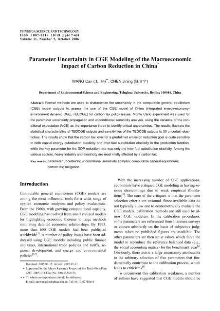
TSINGHUA SCIENCE AND TECHNOLOGY
ISSN 1007-0214 18/18 pp617-624
Volume 11, Number 5, October 2006
Parameter Uncertainty in CGE Modeling of the Macroeconomic
Impact of Carbon Reduction in China *
WANG Can (王 灿) ** , CHEN Jining (陈吉宁)
Department of Environmental Science and Engineering, Tsinghua University, Beijing 100084, China
Abstract: Formal methods are used to characterize the uncertainty in the computable general equilibrium
(CGE) model outputs to assess the use of the CGE model of China (integrated energy-economy-
environment dynamic CGE, TEDCGE) for carbon tax policy issues. Monte Carlo experiment was used for
the parameter uncertainty propagation and unconditional sensitivity analysis, using the variance of the con-
ditional expectation (VCE) as the importance index to identify critical uncertainties. The results illustrate the
statistical characteristics of TEDCGE outputs and sensitivities of the TEDCGE outputs to 50 uncertain elas-
ticities. The results show that the carbon tax level for a predefined emission reduction goal is quite sensitive
to both capital-energy substitution elasticity and inter-fuel substitution elasticity in the production function,
while the key parameter for the GDP reduction rate was only the inter-fuel substitution elasticity. Among the
various sectors, heavy industry and electricity are most vitally affected by a carbon tax.
Key words: parameter uncertainty; unconditional sensitivity analysis; computable general equilibrium;
Introduction
carbon tax; mitigation
Computable general equilibrium (CGE) models are
among the most influential tools for a wide range of
applied economic analyses and policy evaluations.
From the 1960s, with growing computational capacity,
CGE modeling has evolved from small stylized models
for highlighting economic theories to large methods
simulating detailed economic relationships. By 1995,
more than 600 CGE models had been published
worldwide [1] . A number of policy issues have been addressed
using CGE models including public finance
and taxes, international trade policies and tariffs, regional
development, and energy and environmental
policies [2-7] .
*
**
Received: 2005-04-15; revised: 2005-07-11
Supported by the Major Research Project of the Tenth Five-Plan
(2001-2005) of China (No. 2004-BA611B)
To whom correspondence should be addressed.
E-mail: canwang@tsinghua.edu.cn; Tel: 86-10-62785610
With the increasing number of CGE applications,
economists have critiqued CGE modeling as having serious
shortcomings due to weak empirical foundations
[8] . The core of the critiques is that the parameter
selection criteria are unsound. Since available data do
not typically allow one to econometrically evaluate the
CGE models, calibration methods are still used by almost
CGE modelers. In the calibration procedures,
some parameters are referenced from literature surveys
or chosen arbitrarily on the basis of subjective judgments
when no published figures are available. The
other parameters are then set at values which force the
model to reproduce the reference balanced data (e.g.,
the social accounting matrix) for the benchmark year [2] .
Obviously, there exists a large uncertainty attributable
to the arbitrary selection of free parameters that fundamentally
contribute to the calibration process, which
leads to criticisms [8] .
To circumvent this calibration weakness, a number
of authors have suggested that CGE models should be

618
tested for robustness by implementing sensitivity
analyses around the elasticity mean values [9-14] . However,
in practice most analyses use limited sensitivity
analyses, with changes in a few key elasticities to examine
the sensitivity of the results. This procedure has
no way of ensuring that the chosen elasticities are the
important ones, and its role is also limited by the discretionary
character of the values selected. Few of the
existing studies either systematically explore the parameter
uncertainty propagation or examine the contribution
of the various parameters to the uncertainty due
to the expensive computing costs. Harrison et al. [11]
and Alber et al. [13] conducted unconditional sensitivity
analyses, but they focused only on some of the elasticities
and failed to describe the CGE output distributional
information.
The purpose of this paper is to study the problem of
measuring the uncertainty of CGE model simulations
associated with parameter uncertainty using the macroeconomic
impacts of a carbon tax in China as the
policy question for the simulations. The study used
Monte Carlo experiments for the parameter uncertainty
propagation and employed an unconditional systematic
sensitivity analysis procedure to identify critically sensitive
elasticities. The analytical process adopted in this
paper is extensively used in model evaluations [15] .
1 CGE Model
The model developed here, integrated energyeconomy-environment
dynamic CGE (TEDCGE), is a
time recursive dynamic general equilibrium model,
which has been presented in detail [16] . Since the dynamic
mechanism has little impact on the elasticities’
influence on the CGE output and it is very time consuming
compared with the static CGE model, the static
version of the model was used to examine the elasticities’
uncertainties.
The TEDCGE model provides a description of the
China economy of 1997, the latest year for which the
China input/output is available. The model identifies
10 production sectors (agriculture, heavy industry,
light industry, transportation, construction, service
electricity, coal, oil, and natural gas, which are numbered
as 1 to 10, respectively), 10 consumption goods,
and 2 household groups distinguished by rural and urban
residents. The model operates by simulating the
operation of markets for factors, products, and foreign
Tsinghua Science and Technology, October 2006, 11(5): 617-624
exchange. The model is highly nonlinear, with equations
specifying supply and demand behavior across all
markets. The model pays particular attention to modeling
the energy sector and its linkages to the rest of the
economy. The energy use is disaggregated into coal, oil,
natural gas, and electricity in the model. Along with
capital, labour, and intermediate inputs, the four energy
inputs are regarded as the basic inputs into the production
function.
The carbon tax revenue from the sectoral energy
consumption is described by
E
10 10
∑∑
RC ( t) = tc ⋅ε⋅(1−fc ) ⋅θ ⋅VE ( t)
⋅ο
i= 1 j=
7
h= 1 j=
7
j j j ji j
(1)
The carbon tax revenue from residential energy use is
described by
2 10
RC C ( t) = ∑∑ tc ⋅εj ⋅θj ⋅CI hj( t)
⋅οj
(2)
VEji is the monetary consumption (RMB) of fuel j by
sector i, CIhj is the residential consumption (RMB) of
fuel j by household h, tc denotes the carbon tax rate in
terms of RMB/t, εj denotes the CO2 emission coefficient
of fuel j with the unit of t/TJ, fcj is the carbon
fixed rate of fuel j, θj is the conversion factor of fuel j
from a nominal output value to a physical term with the
unit of TJ/RMB, and οj is the oxidation rate of fuel j.
The CO2 emissions are calculated for each sector by
means of the sectoral fuel consumption and the corresponding
emission coefficient. Since the fuel consumption
is in terms of the corresponding nominal output
rather than directly as the physical units in the model,
the sectoral real fuel consumption is first translated
into physical terms, using a fuel-specific technical
conversion factor, and then further converted into CO2
based on the fuel-specific emission coefficient. The
fuel used by different sectors is assumed to have the
same quality, implying equivalent emission factors, in
terms of tons of CO2 per unit of fuel consumption, for
a fuel used in production, households, or government.
A carbon tax is incorporated into the model as a means
of achieving an assumed carbon reduction target. The
tax applies to the consumption of primary fuels only;
that is, the energy sectors only pay the carbon tax on
their own use of fuels. The carbon tax revenue is recycled
to the economy in several alternative ways, ensuring
that the total government revenue is neutral to the
carbon tax.

WANG Can (王 灿) et al:Parameter Uncertainty in CGE Modeling of… 619
As with most CGE models, the substitution elasticities
and the transformation elasticities are incorporated
through constant elasticity of substitution (CES)
and constant elasticity of transformation (CET) functions
into the production and import/export decisionmaking
procedure in TEDCGE. Both these functions
have the same general form:
( ( ) ) 1
ρ
−
1 1
2
ρ
Y = φ δ ⋅ X + −δ ⋅ X ρ (3)
where Y is the aggregate composite of X1 and X2, φ is
the efficiency parameter, δ is the share parameter, and
ρ is the substitution parameter. The substitution parameter
is a function of the substitution or transformation
elasticity, ε, defined as ρ = ( ε −1) ε if Eq. (3) is a
CES and as ρ = ( ε + 1) ε if Eq. (3) is a CET. The full
model includes, as exogenous parameters, four substitution
elasticities (three in the production function and
one in the import demand function) and one transformation
elasticity (in the export supply function) for
each of the ten sectors, for a total of 50 elasticities to
be defined in the calibration process.
2 Uncertainty Analysis Method
Monte Carlo simulations and unconditional systematic
sensitivity analysis were used to determine the uncertainty
in the CGE model results given the parameter
uncertainty and to determine the importance of each
individual parameter with respect to the uncertainty in
the outputs. These questions are answered through
quantification of the uncertainty in the screened parameters
in the form of prior probability distributions,
based on random parameter values and repeated model
simulations. Given a large number of simulations, the
probability distributions of the outcomes can be constructed
as a histogram of the outcomes that approximate
with arbitrarily small error the “true” probability
density function of the model outcomes.
Since all of the uncertain elasticities in question are
theoretically constrained to be at least non-negative
and non-infinite, the beta family of distributions was
chosen for its finite end-points and its flexibility in representing
different distribution shapes. A standard beta
distribution, which is defined over the interval (0, 1),
can be transformed to any desired scale through a simple
linear transformation. The beta distribution function
has two parameters a and b and is defined as
⎧ Γ ( a+ b) a−1 b−1
⎪ x (1 − x) , 0 < x<
1;
f( x/ a, b)
= ⎨Γ( a) Γ(
b)
⎪⎩ 0, o t h erwise
(4)
Different values for the two parameters a and b will
define various shapes and variances of the distribution.
For example, a and b are greater than or equal to 1 for
symmetric and unimodal beta distributions. The population
parameters of each elasticity’s distribution (e.g.,
the minimum and maximum end-points) are chosen on
the basis of empirical studies. The next section presents
detailed information describing uncertain elasticities
examined in this paper.
Once the ranges and distributions of elasticities have
been established, the next step is to determine an adequate
sampling intensity for the Monte Carlo experiment.
The sampling intensity is chosen to limit the
margins of error in the estimated means and variances
of the model’s output variables of interest to a prespecified
level, chosen to be 1% in this paper.
This approach quantifies the variations in the model
response, but the procedure cannot identify the driving
uncertainties, which are the uncertain parameters that
cause the most variance in the outputs of interest. An
unconditional sensitivity analysis, which focuses on
the output uncertainty over the entire range of values
of the input parameters, is the preferable procedure for
identifying the driving uncertainties. The unconditional
sensitivity analysis method was described by Saltelli et
al. [16] In this study, the 50 elasticities of substitution are
treated as uncertain and allowed to take random values
from their probability density functions. For each perturbation
of the elasticities, the TEDCGE model is recalibrated
and then solved for the benchmark and
counterfactual equilibria. The actual data generating
procedure for the calibration data set could be described
as follows:
For i = 1, 50 (50 elasticity parameters)
Define s i points that are the mean values of s i non-
overlapping intervals of equal probability, which are exhaus-
tively divided in the sampling space of parameter i
For j = 1, s i (fixed s i points of parameter i)
For n = 1, K (sampling intensity)
Select a random value from the beta distribution for
each of the 49 elasticity parameters besides parame-
ter i
Calibrate the model based on the 50 parameters

620
End
value and the benchmark year data
Run the model
Calculate the mean and variance of the model output
for the K runs
End
Calculate the importance measure of uncertain parameter i
(defined as the difference between the maximum and
minimum mean output value over its si points)
End
Rank the parameters by the value of their importance measure
All beta variates were generated based on a rejection-acceptance
algorithm (algorithm BS) [17] . The random
data matrix can either be generated using a crude
Monte Carlo algorithm or some form of stratified sampling,
such as Latin hypercube sampling (LHS). LHS
was used in this study to reduce the computation cost
using software developed in Visual Basic to call for the
execution of the general algebraic modeling system
(GAMS) solution of TEDCGE.
3 Data and Results
The model was calibrated to a set of data for China in
1997. The data was aggregated into three broad categories:
detailed economic accounts, which are ideally
maintained in the form of a social accounting matrix
(SAM); structural parameters; and some subsidiary
data. The National Bureau of Statistics of China
(NBSC) [18] discovered the income and expenditures for
each household category, the imports and exports for
Tsinghua Science and Technology, October 2006, 11(5): 617-624
each sector, the labor and capital under each of the
production sectors as well as their level of output, the
transformation matrix between industrial output and
consumer goods, the investments by sector, and government
revenues and expenditures. Before calibration,
a number of adjustments to the original input/output
(I/O) table were necessary with the SAM used to impose
a general equilibrium structure on the economy,
since many inconsistencies or “residuals” may exist in
the I/O table. In addition, the 50 elasticities of substitution
in the model were predefined based on literature
values before calibration.
3.1 Uncertainties in the input parameters
Statistical information for the probability density functions
for each parameter such as the mode (most likely
value), the endpoints (the 0.00 and 1.00 fractiles) and
the level of variance of each uncertain parameter were
derived from existing literature data. All the elasticity
parameters selected as uncertain in the model are
summarized in Table 1 with their means, endpoints,
standard deviations, and relative errors (defined as
standard deviation divided by the mean). Details on
how and where the information was obtained can be
found in Wang [16] . Note that the distributions shown
here are not meant to precisely capture accurate values
of the input uncertainties, but rather to demonstrate
how much variation in the outcomes can be caused by
conservative estimates of the input uncertainties.
Table 1 Mean and standard deviations of the uncertain parameters in the TEDCGE model
Parameters Mean
Lower
bound
Upper
bound
Standard
deviation
Relative
error (%)
Beta distribution parameter
a b
Eee 1.00 0.5 1.5 0.25 25 1.5 1.5
Eke 0.50 0.2 1.4 0.26 40 1.5 2.5
Ecl 0.55 0.2 0.9 0.18 32 1.5 1.5
Eid 1.50 0.1 4.0 0.73 42 2.5 3.5
Eed 2.50 0.1 4.0 0.73 31 3.5 2.5
Note: Eee, elasticity substitution between energies; Eke, elasticity substitution between capital and energy aggregate; Ecl, elasticity substitution be-
tween capital-energy aggregate and labor; Eid, elasticity substitution between imported goods and domestic production; Eed, elasticity transfer between
export supply and domestic demand.
Figures 1 and 2 give examples of the probability distributions
for Eid and Eed. The TEDCGE reference runs
(neglecting the uncertainties) used a nominal value of
1.5 for the elasticity of import substitution (Eid) and 2.5
for elasticity of export transfer (Eed) for all sectors. The
modes of the distributions were chosen to reproduce
the reference assumptions. Both of these elasticities
were assumed to have the same endpoints. The lowest

WANG Can (王 灿) et al:Parameter Uncertainty in CGE Modeling of… 621
endpoint was set at 0 and the highest was set at 4.0.
The resulting distribution for import substitution elasticity
was modeled by a beta distribution with parameters
a = 2.5 and b = 3.5, while the beta parameters for
export transfer elasticity were a = 3.5 and b = 2.5.
Fig. 1 Probability distribution for elasticity of import
substitution
Fig. 2 Probability distribution for elasticity of export
transfer
3.2 Uncertainty in the TEDCGE outputs
Figure 3 shows the probability distributions for carbon
tax rates required to achieve the carbon reduction goals
of 10%, 20%, 30%, and 40% compared with the BAU
scenario for 2010 in China. 5000 repetitions of the
Monte Carlo experiment were first used to formulate
the probability distributions. The Monte Carlo experiments
were then repeated to get another probability
distribution. The errors in the means and variances
from these two experiments were found to be less than
1%, which means that the 5000 Monte Carlo simulations
give sufficiently accurate results. The implications
of the uncertainties are important when evaluating
the performance of a carbon tax policy for a carbon
mitigation strategy, but even in the absence of a policy
the uncertainties in the carbon tax rates have implications
for interpreting results. What is often called a
marginal abatement cost curve for the international
carbon emission trading model is in fact only one series
of values from a series of distributions of possible
values, given the uncertain parameters existing in the
model. Policy analysis with models on carbon emission
trading should be viewed in this context.
Fig. 3 Probability distribution of carbon tax rate response
to carbon reduction rates
The mean (bold middle line), the 95% and 100%
confidence intervals, and the relative error for the marginal
abatement cost curve in 2010 for China calculated
by TEDCGE are illustrated in Fig. 4. The results
show increasing means and variances for the abatement
cost as the carbon reduction goal increases. In
addition, the relative error in the TEDCGE output is
much smaller than the error in the input parameters
(see Table 1).
Fig. 4 Marginal abatement cost curve with parameter
uncertainties
The results show that if the input parameter statistical
information is fully provided, the CGE model outputs
also exhibit statistical characteristics reflecting the
uncertainties transmitted from the inputs to the simulation
results. Although parameter uncertainties throw
doubt on the reliability of the CGE model simulation
results, the input uncertainties are reduced to some extent
through the CGE modeling procedure.

622
3.3 Unconditional sensitivity analysis results
One of the most important contributions of the uncertainty
analysis is the identification of the driving uncertainties,
the uncertain parameters that cause the
most variance in the outputs of interest. Figure 5 shows
the effects of perturbations of each elasticity parameter
in its space with random values of other elasticity
Tsinghua Science and Technology, October 2006, 11(5): 617-624
parameters selected from their probability density
functions. The carbon tax rate and GDP reduction rate
calculated by the model when assuming a counterfactual
CO2 emission reduction goal of 20% in 2010 were
selected as typical TEDCGE outputs in Figs. 5a and 5b.
Only the influential parameters are named in Fig. 5.
Fig. 5 Effects of perturbations of each elasticity parameter in its space with other elasticities randomized from their
probability density functions. Only the most important factors are named. See the notes with Table 2 for explanation of
the sector indicators.
For a model with 50 uncertain input parameters such
as TEDCGE, only a few factors are likely to have a
sizeable influence. Figure 5 demonstrates that the TED-
CGE model results are sensitive to only a few of the parameters
when the critical parameters of various endogenous
variables are varied. For example, the uncertainty
in the elasticity of substitution between capital
and energy in three sectors (Eke(2), Eke(6), and Eke(10))
and the elasticity of substitution between different energy
sources in two sectors (Eee(2) and Eee(10)) are the
primarily parameters influencing the variances in the
carbon tax rate corresponding to a specific carbon emission
reduction rate, while the key parameters for the
GDP reduction rate are only the elasticity of substitution
between the different energy sources in the heavy industry
and natural gas sectors (Eee(2) and Eee(10)).
A simple measure of importance of an input factor,
α, was defined based on the so-called variance of the
conditional expectation (VCE) of outcome. Assume
that we are interested in describing the importance of
an elasiticity parameter α in TEDCGE. The importance
of α with regard to the output uncertainty can be assessed
by considering the conditional probability distributions
of the TEDCGE outputs conditioned on α.
The importance of a parameter is assumed to be related
to how much it affects the model output. Intuitively,
parameter α is important if fixing its value substantially
reduces the (conditional) output variance relative
to the marginal output variance. Hence, the variance
ratio can be used as an appropriate measure of importance.
In this study, the magnitude of the VCE relative
to the total variance in the output is defined as importance
index:
IM
αi
( Y )
[ ]
( )
[ ]
Var ⎡ α E α ⎤ VCE α
=
⎣ ⎦
= (5)
Var Y Var Y
where Varα [E(Y|α)] is the variance of the conditional
expectation of the model output of Y, conditioned on α,
that is, the variability in E(Y|α) as α varies. In fact, this
index is termed the correlation ratio and had been studied
and applied by many investigators for sensitivity
analysis [19] . The unconditional systematic sensitivity
analysis results can be used to calculate the importance
index for each uncertain elasticity parameter. Table 2
lists the top ten elasticities with the largest and smallest
sensitiveness to the endogenous variables of the carbon
tax rate and GDP reduction rate.

WANG Can (王 灿) et al:Parameter Uncertainty in CGE Modeling of… 623
Table 2 Order of the sensitivities of elasticities to the CGE model outputs
Top ten sensitive elasticities Top ten insensitive elasticities
To carbon tax rate To GDP loss rate To carbon tax rate To GDP loss rate
Elasticity IMαi Elasticity IMαi Elasticity IMαi Elasticity IMαi
E ke(2) 0.36 E ee(2) 0.36 E id(5) 0.02 E ed(9) 0.02
E ee(2) 0.31 E ee(10) 0.19 E ee(5) 0.02 E ee(1) 0.02
E ke(10) 0.26 E ee(7) 0.10 E ke(4) 0.02 E ke(9) 0.02
E ke(6) 0.16 E ke(2) 0.09 E id(9) 0.02 E ed(1) 0.02
E ee(10) 0.12 E ke(10) 0.09 E ed(10) 0.02 E ed(7) 0.03
E ke(3) 0.11 E ee(6) 0.09 E ed(7) 0.03 E ed(4) 0.03
E cl(2) 0.10 E cl(7) 0.09 E ed(9) 0.03 E id(10) 0.03
E ee(6) 0.09 E ee(9) 0.09 E ee(1) 0.03 E cl(1) 0.04
E cl(10) 0.08 E id(4) 0.09 E ke(9) 0.03 E ee(4) 0.04
E ed(6) 0.08 E ed(6) 0.08 E ed(4) 0.03 E id(7) 0.04
Notes: Figures at the end of the code indicate the sector: 1, Agriculture; 2, Heavy industry; 3, Light industry; 4, Transportation; 5, Construction;
6, Service; 7, Electricity; 8, Coal; 9, Oil, and 10, Natural gas.
Table 2 shows that the most sensitive elasticity parameters
are generally Eke (elasticity substitution between
capital and energy aggregate) and Eee (elasticity
substitution between different energy sources). The
elasticity parameters in the international trade function
(i.e, Eed and Eid) have relatively weak effects on the
outputs as shown in the top ten insensitive elasticities
in Table 2. When considering sectoral elasticities, the
elasticity parameters in heavy industry (Sector 2), service
(Sector 6), and natural gas sector (Sector 10) are
the most significant contributors listed in the left side of
Table 2. That means the elasticities of these three sectors
cause the most variations in the outputs. The elasticities
in the agriculture, transportation, and oil production sectors
(Sectors 1, 4, and 9) have little influence on the output
as shown on the right side of Table 2.
4 Conclusions
Computable general equilibrium modeling has become
an effective technique for evaluating a wide range of
policy questions. While uncertainties about the input
values in a CGE model may limit the credibility of its
conclusions, relatively few applications have explicitly
treated the uncertainties. This paper describes formal
methods for assessing this type of uncertainties and illustrates
its use in a TEDCGE model applied to a carbon
tax policy issue. The method relies on building
probability density functions of the CGE model output
using crude Monte Carlo experiments. In contrast to
the traditional opinions, the results indicate that not
only can uncertainty in the CGE model be described
given full statistical information on the input parameters,
but that the uncertainties have important quantitative
and qualitative consequences. The input uncertainty
can be reduced to some extent through the CGE
modeling procedure. The results also indicate that the
CGE model results were sensitive to only some of the
parameters when the critical parameters for different
endogenous variables are varied. The carbon tax level
corresponding to a predefined carbon reduction rate in
TEDCGE, for example, was quite sensitive to both the
capital-energy substitution elasticity and the inter-fuel
substitution elasticity in the production sector, while
the key parameter affecting the GDP reduction rate
was only the inter-fuel substitution elasticity. The results
also show that the heavy industry and electricity
sectors are the most important sectors affecting the
carbon tax level.
Acknowledgements
The manuscript was mostly prepared during the first author’s
stay as a guest researcher at the Energy Project of International
Institute for Applied Systems Analysis (IIASA). The authors
gratefully acknowledge Dr. Leo Schrattenholzer, Dr. Leonardo
Barreto, and Dr. Ji Zou for their valuable comments.

624
References
[1] Cockburn J, Savard L, Decaluwé B. SAGE: A database of
studies using applied general equilibrium models. In: The
Sixth International CGE Modeling Conference University
of Waterloo. Waterloo, Ontario, Canada, October 26-28,
1995.
[2] Shoven J B, Whalley J. Applying General Equilibrium.
Cambridge: Carbridge University Press. 1992.
[3] Gunning J W, Keyzer M A. Applied general equilibrium
models for policy analysis. In: Behrman J, Srinivasan T,
eds. Handbook of Development Economics, vol. 3A. Amsterdam:
North-Holland, 1995: 2026-2107.
[4] Bhattacharyya S C. Applied general equilibrium models
for energy studies: A survey. Energy Economics, 1996,
18(3): 145-164.
[5] Evas B C, Schmedders K. General equilibrium models and
homotopy methods. Journal of Economic Dynamics and
Control, 1999, 23(10&11): 1249-1279.
[6] Devarajan S, Robinson S. The influence of computable
general equilibrium models on policy. In: Kehoe T J,
Srinivasan T N, Whalley J, eds. Frontiers in Applied General
Equilibrium Modeling. Cambridge: Cambridge University
Press, 2005: 402-428.
[7] Wang C, Chen J, Zou J. Impacts assessment of CO2 mitigation
to China’s economy based on a CGE model. Journal
of Tsinghua University (Science & Technology), 2005,
45(12): 1621-1624. (in Chinese)
[8] McKitrick R R. The econometric critique of computable
general equilibrium modeling: The role of functional
forms. Economic Modelling, 1998, 15 (14): 543-573.
[9] Pagan A R, Shannon J H. Sensitivity analysis for linearized
computable general equilibrium models. In: Piggot
J, Whalley J, eds. New Developments in Applied General
Equilibrium Analysis. Cambridge: Cambridge University
Press, 1985.
Tsinghua Science and Technology, October 2006, 11(5): 617-624
[10] Harrison G W, Vinod H D. The sensitivity analysis of applied
general equilibrium models completely randomized
factorial sampling designs. The Review of Economics and
Statistics, 1992, 74(2): 357-362.
[11] Harrison G W, Jones R, Kimbell L J, Wigle R. How robust
is applied general equilibrium analysis? Journal of Policy
Modelling, 1993, 15(1): 99-115.
[12] Canova F. Sensitivity analysis and model evaluation in
simulated dynamic general equilibrium economies. International
Economic Review, 1995, 36(2): 477-501.
[13] Abler D G, Rodríguez A G, Shortle J S. Parameter uncertainty
in CGE modeling of the environmental impacts of
economic policies. Environmental and Resource Economics,
1999, 14(2): 75-94.
[14] Bernow S, Cleetus R, Laitner J A, Peters I, Rudkevich A,
Ruth M. A pragmatic CGE model for assessing the influence
of model structure and assumptions in climate change
policy analysis. In: Kreiser L A, ed. Critical Issues in International
Environmental Taxation. Chicago: CCH
Incorporated, IL, 2002.
[15] Saltelli A, Chan K, Scott E M. Sensitivity Analysis. New
York: John Wiley & Sons, Ltd., 2000.
[16] Wang C. Climate change policy simulation and uncertainty
analysis: A dynamic CGE model of China [Dissertation].
Beijing: Tsinghua University, 2003. (in Chinese)
[17] Ahrens J H, Dieter U. Computer methods for sampling
from gamma, beta, poisson, and binomial distributions.
Computing, 1974, 12(3): 223-246.
[18] NBSC (National Bureau of Statistics of China). China’s
Input Output Table 1997. Beijing: Statistics Press of China,
1999. (in Chinese)
[19] McKay M D. Nonparametric variance-based methods of
assessing uncertainty importance. Reliability Engineering
and System Safety, 1997, 52(3): 267-279.