Fast extraction and rendering of isosurfaces from 4D data
Fast extraction and rendering of isosurfaces from 4D data
Fast extraction and rendering of isosurfaces from 4D data

You also want an ePaper? Increase the reach of your titles
YUMPU automatically turns print PDFs into web optimized ePapers that Google loves.
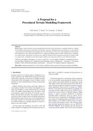
a) b) c)<br />
Figure 2: a) Intervals represented as points in Span Space. b) The intervals spanning a given isovalue Viso are<br />
located in the upper left corner <strong>from</strong> the point (Viso, Viso). c) The search for intervals spanning a given isovalue<br />
Viso is done in three steps, corresponding to three regions in Span Space.<br />
Tree consists <strong>of</strong> a balanced binary tree, whose nodes<br />
correspond to values <strong>of</strong> X, plus two lists <strong>of</strong> intervals<br />
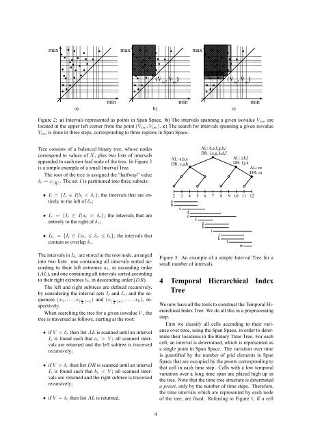
appended to each non-leaf node <strong>of</strong> the tree. In Figure 3<br />
is a simple example <strong>of</strong> a small Interval Tree.<br />
The root <strong>of</strong> the tree is assigned the “halfway” value<br />
δr = x h ⌈ 2 ⌉. The set I is partitioned into three subsets:<br />
• Il = {Ii ∈ I|bi < δr}; the intervals that are entirely<br />
to the left <strong>of</strong> δr;<br />
• Ir = {Ii ∈ I|ai > δr}; the intervals that are<br />
entirely to the right <strong>of</strong> δr;<br />
• Iδr = {Ii ∈ I|ai ≤ δr ≤ bi}; the intervals that<br />
contain or overlap δr.<br />
The intervals in Iδr are stored in the root node, arranged<br />
into two lists: one containing all intervals sorted according<br />
to their left extremes ai, in ascending order<br />
(AL), <strong>and</strong> one containing all intervals sorted according<br />
to their right extremes bi, in descending order (DR).<br />
The left <strong>and</strong> right subtrees are defined recursively,<br />
by considering the interval sets Il <strong>and</strong> Ir, <strong>and</strong> the se-<br />
quences (x1, . . . , x ⌈ h<br />
2 ⌉−1) <strong>and</strong> (x ⌈ h<br />
2 ⌉+1, . . . , xh), respectively.<br />
When searching the tree for a given isovalue V , the<br />
tree is traversed as follows, starting at the root:<br />
• if V < δr then list AL is scanned until an interval<br />
Ii is found such that ai > V ; all scanned intervals<br />
are returned <strong>and</strong> the left subtree is traversed<br />
recursively;<br />
• if V > δr then list DR is scanned until an interval<br />
Ii is found such that bi < V ; all scanned intervals<br />
are returned <strong>and</strong> the right subtree is traversed<br />
recursively;<br />
• if V = δr then list AL is returned.<br />
4<br />
Figure 3: An example <strong>of</strong> a simple Interval Tree for a<br />
small number <strong>of</strong> intervals.<br />
4 Temporal Hierarchical Index<br />
Tree<br />
We now have all the tools to construct the Temporal Hierarchical<br />
Index Tree. We do all this in a preprocessing<br />
step.<br />
First we classify all cells according to their variance<br />
over time, using the Span Space, in order to determine<br />
their locations in the Binary Time Tree. For each<br />
cell, an interval is determined, which is represented as<br />
a single point in Span Space. The variation over time<br />
is quantified by the number <strong>of</strong> grid elements in Span<br />
Space that are occupied by the points corresponding to<br />
that cell in each time step. Cells with a low temporal<br />
variation over a long time span are placed high up in<br />
the tree. Note that the time tree structure is determined<br />
a priori, only by the number <strong>of</strong> time steps. Therefore,<br />
the time intervals which are represented by each node<br />
<strong>of</strong> the tree, are fixed. Referring to Figure 1, if a cell