Fast extraction and rendering of isosurfaces from 4D data

Abstract
Fast extraction and rendering of isosurfaces from 4D data
Benjamin Vrolijk, Charl P. Botha and Frits H. Post
Delft University of Technology, The Netherlands
{B.Vrolijk,C.P.Botha,F.H.Post}@ewi.tudelft.nl
For visualisation of time-dependent data sets, interactive
isosurface extraction and rendering is desirable. It
allows the user to study the development of a surface
shape in time, such as a moving front or an evolving
object shape. For this purpose, the user must be able to
interactively specify an isovalue, and a sequence of isosurfaces
must be visualised, starting from any time step,
in forward or backward direction in time. In this paper,
we describe efficient and tightly coupled techniques for
time-dependent isosurface extraction and rendering at
interactive frame rates. In preprocessing, we create data
structures from a time-dependent data set, which allow
real-time extraction of all isovalue-spanning cells,
achieving rates of several hundreds of frames per second.
These isovalued cells are then passed to a fast
hardware-assisted direct point rendering algorithm for
display, thus avoiding time expensive surface construction
by triangulation. This algorithm makes effective
use of the available graphics hardware.
Keywords:Visualisation, Isosurface extraction, Volume
rendering, Time-varying data sets
1 Introduction
Interactive exploration of large, time-dependent data
sets is one of the greatest challenges in visualisation today.
This is especially true for areas such as flow visualisation,
where time-dependent simulations are becoming
common practice, and can produce high resolution
grid data sets with many thousands of time steps. Yet,
a researcher will want to have interactive visualisation,
with which he can browse through the data in space and
time.
When using a flexible, general-purpose visualisation
technique such as isosurface extraction for a timevarying
data set, it is desirable to interactively change
the isovalue, and watch the development of the surface
shape over time. But extracting and rendering isosurfaces
separately for each time step is generally too slow
for interactive exploration.
Our approach to this challenge is to use specialised
data structures allowing very fast access and data retrieval
for answering a specific type of visualisation
query, such as in isosurface extraction. We used a num-
1
ber of criteria in choosing such a data structure. First,
it should do fast isosurface extraction for any isovalue.
Second, it should be suitable for time-dependent data
sets. Combining these two, it should be possible to do
incremental surface extraction, or to determine the differences
between successive time steps. Of course, it
should be much faster than straightforward isosurface
extraction from every time step. Finally, the results of
the extraction should be directly passed to a fast rendering
algorithm for display.
We have employed a data structure for fast isosurface
extraction from time-dependent data sets [She98].
It is specialised, because it does not allow for other
types of visualisation, but it is generic in the sense that
any isovalue can be extracted from any time step. To
achieve interactive frame rates in browsing a data set,
we have directly linked the output of the isosurface extraction
with a fast, hardware-supported direct rendering
algorithm [BP03], resulting in interactive isosurface
extraction and visualisation from time-varying data
sets. The direct rendering avoids the time-consuming
construction of polygonal surfaces using a marching
cubes type of algorithm [LC87]. By combining these
two methods, and capitalising on incremental surface
extraction, the user can specify an arbitrary isovalue
and time step, and the development of the isosurface
can be dynamically visualised in forward or backward
time direction.
This paper is organised as follows. In Section 2, we
discuss related work in isosurface extraction techniques
from time-dependent data, and suitable rendering techniques
to display the isosurface. Then we will explain
the data structures we have used in Sections 3 and 4,
and the modified shell rendering algorithm in Section 5.
Some performance results are given in Section 6, and
we will reflect on the results and further work in Section
7.
2 Related Work
Most data structures for isosurface extraction are based
on some type of tree. Sutton and Hansen have
introduced the Temporal Branch-on-Need Tree (T-
BON) [SH99]. This is an extension to the original
Branch-on-Need Octree (BONO), described by Wilhems
and Van Gelder [WG92]. The T-BON is a version

for time-dependent data sets, but it does not make use
of temporal coherence. The data structure is suitable
for fast isosurface extraction.
Shen presents an algorithm for fast volume rendering
of time-varying data sets, using a new data structure,
called Time-Space Partition (TSP) Tree [SCM99].
This structure could also be adapted for fast isosurface
extraction. The TSP tree is capable of capturing both
spatial and temporal coherence in a time-dependent
field. Both the spatial and temporal domain are represented
hierarchically in the TSP tree: each node of the
octree representing space, contains a full bintree representing
time. Although this makes multi-resolution
access possible for any dimension, it also means a huge
storage overhead.
Shen describes another data structure for isosurface
extraction from time-varying fields, called Temporal
Hierarchical Index Tree [She98]. The idea behind this
structure is to store voxels that remain (more or less)
constant throughout a certain time span only once for
that entire time span. After studying these three data
structures, we have decided to use and extend the latter.
We will describe this structure in more detail in the
following Sections.
For visualisation we have implemented two different
point-based rendering techniques. The first, Shell-
Splatting, is a hardware-accelerated direct volume rendering
method that is based on a combination of splatting
[Wes89] and shell rendering [UO93]. The second
is a much faster, but lower quality, point-based volume
rendering method that was created specifically for the
isosurface extraction documented in this paper. The
points are displayed as opaque, flat-shaded polygons
that are parallel with the viewing plane. This is an extreme
simplification of systems like QSplat [RL00] and
object space EWA surface splatting [RPZ02].
3 Data structures
Isosurface extraction involves selection of the voxels,
or cells, that are intersected by the isosurface, that is,
those cells that contain the isovalue. This means that
those cells must have some vertices with scalar values
lower and some with values higher than the isovalue.
To check if a cell is intersected by the isosurface, it is
therefore sufficient to store the extreme values of the
cell. It is the main idea for this and other data structures,
that each cell is stored as an interval [mini, maxi], and
to check if a cell is an isosurface cell, we simply check
if the isovalue is contained in that interval.
The data structure we used, consists of three elements:
a binary tree representing time, and the Span
Space and Interval Tree data structures for making an
efficient interval search possible. We will discuss each
of these structures in the following Sections, before describing
the Temporal Hierarchical Index Tree in Sec-
2
Figure 1: An example of a Binary Time Tree for 10 time
steps.
tion 4.
We will use the terms voxel and cell alternately
throughout this paper. Also, in this context, the term
interval refers to the representation we use for cells or
voxels.
3.1 Binary Time Tree
An important aspect of the Temporal Hierarchical Index
Tree (or THITree), is the use of temporal coherence of
cells. Instead of storing all the data set’s cells for each
time step, cells that remain more or less constant (that
is, within a certain tolerance) throughout a given time
span, are stored only once for that entire time span.
The basic structure of the THITree is a Binary Time
Tree, dividing the entire range of time steps of the data
set recursively into smaller and smaller ranges. The
nodes at one level of the binary tree represent a single
time step of the data set at a certain temporal resolution.
The temporal resolution doubles with each level
of the binary tree. See for a simple example Figure 1. In
each node of this binary tree, the cells are stored that remain
more or less constant throughout the corresponding
time interval. This means that those cells need not
be stored anywhere in the tree below the current node.
This is the main cause for the possibly large data reduction,
that can be achieved using this data structure.
The top node of the binary tree represents the entire
range of time steps of the data set. The leaf nodes of the
tree represent the single time steps at the highest temporal
resolution. To retrieve the isosurface cells for a
certain time step, the binary tree must be traversed from
root to leaf nodes. The cells that are found first, are cells
that remain more or less constant throughout the entire
time range. The cells that are found in the leaf nodes are
those that differ with respect to the neighbouring time
steps. Only when the tree has been traversed entirely
from root to leaf node, all isosurface cells have been
found.
We still need a way to classify the variance of cells
— we need a way to define “more or less constant” —
to determine where the cells should be stored in the Binary
Time Tree. Furthermore, we need a way to store a
(possibly large) number of cells in each binary tree node

efficiently, enabling a quick and efficient search for isosurface
cells. Both these problems will be addressed
next, when we discuss the Span Space.
3.2 Span Space
As stated above, cells are stored in the THITree as intervals
[mini, maxi], and isosurface cells are simply
those cells for which the interval contains the isovalue.
The Span Space, as described by Livnat et al. [LSJ96],
is used to represent intervals [mini, maxi] as points
(mini, maxi) in 2D. The x-coordinate of a point represents
the minimum value, or left extreme, of the interval,
and the y-coordinate of the point represents the
maximum value, or right extreme of the interval. See
Figure 2a.
For a time-dependent data set, each cell corresponds
to multiple points in Span Space, one for each time step.
The amount of temporal variation of a cell can be quantified
by the amount of variation of the corresponding
points in Span Space. For this, it is useful to define a
grid in the Span Space, for example using a lattice subdivision
scheme [SHLJ96] (see below). As a measure
for the temporal variation of a cell, we use the number
of grid elements that the correponding points in Span
Space occupy. For example, if all points for a cell during
a certain time interval are located within 2×2 lattice
elements, we classify the cell as one of low temporal
variation for that interval, and therefore, the cell has to
be stored only once for that time interval, in the corresponding
node of the THITree. We use the parameter
MaxVariation for this; in Section 6 we will discuss the
influence of this parameter on the accuracy and size of
the THITree.
The lattice subdivision scheme used, works as follows.
A sorted list is created of all distinct extreme values
of all cells from all time steps. From this list, L + 1
scalar values are found that divide the list into L equal
length sublists. These L + 1 scalar values can then be
used to draw the L + 1 vertical and horizontal lines in
Span Space to form the lattice.
The Span Space is not only used for quantifying the
amount of temporal variation of the cells, but also for
storing the cells in each node of the THITree. We store
one Span Space per node of the tree. Because non-leaf
nodes of the THITree represent time spans, instead of
single time steps, the cells that are stored in the Span
Spaces in these nodes have to be represented by their
temporal extremes: a single cell, changing over a number
of time steps, corresponds to a number of points in
Span Space (one for each time step), but will always be
represented by a single point, representing the temporal
extreme values.
The points that are stored in Span Space are organised
per row of the Span Space. For each row, two
lists of points are maintained, one sorted on the minimum
value in ascending order, and one sorted on the
3
maximum value in descending order. These lists do not
contain the points from the lattice element on the diagonal,
because this element requires a min-max search.
Instead, these points are stored in a separate data structure,
an Interval Tree [CMM + 97]. This structure will
be discussed in Section 3.3.
When the Span Space needs to be searched for isosurface
cells, first, the lattice element [I, I] is located
that contains the isovalue Viso, represented by the point
(Viso, Viso). See Figure 2b.
1. For each Span Space Row R, R > I, we search
the list that was sorted according to the minimum
values. We collect the cells from the beginning of
the list until the first cell is found with a minimum
value greater than the isovalue. Because R > I,
we know that the maximum values are larger than
the isovalue, therefore, all cells found are guaranteed
to contain the isovalue.
2. For the Span Space Row I, we search the list that
was sorted according to the maximum values. We
collect the cells from the beginning of the list until
the first cell is found with a maximum value less
than the isovalue. Note that, because we have left
out the cells from the diagonal element, all cells in
this list have a minimum value less than the isovalue,
and therefore, all cells found are guaranteed
to contain the isovalue. This is the reason why the
cells from the diagonal element are stored in a separate
data structure.
3. For the same Span Space Row I, we search this
data structure, the Interval Tree, to find the cells
from the lattice element [I, I].
In Figure 2c, these three cases are illustrated. The first
case corresponds to the light gray region. The second
case corresponds to the dark gray region, which is the
row containing the isovalue. The third case corresponds
to the lattice element on the diagonal, for which only
the striped part contains isosurface cells; the white parts
have either a too large minimum, or a too small maximum
value.
3.3 Interval Tree
The Interval Tree is a data structure that was proposed
by Edelsbrunner [Ede80] to retrieve from a set of intervals
those that contain a certain query value. It has
optimal efficiency, guaranteeing a worst case time complexity
of θ(k + log n). We use the Interval Tree to
search for intervals (meaning cells) that span a given
isovalue [CMM + 97].
An Interval Tree is created as follows. Given a
set I = {I1, . . . , Im} of intervals [ai, bi], we create a
sorted sequence of distinct extremes X = (x1, . . . , xh),
that is, each ai or bi is equal to some xj. The Interval

a) b) c)
Figure 2: a) Intervals represented as points in Span Space. b) The intervals spanning a given isovalue Viso are
located in the upper left corner from the point (Viso, Viso). c) The search for intervals spanning a given isovalue
Viso is done in three steps, corresponding to three regions in Span Space.
Tree consists of a balanced binary tree, whose nodes
correspond to values of X, plus two lists of intervals
appended to each non-leaf node of the tree. In Figure 3
is a simple example of a small Interval Tree.
The root of the tree is assigned the “halfway” value
δr = x h ⌈ 2 ⌉. The set I is partitioned into three subsets:
• Il = {Ii ∈ I|bi < δr}; the intervals that are entirely
to the left of δr;
• Ir = {Ii ∈ I|ai > δr}; the intervals that are
entirely to the right of δr;
• Iδr = {Ii ∈ I|ai ≤ δr ≤ bi}; the intervals that
contain or overlap δr.
The intervals in Iδr are stored in the root node, arranged
into two lists: one containing all intervals sorted according
to their left extremes ai, in ascending order
(AL), and one containing all intervals sorted according
to their right extremes bi, in descending order (DR).
The left and right subtrees are defined recursively,
by considering the interval sets Il and Ir, and the se-
quences (x1, . . . , x ⌈ h
2 ⌉−1) and (x ⌈ h
2 ⌉+1, . . . , xh), respectively.
When searching the tree for a given isovalue V , the
tree is traversed as follows, starting at the root:
• if V < δr then list AL is scanned until an interval
Ii is found such that ai > V ; all scanned intervals
are returned and the left subtree is traversed
recursively;
• if V > δr then list DR is scanned until an interval
Ii is found such that bi < V ; all scanned intervals
are returned and the right subtree is traversed
recursively;
• if V = δr then list AL is returned.
4
Figure 3: An example of a simple Interval Tree for a
small number of intervals.
4 Temporal Hierarchical Index
Tree
We now have all the tools to construct the Temporal Hierarchical
Index Tree. We do all this in a preprocessing
step.
First we classify all cells according to their variance
over time, using the Span Space, in order to determine
their locations in the Binary Time Tree. For each
cell, an interval is determined, which is represented as
a single point in Span Space. The variation over time
is quantified by the number of grid elements in Span
Space that are occupied by the points corresponding to
that cell in each time step. Cells with a low temporal
variation over a long time span are placed high up in
the tree. Note that the time tree structure is determined
a priori, only by the number of time steps. Therefore,
the time intervals which are represented by each node
of the tree, are fixed. Referring to Figure 1, if a cell

emains constant for the time interval [0, 5], for example,
it will be stored in the two nodes [0, 3] and [4, 5],
because there is no node for the interval [0, 5].
Next, we store all cells for a certain node of the tree
in a single Span Space, arranging the cells per row of
the Span Space into two lists plus an Interval Tree. We
use the same Span Space, meaning the same lattice subdivision,
for every Span Space in the THITree. The list
of cells for a single Span Space is divided into sublists
using this lattice subdivision. Each sublist contains
the cells for one row of the Span Space. The cells
that belong to the lattice element on the diagonal, are
stored in an Interval Tree, and removed from the sublist.
The remaining cells are stored in two separate lists,
the one sorted according to ascending minimum value,
the other according to descending maximum value.
4.1 Isosurface cell query
The Temporal Hierarchical Index Tree can be queried
for any isovalue at any time step. First of all, we determine
the Span Space lattice element that contains the
isovalue, because all Span Spaces used in the THITree
use the same subdivision. Next, the tree is traversed
from top to bottom, selecting the correct nodes depending
on the requested time step. In each node of the tree,
the corresponding Span Space is searched, as described
above in Section 3.2. The cells returned by every search
contribute to the final result, which will be complete
when the leaf nodes of the THITree have been reached.
The list of cells we have obtained now contains all cells
in the requested time step, that span the isovalue, and
therefore, all cells that are intersected by the isosurface.
However, cells that are found outside the leaf nodes of
the THITree, are represented by their temporal extreme
values, measured over a certain time interval. The fact
that these temporal extreme values span the isovalue
does not guarantee that the extreme values for the current
time step do so too. This means that the resulting
list of cells contains a number of false positives.
The number of false positives is not very high in our
test application, only about 0.5% when we read 55 time
steps. (See also Tables 1 and 2.) We will see later how
much these numbers influence the visualisation.
The number of false positives can be controlled, but
a reduction of this number will be at the cost of memory
space. There are two parameters to control the accuracy
(and therefore the memory space) of the THITree. First,
the Span Space grid size can be adjusted (the parameter
L, we discussed in Section 3.2); smaller grid elements
result in fewer false positives. Next, another parameter
(MaxVariation) defines which cells are considered as
“more or less constant” over time. This parameter corresponds
to the number of grid elements that a single
cell, varying over time, may occupy in Span Space, and
still be called constant. Stated otherwise, this parameter
defines the maximum allowed variation of a “constant”
5
cell. Increasing this parameter obviously increases the
number of false positives, but reduces the memory size
of the resulting THITree.
4.2 Incremental search
The binary tree structure for representing time spans
makes it possible to do incremental searching for isosurface
cells. Because each node in the tree represents
a certain time span, the information that is known in that
node can be used for all time steps in that span, that is,
for all child nodes of that node. For example, let us assume
that a search has been performed for time step 0,
and that the resulting isosurface cells are known. When
time step 1 is to be searched next, the tree does not need
to be searched fully. Instead, the previous result can be
used, because all the cells that have been found from
the root of the tree down to the node representing time
span [0, 1], can be reused. These cells are identical for
both time stap 0 and time step 1. Only the leaf node
representing the single time step 1 must be searched.
Next, when time step 2 is to be searched, we need to do
a little more ’back-tracking’, because the last common
node for time steps 1 and 2 is the node [0, 3].
This can be implemented fairly easily. The search in
each node of the tree returns a number of cells. These
cells are appended to a single result vector. For the incremental
search to work, we save the number of cells
found so far, that is, the size of the result vector, in a
single vector of integers. This vector is the only space
overhead for the incremental search — at most d integers,
where d is the maximum depth of the time tree.
For an incremental search of any time step tn, we
pass the result vector of the previous search, the integer
vector V [d] we just described, and the time step to of
the previous search. Note that these time steps do not
have to be consecutive; any two time steps can be used.
The binary tree is then traversed from the root to the
leaf node representing tn. In each node Ni (at depth
i), we check whether tn and to are in this node’s time
span. If so, we simply go to the next node, because we
can reuse the first V [i] cells from the result vector. If
not, we truncate the result vector after V [i − 1] cells,
because that is the number of cells that tn and to have
in common. The rest of the tree must the be searched
normally, but of course, meanwhile updating the result
vector and the integer vector V . While only causing a
negligible space overhead, this incremental search routine
offers a performance gain of a factor 3 in our test
application, when we search 55 consecutive time steps
incrementally, as opposed to 55 full searches. In Tables
1 and 2, the exact numbers are given (under “Speed
up”) for several different settings of the parameters.

5 Point-based rendering
Making use of traditional triangulation and surface rendering
techniques for visualisation would almost negate
the advantages of the fast isosurface cell extraction. At
worst, it would entail that the original data would have
to be read from disc for all selected voxels and that surface
interpolation would have to be performed with for
example the Marching Cubes algorithm [LC87].
For us the logical answer was to make use of a pointbased
direct rendering technique. We further optimised
our ShellSplatting rendering algorithm [BP03], a combination
of shell rendering and splatting, to take advantage
of the a priori knowledge that the voxels we are
dealing with are completely opaque and together constitute
an isosurface. ShellSplatting makes use of special
data structures that enable very fast implicit space leaping
and back-to-front or front-to-back traversal from
any viewing angle. This ordering is very important as
the technique makes use of Gaussian textured polygons
that are composited and scaled by graphics hardware.
The ShellSplatting technique yields high quality renderings
of the extracted isosurfaces. However, due to
the nature of the data structures used, the voxels have
to be ordered in at least the fastest-changing dimension
and this slows down the data conversion stage. We
wished to provide a second, much higher speed rendering
option.
By opting to use flat-shaded rectangular polygons instead
of Gaussian-textured ones, the ordering constraint
could be ignored. In return, the rendering quality would
be slightly lower. In this second method, the polygon
that is to be used for rendering the cells is calculated in
the same way as for ShellSplatting.
The polygon is constructed to be parallel to the viewing
plane. This is correct for the orthogonal projection
case. Strictly speaking, in the perspective projection
case each rendered polygon should be orthogonal to the
viewing ray that intersects it. However, for efficiency
reasons, we make use of slightly larger screen-aligned
polygons [KM01]. The polygon is also constructed so
that we can perform all rendering in isotropic voxel
space and have the graphics hardware perform necessary
anisotropic scaling.
To visualise this construction, imagine a threedimensional
ellipsoid bounding a small neighbourhood
around a voxel. If we were to project this ellipsoid onto
the projection plane and then “flatten” it, i.e. calculate
its orthogonally projected outline (an ellipse) on
the projection plane, the projected outline would also
bound the projected voxel. A rectangle with principal
axes identical to those of the projected ellipse, transformed
back to the drawing space, is used as the rendering
polygon.
Figure 4 illustrates a two-dimensional version of this
procedure. In the Figure, however, we also show the
transformation from voxel space to world space. This
6
Projection
World
Voxel
Figure 4: Illustration of the calculation of the voxel
sphere in voxel space, transformation to world space
and projection space and the subsequent “flattening”
and transformation back to voxel space.
extra transformation is performed so that rendering can
be done in the isotropically sampled voxel space, even
if the volume has been anisotropically sampled. Alternatively
stated, the anisotropic volume is warped to be
isotropic. The voxel-to-model, model-to-world, worldto-view
and projection matrices are concatenated in order
to form a single transformation matrix M with
which we can move between the projection and voxel
spaces.
A quadric surface, of which an ellipsoid is an example,
can be represented in matrix form as follows:
where
P T QP = 0
⎡
a
⎢
Q = ⎢d
⎣f
d
b
e
f
e
c
⎤
g
h ⎥
j⎦
g h j k
contains the coefficients of the implicit function defining
the quadric and
⎡ ⎤
x
⎢
P = ⎢y
⎥
⎣z⎦
1
Such a surface can be transformed with a 4x4 homogeneous
transformation matrix M as follows:
Q ′ = (M −1 ) T QM −1
(1)
A voxel bounding sphere in quadric form Q is constructed
in voxel space. Remember that this is identical
to constructing a potentially non-spherical bounding ellipsoid
in world space. In this way anisotropically sampled
volumes are elegantly accommodated.
This sphere is transformed to projection space by
making use of Equation 1. The two-dimensional image
of a three-dimensional quadric of the form
Q ′
A b
=
bT
c

as seen from a normalised projective camera is a conic
C described by C = cA − bb T [SMC01a, SMC01b].
In projection space, C represents the two-dimensional
projection of Q on the projection plane.
An eigendecomposition CX = Xλ can be written
as
C = (X −1 ) T λX −1
which is identical to Equation 1. The diagonal matrix
λ is a representation of the conic C in the subspace
spanned by the first two eigenvectors (transformation
matrix) in
X =
R t
0T
1
where R and t represent the rotation and translation
sub-matrices respectively. The conic’s principal axes
are collinear with these first two eigenvectors.
In other words, we have the orientation and length of
the projected ellipse’s principal axes which correspond
to the principal axes of a voxel bounding sphere that
has been projected from voxel space onto the projection
plane. Finally, these axes are transformed back
into voxel space with M −1 and used to construct the
rectangles that will be used to render the voxels.
The list of cells extracted from the THITree is uploaded
to the graphics pipeline in arbitrary order as a
list of view plane parallel polygons. Because all polygons
are non-textured and completely opaque, their ordering
is not important. As explained above, scaling is
done in hardware, so anisotropic volumes are handled
correctly.
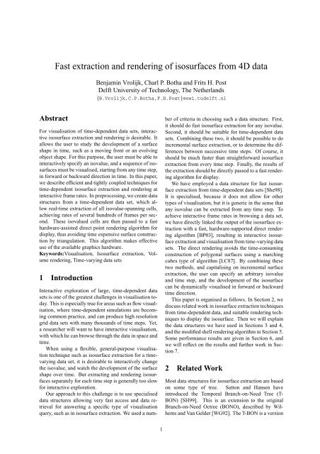
Figure 5 shows a single timestep of a sample dataset
rendered with the ShellSplatter and the fast point-based
renderer. The ShellSplatted rendering on the left shows
the typical fuzziness often associated with splattingbased
rendering methods whilst the fast point-based
rendering on the right appears slightly jagged due to
the use of flat-shaded quads.
6 Results
We have used two data sets for testing the performance
of the THITree and the renderer. The first is a
61×50×60 synthetic data set of a moving spherical isosurface,
with a maximum of 55 time steps (“sphere”).
The second data set is obtained from a fluid dynamics
simulation, and contains turbulent vortex structures 1 .
The size of this data set is 64 3 × 64 time steps (“vorticity”).
The extraction and rendering performance have been
measured on a 2.4 GHz Pentium 4 with 1 GB of memory
and a 128 MB GeForce 4 Ti4600 graphics card.
1 Data courtesy D. Silver and X. Wang of Rutgers University.
7
6.1 THITree size
The memory size of the Temporal Hierarchical Index
Tree for the 55 time steps of the sphere data set is about
75 Megabytes. The vorticity data set results in a tree
size of about 640 Megabytes. This huge difference has
to do with the variability of the data and can be illustrated
by examining the number of cells in each of the
nodes of the tree.
There are two parameters that influence the size of
the data structure, and thereby of course, also performance
and accuracy.
First, the size of the Span Space can be changed, that
is, the number of rows or columns in the Span Space.
This affects the number of cells in each row, the number
of Interval Trees in the Span Space (one for each row),
and the number of cells that has to be stored in each
Interval Tree.
However, the total number of cells in the Span Space
is not affected, therefore, the memory size of the Span
Space will hardly change. Only the vector representing
the Span Space boundaries is affected by this parameter,
but this vector is stored only once for the entire
THITree. But if the Span Space contains fewer grid elements,
meaning that the grid elements are larger, then
cells will sooner be considered constant for a longer
time span, and therefore these cells will be stored higher
up in the THITree, thus reducing the overall size of the
data structure. The downside is that more false positives
will be found. Accuracy is traded off for memory
size.
The same applies to the MaxVariation parameter,
which indicates how many grid elements cells may
span, and still be considered constant. Thus, without
changing the size of each Span Space, we can control
the level at which the cells will be stored in the
THITree. This way we are able to reduce the total memory
size of the tree, but at the cost of increasing the
number of false positives that will be found.
In Tables 1 and 2 a few performance characteristics
of the Temporal Hierarchical Index Tree are shown. We
have used the sphere data set (61 × 50 × 60) for determining
the influence of the two parameters discussed
above. We used sequences of 25 and 55 time steps, and
created THITrees with 3 variants of each of the two parameters:
for the Span Space size, we used values of
32, 64 and 128, and for the MaxVariation we used 1, 2
and 3 grid elements.
Cells in our data structure are represented by a cell
id, a minimum and maximum value, and a gradient. We
compared the size of the THITree to the raw data size,
meaning simply the number of time steps × the number
of cells × the memory size of one cell.
The percentage of false positives indicates how
many cells are returned that do not contain the isovalue
in the current time step.

Figure 5: Example renderings of a single time step. On the left the high quality ShellSplatting is shown, on the
right the faster simple point-based renderer output is shown.
Data set size: 61 × 50 × 60
MaxVariation in Span Space: 2 cells
SpanSpaceSize 32 64 128
# timesteps 25 55 25 55 25 55
THITree size (MB) 26.0 48.9 38.7 75.5 59.3 111.9
% of raw data 25.0% 21.4% 37.2% 33.0% 57.0% 48.9%
% false positives 5.3% 2.1% 1.3% 0.5% 0.3% 0.1%
Search (ms) 2.12 2.45 2.14 2.86 1.97 2.50
SearchIncr (ms) 0.46 0.65 0.74 0.88 0.89 1.00
Speed up 4.64 3.75 2.90 3.26 2.21 2.50
Table 1: Time and space performance of the THITree for three values of SpanSpaceSize.
Data set size: 61 × 50 × 60
SpanSpaceSize: 64
MaxVariation 1 cell 2 cells 3 cells
# timesteps 25 55 25 55 25 55
THITree size (MB) 121.0 246.4 38.7 75.5 27.4 52.2
% of raw data 116.2% 107.6% 37.2% 33.0% 26.3% 22.8%
% false positives 0.09% 0.08% 1.3% 0.5% 3.9% 1.4%
Search (ms) 2.07 2.32 2.14 2.86 2.36 2.93
SearchIncr (ms) 0.93 0.83 0.74 0.88 0.59 0.88
Speed up 2.23 2.79 2.90 3.26 4.00 3.34
Table 2: Time and space performance of the THITree for three values of MaxVariation.
8

Rendering mode Sphere Vorticity
High quality 50.30 46.29
Fast 250.85 284.42
Table 3: Average rendering frame rates (in FPS) for the
two data sets, both in high quality and in fast rendering
mode.
6.2 Surface cell extraction
The THITree data structure provides a very quick way
to search for isosurface cells. In our sphere data set
the time for extraction of the isosurface cells for a single
time step takes on average approximately 2.25 milliseconds.
When we use the incremental search algorithm
we can achieve even higher rates: incrementally
searching the isosurface cells in 55 consecutive time
steps costs about 43 milliseconds. This corresponds to
more than 1250 frames per second. In the vorticity data
set the average rate of extraction for the 64 time steps is
more than 4000 frames per second.
Referring to Tables 1 and 2, the row “Search (ms)”
displays the average extraction time (in milliseconds)
of the isosurface cells from a single time step. The next
row shows the same, but with the use of our incremental
search routine 2 . The last row shows the speed-up of the
incremental search, compared to the normal search.
6.3 Rendering performance
We have tested the two renderers, both the high quality
ShellSplatter and the lower quality fast point-based
renderer, with the two data sets. The average frame
rates for the total pipeline of extraction and rendering
are shown in Table 3.
Compared to the extraction times, the rendering is
the bottleneck. The numbers in this Table are rates for
combined extraction and rendering, but 99% of the time
is used in the rendering step. For the rendering, the
number of isosurface cells is the most important factor.
The average number of isosurface cells extracted from
the sphere data set is 3760, without much variation over
time. For the vorticity data set, the number of isosurface
cells ranges from about 1500 to 8700, with an average
of 3940 cells per time step.
7 Conclusions and future work
We have described techniques for fast isourface extraction
and direct rendering from time-varying data
sets. In a preprocessing step, data structures are generated
that allow us to retrieve the isovalue-spanning
cells at any time step and for any isovalue with high
2 These timings were measured on a dual AMD Athlon MP 1.2
GHz machine.
9
frame rates. Incremental searching uses temporal coherence
to further speed up the extraction process. The
extracted cells are rendered directly with a fast pointbased
rendering technique, displaying a shaded quadrangle
at each pixel at high frame rates. No visibility
ordering is needed in this case, so the overall speed is
not reduced by an intermediate data conversion step.
A high quality rendering technique based on Shell-
Splatting does require visibility ordering, but can still
achieve high frame rates for a 64 3 data set. In an interactive
environment, the fast rendering can be used during
interaction, while the high quality technique can be
automatically invoked when the input queue is empty.
We will integrate this in our VR data exploration system.
In this work we have concentrated on fast access and
the integration of rendering, and we did not try to solve
the problem of the size of the search data structures.
However, this size is definitely too large and should be
reduced considerably to make the technique truly scalable
to very large data sets. There is still room for improvement
in our current implementation of the tree, for
example by storing the two vectors AL and DR more
efficiently. Another possible improvement would be
the use of a separate Span Space subdivision at each
of the THITree nodes, instead of using the same subdivision
throughout the tree. It may also be worth looking
into leaving out the Span Space entirely and just using
one large Interval Tree at each of the THITree nodes.
Further improvements are possible by using compression
techniques, as recently proposed by Bordoloi and
Shen [BS03].
There are two possible sources of error in the display
of the isosurfaces that must be investigated further. Although
this did not show up in the test images, the rendering
of false positive cells may cause artifacts. Also,
the surface normals are stored only once over a time interval
that is considered “more or less constant”. This
also did not have any noticeable effect in the images,
but we will analyse the extent of the errors caused.
Acknowledgements
This project was partly supported by the Netherlands
Organisation for Scientific Research (NWO) on the
NWO-EW Computational Science Project “Direct Numerical
Simulation of Oil/Water Mixtures Using Front
Capturing Techniques”.
This research was partly supported by the DIPEX
(Development of Improved endo-Prostheses for the upper
EXtremities) program of the Delft Interfaculty Research
Center on Medical Engineering (DIOC-9).

References
[BP03] Charl P. Botha and Frits H. Post.
ShellSplatting: Interactive rendering of
anisotropic volumes. In G.-P. Bonneau,
S. Hahmann, and C. D. Hansen, editors,
Data Visualization 2003 (Proceedings
of Joint Eurographics - IEEE TCVG
Symposium on Visualization). ACM SIG-
GRAPH, 2003.
[BS03] Udeepta D. Bordoloi and Han-Wei Shen.
Space efficient fast isosurface extraction
for large datasets. In Proc. IEEE Visualization
’03, pages 201–208, 2003.
[CMM + 97] P. Cignoni, P. Marino, C. Montani,
E. Puppo, and R. Scopigno. Speeding up
isosurface extraction using interval trees.
IEEE TVCG, 3(2):158–170, April–June
1997.
[Ede80] H. Edelsbrunner. Dynamic data structures
for orthogonal intersection queries. Technical
Report F59, Inst. Informationsverarb.,
Tech. Univ. Graz, Graz, Austria,
1980.
[IEE99] 1999.
[KM01] Steven Kilthau and Torsten Möller. Splatting
optimizations. Technical report, Simon
Fraser University, 2001.
[LC87] William E. Lorensen and Harvey E. Cline.
Marching cubes: A high resolution 3D
surface construction algorithm. In Proc.
SIGGRAPH, pages 163–169, 1987.
[LSJ96] Y. Livnat, Han-Wei Shen, and C. R. Johnson.
A near optimal isosurface extraction
algorithm using the span space. IEEE
TVCG, 2(1):73–84, March 1996.
[RL00] Szymon Rusinkiewicz and Marc Levoy.
Qsplat: A multiresolution point rendering
system for large meshes. In Kurt Akeley,
editor, Proc. SIGGRAPH, pages 343–352,
2000.
[RPZ02] Liu Ren, Hanspeter Pfister, and Matthias
Zwicker. Object space EWA surface splatting:
A hardware accelerated approach to
high quality point rendering. Computer
Graphics Forum, 21(3):461–470, 2002.
[SCM99] Han-Wei Shen, L.-J. Chiang, and K.-L.
Ma. A fast volume rendering algorithm
for time-varying fields using a time-space
partitioning (tsp) tree. In Proc. IEEE
Visualization ’99 [IEE99], pages 371–
377,545.
10
[SH99] P. Sutton and C. D. Hansen. Isosurface
extraction in time-varying fields using a
temporal branch-on-need tree (T-BON).
In Proc. IEEE Visualization ’99 [IEE99],
pages 147–153,520.
[She98] Han-Wei Shen. Isosurface extraction in
time-varying fields using a temporal hierarchical
index tree. In Proc. IEEE Visualization
’98, pages 159–166, 1998.
[SHLJ96] Han-Wei Shen, C. D. Hansen, Y. Livnat,
and C. R. Johnson. Isosurfacing in span
space with utmost efficiency (issue). In
Proc. IEEE Visualization ’96, pages 287–
294, 1996.
[SMC01a] B. Stenger, P. R. S. Mendonça, and
R. Cipolla. Model based 3D tracking of
an articulated hand. In Proc. Conf. Computer
Vision and Pattern Recognition, volume
II, pages 310–315, Kauai, USA, dec
2001.
[SMC01b] B. Stenger, P. R. S. Mendonça, and
R. Cipolla. Model-based hand tracking using
an unscented kalman filter. In Proc.
British Machine Vision Conference, volume
I, pages 63–72, Manchester, UK, sep
2001.
[UO93] Jayaram K. Udupa and Dewey Odhner.
Shell rendering. IEEE CG&A, 13(6):58–
67, November 1993.
[Wes89] Lee Westover. Interactive volume rendering.
In Proceedings of the Chapel Hill
workshop on Volume Visualization, pages
9–16, Chapel Hill, NC, USA, 1989. ACM
Press.
[WG92] Jane Wilhelms and Allen Van Gelder.
Octrees for faster isosurface generation.
ACM Transactions on Graphics,
11(3):201–227, July 1992.