Master Thesis - Computer Graphics and Visualization - TU Delft

Unbiased Rendering 2.4 Path Tracing
Y 0
Y 1
Y 2
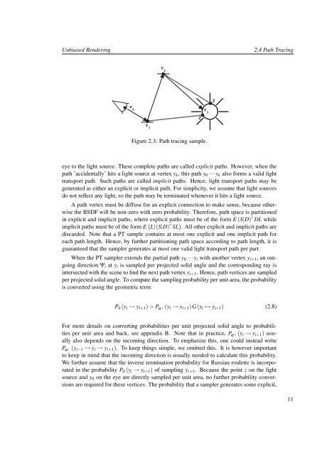
Figure 2.3: Path tracing sample.
eye to the light source. These complete paths are called explicit paths. However, when the
path ’accidentally’ hits a light source at vertex yk, this path y0 ···yk also forms a valid light
transport path. Such paths are called implicit paths. Hence, light transport paths may be
generated as either an explicit or implicit path. For simplicity, we assume that light sources
do not reflect any light, so the path may be terminated whenever it hits a light source.
A path vertex must be diffuse for an explicit connection to make sense, because otherwise
the BSDF will be non-zero with zero probability. Therefore, path space is partitioned
in explicit and implicit paths, where explicit paths must be of the form E (S|D) ∗ DL while
implicit paths must be of the form E L|(S|D) ∗ SL . All other explicit and implicit paths are
discarded. Note that a PT sample contains at most one explicit and one implicit path for
each path length. Hence, by further partitioning path space according to path length, it is
guaranteed that the sampler generates at most one valid light transport path per part.
When the PT sampler extends the partial path y0 ···yi with another vertex yi+1, an outgoing
direction Ψi at yi is sampled per projected solid angle and the corresponding ray is
intersected with the scene to find the next path vertex yi+1. Hence, path vertices are sampled
per projected solid angle. To compute the sampling probability per unit area, the probability
is converted using the geometric term:
PA (yi → yi+1) = P σ ⊥ (yi → yi+1)G(yi ↔ yi+1) (2.8)
For more details on converting probabilities per unit projected solid angle to probabilities
per unit area and back, see appendix B. Note that in practice, P σ ⊥ (yi → yi+1) usually
also depends on the incoming direction. To emphasize this, one could instead write
P σ ⊥ (yi−1 → yi → yi+1). To keep things simple, we omitted this. It is however important
to keep in mind that the incoming direction is usually needed to calculate this probability.
We further assume that the inverse termination probability for Russian roulette is incorporated
in the probability PA (yi → yi+1) of sampling yi+1. Because the point z on the light
source and y0 on the eye are directly sampled per unit area, no further probability conversions
are required for these vertices. The probability that a sampler generates some explicit,
Z
Y 3
Z
11