On the Optimal Taxation of Capital Income
On the Optimal Taxation of Capital Income
On the Optimal Taxation of Capital Income

You also want an ePaper? Increase the reach of your titles
YUMPU automatically turns print PDFs into web optimized ePapers that Google loves.
114 JONES, MANUELLI, AND ROSSI<br />
<strong>of</strong> which is able to supply one unit <strong>of</strong> leisure to <strong>the</strong> market each period.<br />
Our specification <strong>of</strong> technology is similar to <strong>the</strong> nested CES model<br />
estimated by Kwag and McMahon [18]. They consider a setting in which<br />
<strong>the</strong> inner function is a CES between skilled labor and physical capital; this<br />
aggregate, in turn, is combined using ano<strong>the</strong>r CES with unskilled capital.<br />
They estimate that <strong>the</strong> elasticity <strong>of</strong> substitution between physical capital<br />
and skilled labor is very low (i.e., 0.013), while that between <strong>the</strong> combined<br />
total capital and low skilled labor is in <strong>the</strong> range <strong>of</strong> 0.482 to 0.769. Guided<br />
by this we assumed that <strong>the</strong> elasticity <strong>of</strong> substitution between n 2 and <strong>the</strong><br />
composite between n 1 and k is one to simplify <strong>the</strong> analysis, and we set<br />
\=5.0 (which corresponds to an elasticity <strong>of</strong> 0.16 between capital and<br />
skilled labor). This is <strong>the</strong> rationale behind our interpretation <strong>of</strong> n 1 as<br />
skilled labor and n 2 as unskilled labor. We chose _=2, =0.9, # 1=&0.2,<br />
and # 2=&0.8 as a base case and chose g so that <strong>the</strong> budget would exactly<br />
balance with a flat income tax rate <strong>of</strong> 200 on all sources <strong>of</strong> income.<br />
We calculated <strong>the</strong> solution to <strong>the</strong> planner's problem (see Jones, Manuelli<br />
and Rossi [13] for a detailed discussion <strong>of</strong> <strong>the</strong> methods) both from a wide<br />
range <strong>of</strong> initial capital stocks and with and without imposing bounds (<strong>of</strong><br />
1000) on <strong>the</strong> capital income tax rate along <strong>the</strong> path to <strong>the</strong> steady state.<br />
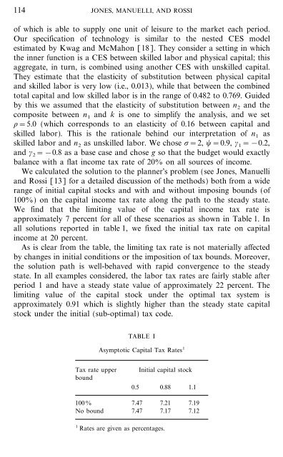
We find that <strong>the</strong> limiting value <strong>of</strong> <strong>the</strong> capital income tax rate is<br />
approximately 7 percent for all <strong>of</strong> <strong>the</strong>se scenarios as shown in Table 1. In<br />
all solutions reported in table 1, we fixed <strong>the</strong> initial tax rate on capital<br />
income at 20 percent.<br />
As is clear from <strong>the</strong> table, <strong>the</strong> limiting tax rate is not materially affected<br />
by changes in initial conditions or <strong>the</strong> imposition <strong>of</strong> tax bounds. Moreover,<br />
<strong>the</strong> solution path is well-behaved with rapid convergence to <strong>the</strong> steady<br />
state. In all examples considered, <strong>the</strong> labor tax rates are fairly stable after<br />
period 1 and have a steady state value <strong>of</strong> approximately 22 percent. The<br />
limiting value <strong>of</strong> <strong>the</strong> capital stock under <strong>the</strong> optimal tax system is<br />
approximately 0.91 which is slightly higher than <strong>the</strong> steady state capital<br />
stock under <strong>the</strong> initial (sub-optimal) tax code.<br />
Tax rate upper<br />
bound<br />
TABLE I<br />
Asymptotic <strong>Capital</strong> Tax Rates 1<br />
Initial capital stock<br />
0.5 0.88 1.1<br />
1000 7.47 7.21 7.19<br />
No bound 7.47 7.17 7.12<br />
1 Rates are given as percentages.