Fisher Separation Theorem & Consumer Optimization 1. TWO ...

FINANCIAL ECONOMICS Clemson Economics 

Fisher Separation Theorem & Consumer Optimization 

1. TWO-PERIOD CONSUMPTION AND INVESTMENT IN ABSENCE OF RISK 

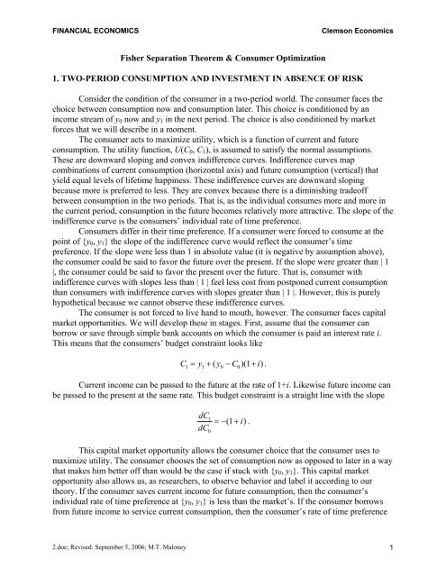
Consider the condition of the consumer in a two-period world. The consumer faces the 

choice between consumption now and consumption later. This choice is conditioned by an 

income stream of y0 now and y1 in the next period. The choice is also conditioned by market 

forces that we will describe in a moment. 

The consumer acts to maximize utility, which is a function of current and future 

consumption. The utility function, U(C0, C1), is assumed to satisfy the normal assumptions. 

These are downward sloping and convex indifference curves. Indifference curves map 

combinations of current consumption (horizontal axis) and future consumption (vertical) that 

yield equal levels of lifetime happiness. These indifference curves are downward sloping 

because more is preferred to less. They are convex because there is a diminishing tradeoff 

between consumption in the two periods. That is, as the individual consumes more and more in 

the current period, consumption in the future becomes relatively more attractive. The slope of the 

indifference curve is the consumers’ individual rate of time preference. 

Consumers differ in their time preference. If a consumer were forced to consume at the 

point of {y0, y1} the slope of the indifference curve would reflect the consumer’s time 

preference. If the slope were less than 1 in absolute value (it is negative by assumption above), 

the consumer could be said to favor the future over the present. If the slope were greater than | 1 

|, the consumer could be said to favor the present over the future. That is, consumer with 

indifference curves with slopes less than | 1 | feel less cost from postponed current consumption 

than consumers with indifference curves with slopes greater than | 1 |. However, this is purely 

hypothetical because we cannot observe these indifference curves. 

The consumer is not forced to live hand to mouth, however. The consumer faces capital 

market opportunities. We will develop these in stages. First, assume that the consumer can 

borrow or save through simple bank accounts on which the consumer is paid an interest rate i. 

This means that the consumers’ budget constraint looks like 

C = y + ( y − C )( + i). 

1 1 0 0 1 

Current income can be passed to the future at the rate of 1+i. Likewise future income can 

be passed to the present at the same rate. This budget constraint is a straight line with the slope 

dC 

dC 

1 

0 

=− ( 1+ 

i). 

This capital market opportunity allows the consumer choice that the consumer uses to 

maximize utility. The consumer chooses the set of consumption now as opposed to later in a way 

that makes him better off than would be the case if stuck with {y0, y1}. This capital market 

opportunity also allows us, as researchers, to observe behavior and label it according to our 

theory. If the consumer saves current income for future consumption, then the consumer’s 

individual rate of time preference at {y0, y1} is less than the market’s. If the consumer borrows 

from future income to service current consumption, then the consumer’s rate of time preference 

2.doc; Revised: September 5, 2006; M.T. Maloney 1


at {y0, y1} is greater than the market’s. In the absence of any productivity of investment, the 

market rate of interest would be determined by the relative number of people willing to borrow 

or lend. 1 Notice that as the budget line pivots on the point {y0, y1} as the interest rate changes 

any consumer can shift from being a lender to becoming a borrower if the interest rate falls 

sufficiently. This is the demand for borrowing/supply of savings function. Still, individuals vary 

in their relative demand/supply. 

Next, assume that the consumer has the opportunity to invest his savings (if he chooses to 

save) in productive capital projects. Let there be an investment productivity function that maps 

savings into future income. This project curve starts at the point {y0, y1}; initially its slope is 

steeper than the bank borrowing line (capital market line), but the slope diminishes as more is 

invested. The slope of this investment productivity function represents the marginal return on 

individual investment opportunities. The individual chooses the level of investment that 

maximizing utility. In the absence of access to the capital market, the consumer chooses to invest 

up to the point where the slope of the investment productivity frontier is equal to the slope of the 

indifference curve that is tangent to it. This is the highest level of utility achievable by the 

consumer. It also has the characteristic that the consumer’s individual rate of time preference is 

equal to the marginal return on investment; call this, r. 

Finally, if the consumer has both the availability of productive investment projects and 

access to the capital market, the individual can expand utility even further. In this world the 

consumer invests along the capital project frontier up to the point where the marginal rate of 

return implied by the slope of this frontier is equal to the interest rate. That is, investment occurs 

until r is equal to i. The consumer then either borrows or lends beyond this tangency to the point 

where the highest indifference curve is tangent to this “expanded” capital market line. The 

efficient capital project level has a payoff of P1-y1 from the investment y0-P0. 

2. OPTIMAL INVESTMENT 

This result is called the Fisher Separation Theorem. It says that in the presence of perfect 

capital markets, the consumer’s investment and consumption decisions are independent. All 

consumers invest along their capital project frontiers to the point where r = i, and then borrow or 

save to satisfy their own personal rate of time preference. The Theorem has a number of 

important implications: 

1. All investment opportunities are exploited. 

2. All investment opportunities are priced the same, that is, priced by the same condition, r=i. 

3. Efficient management of investment projects is achieved by maximizing the present value of 

the investment. That is, max P1 occurs where dP1 / dP0 = (1+i). (Note that the minus sign goes 

away because P0 is measured backwards on the horizontal axis.) Or in present value terms, 

dP 

0 

dP1 

= . 

1+ 

i 

1 This number is generally determined by life cycle forces in context of multi-period models⎯things like lifetime 

wage profiles. 



This last point leads us to the conclusion that firms, which are the economic agents that 

manage production and investment, should act to maximize present value. 

3. WEALTH, RISK, & UTILITY 

Next we begin to develop the Capital Asset Pricing Model, or CAPM. CAPM attempts to 

explain the way that assets like stocks and bonds are priced. It does this without resorting to 

idiosyncratic characteristics. 

Science is empirical and the best science is empirical and elegant. I like to think of the 

best, most elegant scientific theories as magic tricks. It is like pulling a rabbit out of a hat. 

Demand Theory is like this. Demand theory starts with the absolutely unobservable notion of a 

utility function and from that, derives completely empirical predictions. Similarly, CAPM starts 

with what seems to be a “tired” definition of risk aversion and then is able to explain nearly all 

of the cross-sectional variation in the prices of securities. 

We start with the theory of the utility of wealth when the level of wealth is uncertain. 

Before we begin, there are a couple of statistical properties that are useful to understand. 

First, we define the notion of expected value. E( x) = ∑ px , that is, the expected value 

of the random variable x is the probability times the value of x summed over all possible values 

that x can take. A probability function defines all of these and sums the associated probabilities 

to 1. For continuous distributions, the density function replaces pi. For the normal this is 

1 

nx ( )= e 

σ 2π 

F 

2 

1 x−µ 

I − HG KJ 2 σ 

The continuous density is integrated rather than summed over its range. The integral of 

the density is 1 and the expected value of x is µ. 

z+∞ 

−∞ 

nx ( ; µσ , ) dx= 

1 

z z 

2 

1F 

x−µ 

I +∞ 

+∞ 1 − 

σ 

Ex ( ) xnx ( ; µσ , ) dx x e 

HG KJ 2 

= ⋅ = ⋅ dx= 

µ 

−∞ 

−∞ σ 2π 

From the definition of expected value we can derive the result that the expected value of 

x plus a constant a is just a plus the expected value of x. Similarly, the expected value of x times 

a constant is the constant times the expected value of x. 

2 

The second definition is that of the variance. Var( x) = E[( xi − E( x)) 

] . Applying the 

2 

definition of the expected value, we have Var( x)= 

p ( x − E( x)) 

. From this definition, rules 

of association also follow. The variance of a random variable x plus a constant a is equal to the 

variance of x alone. The constant falls out. Next, the variance of x times a constant is equal to the 

constant squared times the variance of x. 

2.doc; Revised: September 5, 2006; M.T. Maloney 3 

∑ 

i 

i 

i 

i i


Axioms of choice 

• Comparability (Completeness) 

• Transitivity 

• Strong Independence 

A gamble involving x and z will yield the same utility as an identical gamble involving y 

and z if consumer is indifferent between x and y. 

• Measurability 

If y is preferred to x and z is preferred to y, there exists a gamble involving x and z to 

which the consumer is indifferent compared to y. 

• Ranking 

If both y and u lie between x and z, the gamble that equates {x, z} to y can be compared to 

the gamble that equates {x, z} to u. If the probability associated with x in the y-equivalent 

gamble is greater than the probability associated with x in the u-equivalent gamble, then 

u is preferred to y. 

Utility of Risky Outcomes 

Define risky events in terms of a gamble. That is, let’s say that a consumer will receive x 

dollars with probability α and z with probability (1-α). The expected value of this is some 

number, call it y. In a gamble, the consumer does not get the expected value. The consumer gets 

either x or z. That is the problem. The question is, Does the consumer like the gambling nature of 

the problem? That is, would the consumer be happier with y or happier with the gamble, which 

will yield either x or z. 

To answer this, let’s define the consumer’s utility in the event of the gamble. The utility 

of x is U(x) and the utility of z is U(z). The consumer’s expected utility from the gamble is, then, 

αU(x)+(1-α)U(z). This is called the expected utility of uncertain wealth, or E(U(W)). 

We can compare the expected utility of uncertain wealth to the utility of certain wealth 

that has the same expected value as the gamble. Call this the utility of expected wealth, or 

U(E(W)). In our example, the utility of expected wealth is the utility level associated with the 

dollar value y because that is the expected value of a gamble. So, U(E(W)) = U(y). This is not the 

utility of the gamble. The utility of expected wealth is the utility of the money- certain value of 

the expected value of the risky outcome. On the other hand, the expected utility of uncertain 

wealth is the utility of the gamble itself. 

Expected utility is the utility of the wealth outcome in each possible event times the 

probability of that event, 

1. EU ( ) = ∑ U( x) px ( ) 

or in continuous terms it is the utility of wealth at each level of x times the continuous density of 

x, integrated over all possible values: 

=z 

2. EU ( ) U( x) f( xdx ) 



If the utility of the money-certain expected value of the risky outcome is greater than the 

expected utility of the risky outcome, then the consumer is labeled risk averse. The picture tells 

the story. 

From the picture, we can see how much in money terms the consumer will pay to avoid 

risk, for risk averse consumers. For risk-loving consumers we can see how much the consumer 

will pay to gamble. Friedman and Savage drew a little picture to try to explain how a consumer 

could be a gambler and an insurer all at the same time. 2 Cute. Their theory has a few holes, but 

generally it is a reasonable way to think about this problem. We are not so much interested in 

refining our understanding of utility theory, but rather, we want to put the definition of risk 

aversion to work with wealth maximization. 

Mean-Variance Paradigm 

To do this, let’s look at the risky world in terms of the appreciation of assets. Let the 

appreciation of wealth of wealth be defined as: 3 

W −W 

R = 

W 

1 0 

The expected value of the appreciation of wealth is: 

EW ( 1) 

E( R) 

= −1 

W 

which, based on our discussion at the beginning of this lecture, is distributed with a variance: 

σ 

2 

R 

0 

0 

σ 

= 

W 

Utility can be defined in terms of the appreciation in the value of wealth, which is defined by its 

expected value and its standard deviation: 

2 

w 

2 

0 

U = U( W , R( E( R), 

σ ) ) 

0 

In this way the expected value of utility can be defined. Using the continuous distribution 

formula, the expected value of utility is the integral of utility over each value of the appreciation 

of wealth times the density at that value: 

= z−∞ 0 2 

+∞ 

3. EU ( ) UW ( , R) f( RER ; ( ), σ ^ ) dR 

2 

Friedman and Savage, “Utility Analysis of Choices Involving Risk,” JPE, 1948, in AEA Readings in Price 

Theory. 

3 

The book is a bit idiosyncratic in this regard, suggesting that the wealth of an individual is tied up in one asset. 

This is not the right way to think about the problem. Assume that wealth is held in a diversified portfolio of assets. 



Assume that the distribution of the return on wealth is normal. That is, let f(.)=n(.). Then 

we can use the normal variant: 

R− E( R) 

Z = 

σ 

Rewriting in terms of R gives: 

R = E( R) + σ Z 

Substituting this into the expected utility function gives: 

z = 0 + 

4. EU ( ) UW ( , E( R) σ Z) nZ ( ; 01 , ) dZ 

Note that (4) is just the same expression as (1) and (2) above. It is the expected value of 

utility, which is given by multiplying the utility value at each uncertain wealth level times the 

associated probability and summing these products. 

Next, take the total differential of (4) and set this equal to zero: 

z = ′ 0 + + 

b g 

dE( U ) U ( W , E( R) σZ) dE( R) Zdσ n( Z; 01 , ) dZ = 0 

This differential can be factored, 

z z 

dE( R) U ′ ( W0, E( R) + σZ) n( Z; 01 , ) dZ + dσ U ′ ( W0, E( R) + σZ) 

⋅Z⋅ n( Z; 01 , ) dZ = 0 

and solved for the derivative of the expected return w.r.t. the standard deviation: 

5. 

z z 

dE( R) 

U′ ( W0, E( R) + σZ) 

⋅Z⋅n( Z; 01 , ) dZ 

=− 

> 0 

dσ 

U′ ( W , E( R) + σZ) 

n( Z; 01 , ) dZ 

0 

What we have here is the slope of the indifference curve between risk and return. It is 

positively sloped. The denominator is positive. The denominator is just marginal utility, which is 

positive, times the normal density and integrated over all values. This is the expected value of 

marginal utility. Not a particularly empirical value, but clearly positive by definition. 

The numerator of (5) is negative. This is so because it is marginal utility times Z times 

the normal density and then summed over all values. The unit normal variate, Z, takes values 

from minus to plus infinity and is centered on zero. This means that values of marginal utility 

that are below the mean wealth are weighted by negative Z values and values of marginal utility 

above the mean wealth are weighted by positive Z values. 

This is precisely the point that our definition of risk aversion comes into play. Risk 

aversion means that lower wealth has a higher marginal utility than higher wealth. See the wealth 

and utility picture. Multiplying high marginal utility in the numerator of (5) Z weighted marginal 

utility is negative. Hence, the negative numerator cancels the negative sign in front and (5) is 

positive. 



This derivation shows that the definition of risk aversion developed by drawing the 

distinction between expected utility of uncertain wealth and the utility of the certain money 

equivalent of the expected value of wealth can be translated into consumer indifference curves 

defined in terms of the expected return on wealth and the standard deviation (or risk) of that 

return. Indifference curves that measure the utility-constant tradeoff between expected return and 

risk are positively sloped. (They are also convex, which can be shown by taking the second 

derivative, that is, differentiating (5) w.r.t. s. However, we will eschew that exercise in the 

interest of avoiding sleeping sickness.) 

As noted above, some commentators claim that the mean-variance paradigm is flawed 

and limited because it is founded on the assumption that the return on wealth is normally 

distributed. Truly, in the derivation that is shown above, the normal distribution is fully 

exploited. It is not likely that any of us could take the total differential of (3). It is only by 

converting (3) into (4) using the assumption of normality that the problem becomes tractable. 

However, there is nothing wrong with simplifying a model by making assumptions. That 

is the scientific method. To say that the mean-variance paradigm is incomplete because we have 

assumed that the distribution of the return on wealth is normal, is like saying that the theory of 

gravity is incomplete. No doubt, it is. Works pretty good, though. 

Even so, we still stand on higher ground. The distribution of the return on wealth is most 

appropriately modeled as normal based on the Central Limit Theorem. If wealth is held in a welldiversified 

portfolio, the return is the average of the returns to many assets. As such this portfolio 

return is a sample mean. Sample means are normally distributed. 4 

At this point in the development of the Capital Asset Pricing Model, which I think of as 

akin to pulling a rabbit out of a hat, all we have done is show that the hat is empty. By this, I 

mean that we have set the stage. We have defined the basis for utility maximization by 

identifying a utility function and showing what it means in the dimension that we can observe 

real world assets. However, utility itself is a non-observable thing. Hence, to get stock prices out 

of this model, we are going to have to do some tricky work. 

Addendum on Preference Theory 5 

Lottery Construct 

Define a simple lottery as L= ( p ,..., p ) where p = 1. 

1 

N 

Compound Lottery: A simple lottery can be the combination of other lotteries called compound 

1 

K 

lotteries: p =α p + ... +α p 

i 1 i K i 

Axioms of Preference: 

0 1 

Continuous: Consider L L L . There exists an α such that: 

2 

0 2 1 

α L + (1 −α) L ∼ L 

4 

If a person’s wealth were tied up in a single event (like, for instance, one’s graduate education) then the 

distribution would arguably be binomial. 

5 

Mostly from Ch. 6, Mas-Colell, Whinston, and Green, Microeconomic Theory, Oxford Press. 


∑ 

N 

i


0 1 

Independence: Consider L L . Adding an alternative does not affect the ranking: 

0 2 1 

2 

α L + (1 −α) L α L + ( 1 −α) 

L 

This is quite different from consumer theory under uncertainty and leads to some paradoxes. 

Von Neumann-Morgenstern expected utility function: 

If there exists a set {u1,...,uN} such that for every simple lottery L= ( p1,..., pN) 

we have a utility 

function U L , then that function is of the vN-M expected utility form. 6 

= u p + + u p 

( ) 1 1 ... N N 

With the vN-M expected utility form, the utility of a lottery can be thought of as the expected 

value of the utilities, ui, of the N outcomes. 

Expected utility form is linear: U( ∑α kL k) = ∑αkU( 

Lk) 

vN-M expected utility functions are transformable by linear operators: 

U ( L) =β U( L) 

+γ 

U α L =βU α L +γ = α β U L +γ = αU 

L) 

( ∑ ) ( ∑ ) ∑ [ ( ) ] ∑ ( 

u 

These are cardinal utility functions. The difference in the level of utility matters. 

u − u > u − u => .5 u + .5 u > .5 u 

0 1 

+ .5 => L = (.5,0,0,.5) L = (0,.5,.5,0) 

1 2 3 

4 1 4 2 3 

Allais’ Paradox: 

1 st prize: $25 mil.; 2 nd prize: $5 mil; 3 rd prize: 0. 

4 lotteries: 

0 

L = (0,1,0) 

1 

L = (.1,.89,.01) 

1 

1 

L 

L 

0 

2 

1 

2 

= (0,.11,.89) 

= (.1,0,.9) 

0 

Assume that L L ; how do the last two compare. Note that 

1 0 

1 1 

1 0 

2 2 

1 

1 

1 

L = L + (.1, −.11,.01) 

L = L + (.1, −.11,.01) 

Therefore it should be true that: 

0 1 

L L 

2 2 

Most people will probably not rank this way. What does it mean? 

6 Note that the lottery setup simply allows us to consider multiple outcome. The actual utility function that maps 

these outcomes in a von Neumann-Morgenstern way can be as simple as U=ln(W) if we are only concerned with 

monetary bundles. 



Risk Aversion: 

The utility of certain wealth is greater than the expectation of the utility of the wealth outcomes 

that are equivalent to that certain wealth. 

∫ ∫ 

( ) 

uwdFw ( ) ( ) 

(Draw concave function in utility and wealth space.) Consider W ± ε. Let c(ε) be the certain 

wealth that yields the same utility as the expected value of the uncertain outcomes around W. 

Let π(ε) be the adjustment in probability that makes the consumer indifferent to certain wealth of 

W and the uncertain outcome, i.e., 

[.5 +π ]( W +ε ) + [.5 −π]( W −ε ) 

(interpret via picture) 

Insurance: 

Initial wealth: W; probability of loss D: ρ. 

Outcome without insurance: ( 1 −ρ ) W +ρ( W −D) 

Insurance: q is cost of insurance per $1 of coverage; A is the amount of coverage. 

Outcome with insurance: (1 −ρ)( W − Aq) +ρ( W − Aq− D+ A) 

Consumer maximizes: 

max Z = (1 −ρ) uW ( − Aq) +ρuW ( − Aq− D+ A) 

{ A} FOC: 

−q(1 −ρ ) u'(no loss) +ρ(1 − q) u'(loss) 

= 0 

Let insurance be competitive and have no admin or agency costs: q = ρ. Thus, 

u'(no loss) = u'(loss) 

=> => A * ( W − Aq) = ( W − Aq− D+ A) 

= D 

If the consumer can insure at actuarially fair rates, the risk averse consumer will fully insure. 7 

Choice with Risky Assets: 

Safe Asset: zero return; no risk. $1 maintains its value with certainty. 

∫ 

Risky Asset: return of r such that (1 + rdFr ) ( ) > 1; 

that is, $1 in the risky asset will on average 

be worth more than $1 at the resolution of uncertainty. 

Initial wealth, W; A is the amount of W in the risky asset; B is the amount in the safe asset. 

Consumer’s problem: 

∫ 

max { AB , } uA ( ⋅ (1 + r) + BdFr ) ( ) s.t. A+ B= W 

or 

7 SSOC show that it is only the risk averse consumer that does this: u''


∫ 

∫ 

max { A} uW ( + A⋅r]) dF( r) s.t. 0 ≤ A≤W FOC: 

u'( W + A⋅r) ⋅r⋅dF( r) 

=0 

FOC cannot be satisfied at A = 0 because at A = 0, u'( W ) ⎡ rdF( r) 

⎤> 0 

⎣ ⎦ 

Implies that the consumer faced with a fair gamble and positive return will always accept some 

risk. 

Pratt-Arrow Risk Aversion: 

Absolute: r =−u''( 

W) / u'( W) 

A 

The more concave the utility function, the more risk aversion measured in c(ε) or π(ε). 

(draw pic) 

Decreasing rA => take on more risk as wealth increases. Can be shown by change in π(ε) as 

wealth increases. (draw pic) 

Relative Risk Aversion: 

Decreasing rR => decreasing rA 

r =−W ⋅u''( 

W) / u'( W) 

R 


∫

Fisher Separation Theorem & Consumer Optimization 1. TWO ...

Create successful ePaper yourself

Delete template?

Save as template?