A comparative discrete-dislocation/nonlocal crystal-plasticity

typeset2:/sco3/jobs1/ELSEVIER/msa/week.17/Pmsa15088y.001 Wed May 16 07:53:37 2001 Page Wed 

Abstract 

Materials Science and Engineering A000 (2001) 000–000 

A comparative discrete-dislocation/nonlocal crystal-plasticity 

analysis of plane-strain mode I fracture 

D. Columbus, M. Grujicic * 

Program in Materials and Engineering, Department of Mechanical Engineering, Clemson Uniersity, 241 Flour Daniel EIB, Clemson, 

SC 29634-0921, USA 

Received 22 January 2001; received in revised form 29 March 2001 

Crack growth associated with plane-strain mode I loading is studied computationally using both a discrete-dislocation approach 

and a nonlocal crystal-plasticity formulation. Within the discrete-dislocation approach, the material is modeled as a linear elastic 

solid which contains discrete dislocations capable of moving and interacting with each other and with other lattice defects either 

at a distance through their stress fields, or through direct contact. In the case of nonlocal crystal-plasticity, the effect of the plastic 

strain gradient on the materials’ behavior is incorporated through the contribution that the geometrically necessary dislocations 

make to the rate of strain hardening. In both formulations, the behavior of the crack is modeled using a cohesive zone approach. 

The results show that while both approaches yield comparable stress and strain fields around the crack tip, the global (stress 

intensity versus crack extension) responses as well as the crack tip profiles can be significantly different in the two cases. These 

differences are related to the ways crystallographic slip is modeled in the two approaches. © 2001 Elsevier Science B.V. All rights 

reserved. 

Keywords: Comparative discrete-dislocation/nonlocal crystal-plasticity analysis; Plane-strain mode I; Fracture 

1. Introduction 

It is well established that the fracture behavior of 

structural materials is greatly affected by interactions 

between the material evolution in a region surrounding 

the crack tip and atomic-scale material separation processes. 

For example, the motion of dislocations in the 

region near the crack tip results in plastic dissipation 

that increases the macroscopic work of separation, e.g. 

Refs. [1–3]. In sharp contrast, dislocation patterning, 

which can create a dislocation-free region ahead of the 

crack, and dislocation pile-ups, which give rise to 

strong stress concentration effects, can result in the 

onset of fracture at a lower level of the remotely 

applied stress [4,5]. 

Most of the published work dealing with fracture of 

structural materials is based on the application of classical 

continuum plasticity. While such studies have 

UNCORRECTED PROOF 

* Corresponding author. Tel.: +1-864-6565639; fax: +1-864- 

6564435. 

E-mail address: mica@ces.clemson.edu (M. Grujicic). 

0921-5093/01/$ - see front matter © 2001 Elsevier Science B.V. All rights reserved. 

PII: S0921-5093(01)01397-1 

www.elsevier.com/locate/msea 

made a major contribution to improving the understanding 

of interactions between crack-tip deformation 

processes and separation/fracture processes, they are 

unable to fully account for atomic-scale separation. 

That is, the maximum stress level, at a blunted mode I 

crack tip, predicted by classical continuum plasticity 

(3–5 times the material flow strength) is too low to 

cause bond breaking required for material separation 

[3,6]. Recently, several strain-gradient, continuum-plasticity 

theories have been proposed, e.g. Refs. [7–9], 

which enabled significantly higher stress levels to be 

achieved in the vicinity of the crack tip. This was done 

by implicitly accounting for the effect of geometrically 

necessary dislocations that form in the high strain-gradient 

region around the crack tip e.g. Ref. [10]. In 

addition to the strain-gradient plasticity theories, the 

existence of a dislocation-free elastic strip inside which 

the crack propagates was proposed to enable a stress 

build-up at the crack tip needed for atomic separation 

[11]. 

In contrast to the continuum plasticity approaches 

discussed above, recently the interaction between dis-


2 

D. Columbus, M. Grujicic / Materials Science and Engineering A000 (2001) 000–000 

crete dislocations and material separation processes was 

modeled by Cleveringa et al. [12,13]. Cleveringa et al. 

[12,13] carried out a numerical analysis of the smallscale 

yielding for a plane-strain mode I crack under 

relatively high loading rates. In their analysis, discrete 

dislocations, represented as line discontinuities located 

within a linearly elastic, isotropic medium, are allowed 

to interact with each other through their long-range 

stress fields. In addition, constitutive relations are introduced 

to describe several short-range events such as 

dislocation nucleation, their annihilation and the pinning/unpinning 

of the dislocations at obstacles. The 

velocity of dislocations is assumed to be phonon-drag 

controlled and thus proportional to the Peach–Koehler 

force. The fracture behavior of the material is described 

using a cohesive-zone nonlinear constitutive model [6]. 

Due to the nonlinear character of the cohesive-zone 

constitutive relation and the evolution of dislocation 

structure with loading, the analysis is carried out in an 

incremental manner. At each time step, the total stress 

and strain fields are computed by superposing the ones 

associated with the discrete dislocations and the complementary 

fields which enforce the imposed boundary 

conditions and the continuity conditions across the 

internal (symmetry) boundaries. The results of Cleveringa 

et al. [12,13] clearly demonstrated that the presence 

of discrete dislocations in a region surrounding the 

crack tip is a prerequisite for attaining sufficiently high 

stress levels at the crack tip to cause atomic-scale 

material separation. In addition, Cleveringa et al. 

[12,13] showed that the fracture resistance of a material 

is controlled by the relative magnitudes of the loading 

rate, rate of dislocation nucleation, and dislocation 

mobility. Consequently, dislocations can either increase 

the fracture resistance through plastic dissipation or, 

conversely, promote fracture at a lower level of the 

remotely applied stress by giving rise to high local stress 

concentrations in the region ahead of the crack. 

In the present work, plane-strain mode I fracture is 

analyzed using both the discrete-dislocation approach 

of Cleveringa et al. [12,13], and a nonlocal crystal-plasticity 

formulation. While the nonlocal crystal-plasticity 

model can not account for the discrete nature of dislocations 

and for various dislocation-based short-range 

events (e.g. dislocation nucleation, annihilation, etc.), it 

allows incorporation of the additional strain hardening 

effect that arises from the presence of geometrically 

necessary dislocations in the regions associated with 

high plastic-strain gradients. 

The organization of the paper is as follows: In Section 

2.1, a detailed account is given of the boundary 

value problem and the computational procedure used 


in the discrete-dislocation analysis of plane-strain mode 

I fracture. A brief description of the nonlocal crystalplasticity 

model and its incorporation into the commercial 

finite element package Abaqus/Standard [14] is 

given in Section 2.2. The results of the two computational 

approaches are presented and discussed in Section 

3. The main conclusions resulting from the present 

study are given in Section 4. 

2. Analysis and computational procedure 

2.1. Discrete-dislocation formulation 

The discrete-dislocation analysis of mode I fracture, 

presented in the present paper, closely follows the analysis 

of Cleveringa et al. [12,13]. A schematic of the 

boundary-value problem at hand is shown in Fig. 1a. 

The following assumptions and simplifications are 

made: 

1. symmetry exists about the horizontal crack plane 

(located at x2=0) and hence only the upper or the 

lower half of the region around the crack tip needs 

to be analyzed, Fig. 1a; 

2. only small-scale yielding takes place and thus loading 

can be applied by prescribing the elastic mode I 

fields on the boundary of the computational 

domain; 

3. rotation effects can be neglected and hence a small 

strain formulation can be used; 

4. inertial effects can be neglected and hence a quasistatic 

analysis can be carried out; 

5. the material containing dislocations is linearly elastic 

and isotropic and hence its constitutive behavior 

is completely defined by two elastic constants: the 

Young’s modulus, E, and the Poisson’s ratio, . The 

values of E and , as well as the values of other 

material parameters used in the present work, are 

given in Table 1; and 

6. the crack growth behavior can be represented using 

a cohesive zone crack-face traction versus crack-face 

separation constitutive relation. 

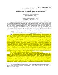
The analysis is carried out using a 1000×500 m 

computational domain while plastic deformation resulting 

from the motion of discrete dislocations is primarily 

confinedtoa10×8.6 m process window (Fig. 1a). 

The Cartesian coordinate system is also denoted in Fig. 

1(a). The portion of the computational domain outside 

the process window is discretized using a finite element 

mesh consisting of 850 plane strain quadrilateral isoparametric 

elements (CPE4 in the Abaqus notation) 

(Fig. 1b). To reduce the number of degrees of freedom 

in the boundary value problem at hand, the size of the 

elements is progressively increased with their distance 

from the process window. The process window is discretized 

using a refined mesh consisting of 48×50 

CPE4 elements, all of the same size (Fig. 1c). In accordance 

with the small-scale yielding assumption, the 

loading is applied by imposing displacements consistent 

with the elastic mode I singular field on the outside


D. Columbus, M. Grujicic / Materials Science and Engineering A000 (2001) 000–000 3 

Fig. 1. (a) The boundary value problem of a semi-infinite region subject to elastic mode I loading containing a cohesive zone at x 2=0 to enable 

crack formation and growth and a process window containing discrete dislocations; (b) and (c) the finite element meshes for the outer region and 

the ‘process window’, respectively. 

Table 1 

Material, cohesive-zone, dislocation and loading parameters used in the discrete-dislocation analysis 

Parameter Symbol Units Magnitude 

Equation Where Used 

Young’s modulus 

E 

Gpa 70 Eqs. (5), (18) and (30) 

Poisson’s ratio 

N/A 

0.33 

Eqs. (5), (6), (12), (13), (18) and (30) 

Cohesive-zone strength 

max Gpa 

0.6 

Eqs. (1) and (30) 

Cohesive-zone separation n nm 1.0 Eq. (1) 

Slip resistance 

s MPa 

3 

Eq. (2) 

Burger’s vector magnitude b nm 

0.25 

Eqs. (2), (4), (5), (12), (13), (27) and (29) 

nucl m 24 

N/A 

−2 

Source density 

10E−4 Drag coefficient 

B Pa s 

Eq. (2) 

Mean nucleation shear stress ¯ nucl MPa 

25 

N/A 

S.D. of ¯ nucl 

0.2¯ nucl MPa 

5 N/A 

Nucleation time 

Loading rate 

tnucl K I 

s 

Gpa (m) 

0.01 

N/A 

Eq. (6) 

1/2 s−1 50 

UNCORRECTED PROOF


4 


boundary of the computational domain (Fig. 1a). The 

x2=0 symmetry boundary of the computational domain 

is divided into three segments. The leftmost segment 

is modeled as the upper crack face and hence is 

subject to a traction free boundary condition. The middle 

segment is represented using cohesive-zone based interfacial 

elements while the rightmost segment of the x2=0 boundary is the plane of symmetry. Consequently, the 

middle and the rightmost segment are subject to zero 

x2-displacement and zero x1-traction boundary conditions. 

As discussed earlier, rather than employing a fracture 

criterion, crack growth is modeled using the cohesive 

zone framework [6]. The associated crack-face traction 

versus crack-face separation distance constitutive relation, 

used in the present work, is consistent with the 

exponential universal binding law [15] and is defined as: 

Un Tn(Un)=−emax exp 

n − Un (1) 

n where Tn is the normal traction, Un the normal crack-face 

separation distance and max and n are material-dependent 

cohesive-zone parameters. The cohesive-zone properties 

are assigned the same values as those used in Refs. 

[13,15] and listed in Table 1. The cohesive zone is 

modeled using two-node nonlinear spring-type interfacial 

elements whose stiffness matrix is derived using Eq. 

(1) and implemented in an Abaqus User Element Subroutine 

(UEL). Details of this procedure are given in our 

recent paper [16]. It should be noted that within the 

cohesive zone, the crack surface is defined by the top 

nodes of the interfacial elements. 

The dislocations, treated as line singularities (i.e. point 

singularities within the present two-dimensional analysis), 

are assumed to be straight, infinitely long, of the edge 

character, and to have the same magnitude of Burgers 

vector b=0.25 nm with the line direction parallel to the 

x3-axis. Furthermore, they are assumed to be associated 

with one of the two slip systems symmetrically oriented 

relative to the crack plane. The process window is 

assumed to contain a f.c.c.-like single-crystalline material 

in which the slip takes place on the {1 1 1} 1 −1 0 

family of slip systems. The f.c.c.-like single crystal is 

assumed to be oriented for symmetric double slip i.e.: x1 [−1 1 0], x2 [0 0 1], and x3 [1 1 0]. Due to the 

plane-strain condition imposed in the x3-direction, no 

slip is allowed to take place on the (1 1 1) and (1 1 −1) 

slip planes. In addition, no slip occurs in the common [1 

1 0] direction of the remaining two slip planes, (1 −1 

1) and (−1 1 1), due to the zero resolved shear stress 

in this direction under uniaxial loading in the x2-direc tion. The (1 −11)and(−111) slip planes each contain 


two more 1 −1 0 slip directions which are symmetri- 

cally aligned relative to the loading (x 2) direction. Consequently, 

plastic deformations on the slip systems based 

on these directions can be assumed to be equal in 

magnitude; therefore, the resulting net ‘effective’ slip 

directions on the (1 −1 1) and (−1 1 1) slip planes are 

[−1 1 2] and [1 −1 2]. In addition, the crack is assumed 

to reside on a {0 0 1} plane. The [−1 12]and[1−1 

2] slip directions make an angle = tan−12 5.47° with the crack plane. To be consistent with the work 

of Cleveringa et al. [12,13], an angle of =60° is used 

in the present work. 

The slip-plane spacing is set to 130b resulting in 400 

equally spaced slip planes for each slip system. At the 

beginning of the simulation, the process window is 

assumed to be free of dislocations, yet to contain a 

random distribution of dislocation sources. The density 

of the dislocation sources is given in Table 1. Details 

regarding the operation of dislocation sources, as well as 

the short-range dislocation-dislocation interactions 

which may lead to dislocation annihilation are given 

below. 

The mobility of dislocations is generally controlled by 

their interactions with both short-range obstacles which 

can be overcome by the aid of thermal activation (thermal 

obstacles) and with long-range obstacles which can not 

be thermally overcome (athermal obstacles). In pure f.c.c. 

and h.c.p. materials, where the Peierls resistance is quite 

small, forest dislocations are generally considered as the 

rate-controlling thermal obstacles and the resistance to 

dislocation motion shows a relatively weak temperature 

dependence. In b.c.c. materials, on the other hand, the 

Peierls resistance, which is substantial and increases 

rapidly with decreasing temperature, is considered to 

control the short-range dislocation interactions and the 

material strength shows a relatively strong temperature 

dependence. Large incoherent precipitates and groups of 

dislocations are typical examples of long-range athermal 

obstacles. 

In our recent work [16], the mobility of dislocations in 

b.c.c. metallic materials is studied at different temperatures. 

The results obtained show that thermal activation 

plays an important role only at temperatures a few 

hundred degrees above room temperature. Since all the 

computations in the present work are carried out for a 

f.c.c. material, at room temperature and at relatively high 

loading rates (which give rise to high stress levels), the 

effect of thermal activation is expected to be only minor 

[17,18] and a simple drag-controlled dislocation-velocity 

law can be used: 

V= effb (2) 

B 

where V is the magnitude of the dislocation velocity in 

the slip direction, eff the absolute value of the effective 

shear stress resolved on the slip plane and in the slip 

direction of the dislocation at hand, b the magnitude of 

the Burgers vector, and B is the drag coefficient. In 

contrast to the analysis of Cleveringa et al. [12,13], no 

localized obstacles to dislocation motion are considered



in the present work. Instead, a constant slip resistance 

to dislocation motion, s, is assumed to arise from the 

Peierls stress and precipitates and/or preexisting dislocation 

groups outside the process zone. In accordance 

with typical values for the slip resistance in f.c.c. materials, 

s=10 −4 ( is the shear modulus), s is set to 3 

MPa. The absolute value of the effective shear stress, 

eff, in Eq. (2) is then defined as the difference between 

the absolute value of the shear stress, , and s. When 

is less than s, the dislocation in question is assumed 

to be stationary. 

The computational analysis is carried out in an incremental 

manner by coupling a Fortran-based computer 

code, which updates the dislocation structure, with the 

commercial finite element program Abaqus/Standard 

[14], which is used to solve the resulting boundary value 

problem. Within each time step, the following computations 

are conducted. 

2.1.1. Update of the dislocation substructure 

At the beginning of a time step (time=t), the total 

(l) stress values at the position of each dislocation l, ij , 

are determined by adding the stress values arising from 

(k) all remaining dislocations kl, ˜ ij , and the stress 

values obtained at the end of the previous time step 

from the solution of the boundary value problem associated 

with the boundary conditions corrected for the 

effect of dislocations, ˆ ij, as: 

(l) (k) ij (t)= ˜ ij (t)+ˆ ij(t) (3) 

kl 

Next, the shear stress at dislocation l, acting on the slip 

plane in the glide direction, is computed as: 

(l) (t)=n (l) 

(k) (l) i ˜ ij (t)+ˆ ij(t)b j /b (4) 

kl 

(l) (l) where n i and b j are components of the unit slip plane 

normal and the Burgers vector of dislocation l, respectively. 

The magnitude of the glide velocity of dislocation 

l is then computed using Eq. (2). The direction of 

dislocation glide is based on the sign of the resolved 

shear stress, , and the sign of the dislocation’s Burgers 

vector. 

Under the assumption that the glide velocities of 

each dislocation remains constant within the time step 

of duration t, the locations of all dislocations at the 

end of the time step (time=t=t+t) could be readily 

computed. However, before dislocations are assigned 

their new positions, short-range dislocation 

interactions, which may result in annihilation and in 

nucleation of new dislocations, need to be considered. 

Should at any time within the time step the distance 


between two dislocations with opposite Burgers vectors 

gliding on the same slip plane become smaller than a 

material-dependent critical distance, L e, the two dislocations 

are annihilated. Following Cleveringa et al. 

[12,13], L e is set equal to 6b. 

As stated earlier, the process window is initially free 

of dislocations. However, as the loading proceeds, pairs 

of dislocations of the opposite Burgers vectors are 

allowed to generate on Frank–Read sources. Within 

the two-dimensional framework used in the present 

work, the Frank–Read sources are simulated as point 

sources which generate a pair of dislocations with opposite 

Burgers vectors. 

A critical shear stress for dislocation nucleation, nucl, 

is chosen at random from a Gaussian distribution with 

a mean value, ¯ nucl=25MPa, and a standard deviation 

of 0.2¯ nucl and assigned to each source. In addition, a 

fixed time period, t nucl, is selected to mimic the time 

required for a three-dimensional Frank–Read source to 

generate a new stable dislocation loop. The nucleation 

process is simulated by allowing a pair of dislocations 

to form every time the resolved shear stress acting on a 

source exceeds nucl of that source over a time period 

greater than t nucl. 

The distance between the two newly nucleated dislocations 

is set to a value L nucl at which the shear stress of 

one dislocation acting on the other dislocation is balanced 

by nucl as: 

Lnucl= E 

4(1− 2 b 

(5) 

) nucl It should be pointed out that contact interactions 

between intersecting dislocations on different slip 

planes, which give rise to the formation of sessile 

dislocation junctions of different strengths that can play 

a significant role in the kinetics of dislocation motion, 

are not considered explicitly. Nevertheless, it was observed 

that noncontact interactions of intersecting dislocations 

often yields dislocation configurations of very 

low mobility which act as dislocation locks (sessile 

junctions). 

As dislocations exit the process window they are 

retained and allowed to move and interact with other 

dislocations. The effect of loading on these dislocations 

is simplified by using the analytical mode-I stress field. 

Finally, if a dislocation glides to the crack face, it is 

removed from the material and its prior existence represented 

by a displacement step between the free surface 

and the remaining complementary dislocation. However, 

if a dislocation leaves through the closed crack 

surface, because of the assumed symmetry, its mirror 

dislocation, which prior to this event was located below 

the x1-axis and only considered indirectly through the 

symmetry boundary conditions, enters the computational 

domain along the mirror slip plane. 

2.1.2. Computation of the boundary conditions 

In the absence of dislocations, loading is accomplished 

by prescribing elastic mode I displacements on 

the outer-boundary of the computational domain as:


6 


K I I 

r 

u 1= 2 cos1−2+sin2 

2 

2 

K I I 

r 

u 2= 2 sin2−2−cos2 

(6) 

2 

2 

where 

2 2 r=x 1+x2 =tan−1x2 (7) 

x1 and the shear modulus is defined as =E/2(1+) 

and KI is the mode I stress intensity factor. 

The crack tip is taken to be initially at the origin 

(x1=x 2=0) and hence, zero-traction boundary conditions 

are prescribed along the crack face (the first 

segment of the x2=0 boundary) as: 

I I T 1(x1, x2)=T 2(x1, x2)=0 for x10; x2=0 (8) 

Along the middle segment of the x2=0 boundary, 

which is modeled as a cohesive-zone, and along the 

rightmost segment of the x2=0 boundary, the symmetry 

conditions are imposed as: 

I u 2(x1, x2)=0, I T 1(x1,x2)=0 for x10; x2=0 (9) 

When dislocations are present in the process window, 

they make contributions to the displacements and the 

tractions along the outer-boundary and the x2=0 crack 

surface, hence, the (dislocation-free) boundary conditions 

given above need to be corrected to account for 

the effect of dislocations such that the total stress and 

displacement fields agree with the boundary value problem 

shown in Fig. 1a. In the present work, the infinitemedium 

displacement and stress fields used are as 

follows: 

(l) (l) (l) 

ũ 1 (x1, x2))=cos()u 1 −sin()u 2 

(l) (l) (l) ũ 2 (x1, x2)=sin()u 1 +cos()u 2 (10) 

(l) (l) (l) ˜ 11(x1,x2)=(cos() 

11−sin() 

12) 

cos() 

(l) (l) −(cos() 12−sin() 

22) 

sin() 

(l) (l) (l) ˜ 22(x1, 

x2)=(sin() 11+cos() 

12) 

sin() 

(l) (l) +(sin() 12+cos() 

22)cos() 

(l) (l) (l) ˜ 12(x1, 

x2)=(cos() 11−sin() 

12) 

sin() 

(l) (l) +(cos() 12−sin() 

22)cos() 

(11) 

where 

(l) (l) 

b 

(l) (l) (l) x1 x2 

u 1 (x1 ,x2 )= 

2(1−) 2(r (l) ) 2+(1−) tan−1x(l) 2 

x(l)n 1 

(l) (l) (l) ũ2 (x1 , x2 ) 

= 

b 

(l) 

x2 4(1−) r (l)2 

− 1 

2 ln(r(l) ) 2 

b 2 n (1−2) (12) 

(l) (l) 2 (l) 2 b 

(l) (l) (l) x2 (3(x1 ) +(x2 ) ) 

11(x1 

, x2 )=− 

2(1−) (r (l) ) 4 

(l) (l) 2 (l) 2 b 

(l) (l) (l) x2 ((x1 ) −(x2 ) ) 

22(x1 

, x2 )= 

2(1−) (r 

n 

(l) ) 4 n 

(l) (l) 2 (l) 2 b 

(l) (l) (l) x1 ((x1 ) −(x2 ) ) 

12(x1 

, x2 )= 

2(1−) (r (l) ) 4 n (13) 

and 

(l) (l) (l) x1 (x1, x2)=cos()(x1−x 1 )+sin()(x2−x 2 ) 

(l) (l) (l) x2 (x1, x2)=−sin()(x1−x 1 )+cos()(x2−x 2 ) 

(14) 

and r (l) (l) 2 (l) 2 (l) 

=(x1 ) +(x2 ) , where x m (m=1, 2) denotes 

the location of dislocation l. As mentioned earlier, 

represents the angle that the two slip systems make with 

the crack plane (x2=0) and is set to 60°. 

The updated dislocation structure determined in Section 

2.1.1 can thus be used to compute the contributions 

of dislocations to the displacement field as: 

(l) ũi(t)= ũ i (t) 

l 

(i=1, 2) 

and to the traction fields as: 

2 

(l) T i(t)= ˜ ij (t)hj 

l j=1 

(i=1,2); hj( j=1, 2); 

are the components of the outward surface normal) 

along the outer boundary of the computational domain 

and along the crack surface and the x2=0 symmetry 

boundary. The dislocation-free elastic mode I boundary 

conditions discussed above are then corrected for the 

presence of dislocations as follows: 

1. −ũi (i=1, 2) displacements are added along the 

outer boundary; 

2. −T i(i=1, 2) tractions are added along the ‘traction-free’ 

crack surface; 

3. −ũ2 and −T 1 are prescribed along the x2=0 symmetry plane 

4. zero-displacement conditions are prescribed along 

the bottom of the cohesive zone. In addition, the 

effective stiffness and the residual forces of the 

interfacial elements are modified to account for the 

contribution of dislocations to the displacements 

and tractions along the top portion of the cohesive 

zone. A detailed account of this modification is 

given in our recent paper [16]. 

2.1.3. Solution of the boundary alue problem 

Once the ‘corrected’ boundary conditions are determined 

at the end of the time step, Abaqus/Standard is 

used to solve the boundary value problem. The computed 

stresses ˆ ij(t) are then past back to Section 2.1.1 

where they are combined with the dislocation-based 

(k) stresses k ˜ ij (t) in accordance with Eq. (3). The 

effective shear stress acting on each dislocation is next 

computed and the procedure continued as discussed in 

Section 2.1.1. 

UNCORRECTED PROOF


2.2. Nonlocal crystal-plasticity formulation 


In this section, the same plane strain mode I crack 

boundary value problem shown in Fig. 1a is analyzed. 

However, while the crack behavior is again represented 

using the cohesive zone formalism, the bulk material is 

modeled using a rate-dependent, isothermal, elastic-viscoplastic, 

finite-strain, nonlocal crystal-plasticity formulation. 

The continuum mechanics and materials science 

foundations for this model can be traced to the work of 

Anand and coworkers [19,20], and Dao and Parks [10]. 

Within the present model, the (initial) reference 

configuration is assumed to consist of a perfect, stressfree 

crystal lattice and the embedded material. The 

position of each material point in the reference configuration 

is given by its position vector X, while each 

material point in the current configuration is described 

by its position vector, x. The mapping of the reference 

configuration into the current configuration is described 

by the deformation gradient, F=x/X, a second-order 

tensor. Typically, in order to reach the current configuration, 

the reference configuration must be deformed 

both elastically and plastically. The total deformation 

gradient can be multiplicatively decomposed into its 

elastic, Fe , and plastic, Fp , parts as F=F e ·Fp .Inother 

words, the deformation of a single-crystal material 

point is considered to be the result of two independent 

atomic-scale processes: (i) an elastic distortion of the 

crystal lattice corresponding to the stretching of atomic 

bonds and; (ii) a plastic deformation associated with 

atomic plane slippage which leaves the crystal lattice 

undistorted. 

The present constitutive model is based on the following 

governing variables: (i) the Cauchy stress, T; (ii) 

the deformation gradient, F; (iii) crystal slip systems, 

labeled by integers . Each slip system is specified by a 

unit slip-plane normal n 0, and a unit vector m 0 aligned 

in the slip direction, both defined in the reference 

configuration; (iv) the plastic deformation gradient, Fp , 

with det (Fp )=1 (plastic deformation by slip does not 

give rise to a volume change); (v) the slip system 

deformation resistance s 0 which has the units of 

stress; and (vi) the density of geometrically-necessary 

dislocations associated with the slip systems , G. 

Based on the aforementioned multiplicative decomposition 

of the deformation gradient, the elastic deformation 

gradient Fe which describes the elastic 

distortions and rigid-body rotations of the crystal lattice, 

can be defined by: 

Fe =FFp−1 , det (Fe )0 (15) 

The plastic deformation gradient, Fp , on the other 


hand, accounts for the cumulative effect of shearing on 

all slip systems in the crystal. 

Since elastic stretches in metallic materials are generally 

small, the constitutive equation for stress under 

isothermal conditions can be defined by the linear 

relation: 

T*=C[Ee ] (16) 

where C is a fourth-order elasticity tensor, and E e and 

T * are, respectively, the Green elastic strain measure 

and the second Piola–Kirchoff stress measure relative 

to the intermediate, isoclinic configuration obtained 

after plastic shearing of the stress-free lattice as described 

by F p . E e and T * are respectively defined as: 

E e =(1/2){F eT F e −I}T*det(F e )F e−1 TF e−T (17) 

where I is the second order identity tensor. 

An isotropic-elasticity fourth-order tensor C, defined 

as: 

C= E 

1+ 

I+ 

1+ IIn (18) 

is used in order to ensure consistency in the elastic 

materials response in the two (discrete-dislocation and 

crystal-plasticity) formulations. I in Eq. (18) is the 

fourth-order identity tensor and denotes the tensorial 

product. 

The evolution equation for the plastic deformation 

gradient is defined by the flow rule: 

Lp =F pFp−1 = 

S0 

S0m0n0 (19) 

where Lp is the plastic velocity gradient and S0 the 

Schmid tensor. To obtain consistency in the plastic 

responses of the material in the two formulations, the 

same two slip systems discussed in the previous sections 

are used. 

The plastic shearing rate on a slip system is 

described using the following simple power-law 

relation: 

=˜ 

sign( ) (20) 

s 1/m 

where ˜ is a reference plastic shearing rate, and s 

are the resolved shear stress and the deformation resistance 

on slip system , respectively, and m is the 

material rate-sensitivity parameter. 

Since elastic stretches in metallic materials are generally 

small, the resolved shear stress on slip system can 

be defined as: 

=T* S0 (21) 

where the raised dot denotes the scalar product between 

two second order tensors. 

To complete the materials constitutive model discussed 

above, an evolution equation for the slip resistance, 

s , should be defined. Toward that end, the 

overall slip resistance of a given slip system is to have 

both a component arising from statistically stored dislocations, 

s S , and a component due to geometrically


8 


 

necessary dislocations, s G. The following function for s 

is chosen: 

s 1 

k k =[(s S) +(s G) ] k (22) 

because it ensures that s s S whenever s S sG and 

that s s G whenever s S sG . Two values of k are 

generally investigated in the literature: (a) k=1 which 

corresponds to a superposition of the contributions of 

statistically stored and geometrically necessary dislocations 

to the slip resistance; and (b) k=2 which, since 

slip resistance scales with a square root of dislocation 

density, corresponds to a superposition of the densities 

of the two types of (statistically stored and geometrically 

necessary) dislocations. In the present work however, 

only case (a), k=1, was considered. 

The evolution of the component of the slip system 

resistance associated with statistically stored dislocations 

is taken to evolve as: 

s S= h (23) 

where h is an element of the matrix which describes 

the rate of strain hardening on the slip system due to 

shearing on the coplanar (self-hardening) and noncoplanar 

(latent-hardening) slip systems . Eq. (23) is 

often used within the framework of local crystal plasticity, 

e.g. Refs. [19,20]. Following Anand and coworkers 

[19,20], the following simple form for the h element of 

the slip system hardening matrix is adopted: 

h =q h (no summation on ) 

Here, h denotes the single-slip hardening rate while 

q is a matrix describing the latent hardening behavior. 

Following Anand and coworkers [19,20], the matrix 

q and the single-slip hardening rate h are given as: 

q 1 

= 

q1=1.4 if and are coplanar slip systems 

otherwise 

(25) 

and 

h 

=h s S 

0 1− (26) 

s 1 r 

where, h 0, the initial hardening rate, s 1, the saturation 

slip resistance, and exponent r are respectively set equal 

for both slip systems (h 1 0=h 2 0, s 1 1=s 2 1). 

The component of the slip resistance arising from the 

presence of geometrically necessary dislocations, s G,is assumed to be given by the following phenomenological 

equation [10]: 

s G=cbn G (27) 

where is the shear modulus, b the magnitude of the 

Burger’s vector, c a constant (set to 0.3 in accordance 

with Ashby [21]), and n G is the density of point obstacles 

(forest dislocations) associated with geometrically 

necessary dislocations. The short-range slip resistance 

arising from these point obstacles is a strong function 

of the type of dislocation junctions formed between 

mobile dislocations on a given slip system and the 

forest dislocations. Following Franciosi and co-workers 

[22,23], the dependence of the obstacle strength on the 

type of dislocation interaction is introduced through a 

set of interaction coefficients a . Consequently, the 

density of point obstacles, n G , can be expressed as: 

n G= a G (28) 

It is well established, e.g. Ref. [10], that the density of 

geometrically-necessary dislocations scales with the 

Nye’s dislocation tensor, the tensor which is a measure 

of the tensorial curl of FP . Following the procedure 

proposed by Dao and Parks [10], which is briefly 

overviewed in the Appendix, an evolution equation for 

the density of geometrically necessary dislocations associated 

with each slip system, under the plane-strain 

condition, is derived as: 

1 d 

G= +F21 )] 

[ bp 0(3) dx2 P (F 11n 

0(1) 

− d 

[ 

dx1 P P (F 12n 

0(1) +F22n 

0(2) 

P n 0(2) 

)] (29) 

where n 0(1) and n 0(2) are components of the slip plane 

normal n 0, and p 0(3) is a component of p 0, a vector 

defined as p 0=m 0×n 0. The geometrically necessary 

dislocations are of the edge character, with their line 

directions parallel to the x3-axis and their Burgers 

vectors collinear with the corresponding slip direction 

m 0. 

The stress strain relationship, Eq. (16), the flow rule, 

Eq. (20), and the evolution equations for the slip resistance 

due to statistically stored dislocations, Eq. (23), 

and for the geometrically-necessary dislocations, Eq. 

(27), constitute the non-local crystal-plasticity material 

constitutive model. The integration of the model along 

the loading path is carried out within the User Material 

Subroutine (UMAT) of Abaqus/Standard. With the 

exception of the density of geometrically-necessary dislocations, 

all other material state variables are integrated 

using a forward Euler approach. Since the 

integration of the density of geometrically necessary 

dislocations requires the computation of the gradient of 

state variables, which in turn depends on the material 

state at surrounding integration points, a backward 

Euler integration scheme was used to update G. Since 

the same integration scheme has been applied in a 

number of our recent studies, e.g. Ref. [24] it will not be 

discussed here. 

UNCORRECTED PROOF



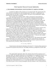
Fig. 2. The variation of the normalized mode I stress intensity factor 

with crack extension for the discrete dislocation analysis (Discrete 

Dislocation) and two crystal plasticity analyses (Model-I and Model- 

II). 

3. Results and discussion 

3.1. Discrete-dislocation analysis 

In this section, selected results are shown for the 

discrete-dislocation analysis of plane-strain mode I 

crack growth. The material, cohesive-zone, dislocation, 

and loading parameters used in this analysis are summarized 

in Table 1. 

The variation of crack extension with the applied 

stress intensity factor (the curve denoted ‘Discrete Dislocation’) 

is shown in Fig. 2. The stress intensity factor 

is normalized with respect to its critical value corresponding 

to unstable crack growth without any dislocation 

activity, K I0, defined as [25]: 

KI0= En 1− 2 

(30) 

where n=e max n is the work of separation. 

The results shown in Fig. 2 indicate that the crack 

begins to extend at the normalized stress intensity factor 

of K I/K I0=1.10. The initial crack extension (up to 

ca. 0.3 m) is characterized with a very slow rise in the 

normalized stress intensity factor. This regime of crack 

extension is followed by one in which the normalized 

stress intensity factor rises very steeply. When K I/K I0 

reaches a value of approximately 2.0, the crack extension 

regime characterized by a slow increase in K I/K I0 

The dislocation structure, a contour plot of the total 

normal stress, 22, and the distorted finite element mesh 

in the process window at the onset of crack extension 

are shown in Fig. 3a–c, respectively. 

To distinguish between positive and negative dislocations 

residing on the two slip systems shown in Fig. 3a, 

solid and open symbols are used to represent dislocations 

on the =60° and =120° slip systems, respectively; 

while, delta and gradient symbols denote, 

respectively, positive and negative dislocations on both 

slip systems. The results shown in Fig. 3a can be 

summarized as follows: 

1. the dislocation activity is localized on slip systems 

originating from the region near the crack tip; 

2. a substantially larger number of dislocations are 

associated with the =60° slip system than with the 

=120° slip system; 

3. there is some evidence of dislocation polarization. 

For example, mostly negative dislocations are found 

near the crack tip on both slip systems. Conversely, 

near the outer-boundary of the process window the 

dislocations are mostly of the positive sign. 

In the total 22 stress field contour plot shown in Fig. 

3b, the darkest shade of gray is used to denote the 

highest positive stress values. It should be noted that 

despite the fact that the dislocation-based 22 stress is 

singular, no stress singularities are present in Fig. 3b 

since the stresses had to be extrapolated to the nodal 

points for plotting purposes. The results shown in Fig. 

3b can be summarized as follows: 

1. the stress field is roughly partitioned into three 

regions, with little stress variation within each region. 

The region ahead of the crack tip is characterized 

by relatively large tensile 22 stress, while the 

region in the crack wake contains small (mostly 

negative) 22 stress values; 

2. at many places 22 is dominated by the dislocationbased 

˜ 22 stress which gives rise to small (diamondshaped) 

regions of significantly different value of 22 than that of its surroundings. 

The distorted finite element mesh in the process 

window of the computational domain at the onset of 

crack extension is shown in Fig. 3c. To enhance clarity, 

a magnification factor of 30 is applied to the nodal 

displacements. The location of the crack tip is denoted 

by an arrow. A careful examination of Fig. 3c reveals 

the presence of two not fully developed deformation 

bands emanating from the crack tip and aligned with 

the respective slip systems. These bands are clearly the 

result of the localized dislocation structure observed in 

Fig. 3a. 

The dislocation structure, the contour plot of the 

total normal stress, 22, and the distorted finite element 

mesh in the process window at the normalized stress 

intensity factor KI/KI0=1.48 are shown respectively in 

Fig. 4a–c. Based on the results shown in Fig. 2, at 


resumes. This period of crack growth is again pro- 

ceeded by the regime within which the crack-extension 

resistance (change of K I/K I0 per change in crack extension) 

is relatively high.


10 


K I/K I0=1.48, the crack extension is characterized by a 

high fracture resistance (i.e. K I/K I0 increases sharply 

with crack extension). 

A comparison of the results shown in Fig. 3a and 

Fig. 4a indicates that the density of dislocations on 

both slip systems has increased while their activity 

remains localized within two broad bands emanating 

from the crack tip region. 

By comparing the results shown in Fig. 3b and Fig. 

4b the following observations can be made: 

1. the three 22 stress regions observed at the onset of 

crack extension are maintained at higher values of 

K I/K I0; 

2. due to a large density of dislocations at higher 

K I/K I0 values, the dislocations’ effects on the 22 

stress field become more pronounced, Fig. 4b; 

3. the region of the highest tensile stress ahead of the 

crack tip, responsible for crack advance (the region 

denoted by the darkest shade of gray), is substantially 

reduced at K I/K I0=1.48, Fig. 4b, in comparison 

to that at the onset of crack extension, Fig. 3b. 

This finding is fully consistent with the results 

shown in Fig. 2, which indicate a sharp increase in 

K I/K I0. This implies that higher loading is needed to 

extend the region of maximum tensile stress ahead 

of the crack tip before significant crack extension 

can take place. 

A comparison of the results shown in Fig. 3c and 

Fig. 4c indicates that as loading proceeds the deformation 

bands become more developed. As in the case of 

Fig. 3c, the position of the crack tip is denoted by an 

arrow. 

The dislocation structure, a contour plot of the total 

normal stress, 22, and the distorted finite element mesh 

in the process window at the normalized stress intensity 

factor K I/K I0=2.10 are shown in Fig. 5a–c, respectively. 

At this level of K I/K I0, the crack extends relatively 

easily (i.e. the K I/K I0 versus a curve has a small 

slope, Fig. 2). 

Comparison of the results shown in Fig. 5a with their 

counterparts shown in Fig. 3a and Fig. 4a indicates that 

dislocation density increases fairly monotonically with 


Fig. 3. (a) The dislocation structure; (b) the 22 stress contour plot and (c) the deformed finite element mesh for the discrete dislocation analysis 

at the onset of crack extension (K I/K I0=1.10, arrows indicate position of crack tip).



Fig. 4. (a) The dislocation structure; (b) the 22 stress contour plot 

and (c) the deformed finite element mesh for the discrete dislocation 

analysis at the normalized stress intensity factor K I/K I0=1.48 (arrows 

indicate position of crack tip). 

The 22 stress contour plot shown in Fig. 5b displays 

the three familiar stress regions, and, as a consequence 

of a higher dislocation density, a more pronounced 

contribution from ˜ 22. The main change in the stress 

field, however, is the establishment of a larger high 

tensile stress region ahead of the crack tip. The lower 

crack resistance at this value of K I/K I0 appears to be 

related to the presence of this stress region. 

The deformed finite element mesh shown in Fig. 5c 

indicates a larger crack opening displacement in the 

crack wake. However, very little change can be observed 

in the shape of the crack tip in comparison to 

the one shown in Fig. 4c. This finding is consistent with 

the fact that between K I/K I0=1.48 and K I/K I0=2.10, 

there is very little crack extension, thus, the imposed 

loading is mainly absorbed by dislocation-based deformation 

of the material. 

3.2. Nonlocal crystal-plasticity analysis 

In this section selected results are shown for the 

crystal-plasticity analysis of plane strain mode I crack 

growth. The cohesive-zone and the loading parameters 

are identical to the ones listed in Table 1. As far as the 

crystal-plasticity parameters are concerned, it was not 

possible to determine a set of parameters which would 

replicate the KI/KI0 versus a resistance curve obtained 

using the discrete-dislocation approach, Fig. 2. The 

KI/KI0 versus a curves obtained using the crystal-plasticity 

analysis show a monotonically increasing normalized 

stress intensity factor, KI/KI0, with a (as opposed 

to having a step-like behavior obtained in the discretedislocation 

analysis). In addition, the overall slope of 

the KI/KI0 versus a curves obtained using the crystalplasticity 

analysis is generally quite small in comparison 

to the overall slope of the corresponding KI/KI0 versus 

a curve obtained using the discrete-dislocation approach. 

To overcome this problem, two sets of crystalplasticity 

parameters were assessed (Table 2). The first 

set gives rise to a KI/KI0 versus a response which best 

matches the initial portion of the KI/KI0 versus a curve 

obtained using the discrete-dislocation analysis. The 

second set of crystal-plasticity parameters is determined 

in such a way that the KI/KI0 versus a response best 

matches the overall KI/KI0 versus a response obtained 

using the discrete-dislocation approach. The resulting 

crystal-plasticity based KI/KI0 versus a curves are denoted 

in Fig. 2 as Model-I and Model-II, respectively. 

The equivalent plastic strain, normal, 22, stress contour 

plot, and the deformed finite element mesh at 

KI/KI0=1.18, the onset of crack extension for the 

Model-I nonlocal crystal-plasticity analysis, are shown 

in Fig. 6a–c, respectively. Again, the regions associated 

with the largest values of the equivalent plastic strain 

and 22 stress are denoted by the darkest shade of gray 

in Fig. 6a and b. 


K I/K I0. However, no major changes in the width of 

dislocation bands and the extent of dislocation polarization 

can be observed at high values of K I/K I0.


12 


The results shown in Fig. 6a indicate that plastic 

deformation is localized into two deformation bands, 

emanating from the region surrounding the crack tip. 

The deformation band associated with the =60° slip 

system is more developed and contains the region of 

highest equivalent plastic strain. This finding is consis- 

tent with the dislocation structure at a comparable 

K I/K I0 level, Fig. 3a. 

The contour plot of the 22 stress shown in Fig. 6b 

indicates that the stress field around the crack tip is 

partitioned into three regions, each characterized by a 

different level of average stress. The region ahead of the 

Fig. 5. (a) The dislocation structure; (b) the 22 stress contour plot and (c) the deformed finite element mesh for the discrete dislocation analysis 

at the normalized stress intensity factor K I/K I0=2.10 (arrows indicate position of crack tip). 

Table 2 

Material parameters used in the nonlocal crystal-plasticity analyses (Model-I and Model-II) 

Parameter 

Symbol Units Magnitude (Model-I) Magnitude (Model-II) Equation where used 

s 0.001 

0.010 

−1 Reference plastic shearing rate 

0 

Eq. (20) 

Material rate sensitivity parameter m N/A 0.01 0.01 Eq. (20) 

Initial local slip resistance sS,0 MPa 11.0 

11.0 

Eq. (23) 

Latent hardening parameter 

ql N/A 1.4 1.4 

Eq. (25) 

Initial local hardening rate h MPa 380 

100 

0 

Eq. (26) 

Local saturation slip resistance s MPa 

1 160 160 Eq. (26) 

Local hardening exponent r N/A 1.2 

1.2 

Eq. (27) 

Ashby’s constant c N/A 0.3 0.3 Eq. (28) 

Interaction coefficient a11=a 22 N/A 0.45 

0.20 

Eq. (29) 

Interaction coefficient 

a12=a 21 N/A 0.45 0.20 Eq. (29) 

UNCORRECTED PROOF



Fig. 6. (a) The equivalent plastic strain contour plot; (b) the 22 stress 

contour plot and (c) the deformed finite element mesh for the 

nonlocal crystal plasticity (Model-I) analysis at the onset of crack 

extension (K I/K I0=1.18, arrows indicate position of crack tip). 

addition, the stress levels in the corresponding three 

regions are comparable for the two types of analyses. A 

comparison of the distorted finite element mesh resulting 

from the crystal-plasticity analysis, Fig. 6c, with the 

corresponding mesh resulting from the discrete-dislocation 

analysis, Fig. 3c, indicates very similar crack profiles 

in the two cases. However, the deformation bands 

observed in Fig. 3c, can not be readily identified in Fig. 

6c. 

To show the role of the nonlocal crystal-plasticity 

phenomenon on mode I crack growth behavior, the 

equivalent plastic strain, the normal, 22, stress contour 

plot, and the distorted mesh obtained from a crystal-plasticity 

analysis based on Model-I parameters, but with the 

nonlocal parameters (c, a0 and a1) turned off, at the same 

level of stress intensity factor as in Fig. 6a–c (KI/KI0= 1.18), are shown in Fig. 7a–c. This analysis is referred 

to as a local crystal-plasticity analysis. 

The main differences in the distribution of equivalent 

plastic strain in local (Fig. 7a) and nonlocal (Fig. 6a) 

crystal-plasticity analyses can be summarized as follows: 

1. higher values of equivalent plastic strain are observed 

in the local-plasticity case and the highest 

plastic-strain region is located at the crack tip. In 

the nonlocal crystal-plasticity case, the highest plastic-strain 

region is slightly removed from the crack 

tip; 

2. the plastic strain bands, while well formed in both 

cases, appear to be narrower in the local-plasticity 

case. 

A comparison of the local, Fig. 7b, and nonlocal, 

Fig. 6b, 22 stress distributions indicates that while the 

distributions are quite similar, ca. 8% higher tensile 

stress levels are attained in the nonlocal crystal-plasticity 

case. 

A comparison of the local, Fig. 7c, and nonlocal, 

Fig. 6c, deformed finite element meshes indicates significant 

differences in the crack profile especially near 

the crack tip. In the local crystal-plasticity case, the 

crack tip is quite blunted and no crack advance is 

observed. In sharp contrast, the crack tip is considerably 

sharp and crack extension is observed in the case 

of nonlocal crystal plasticity. 

The equivalent plastic strain, the normalized 22 stress contour plot, and the deformed finite element 

mesh at the onset of crack extension (KI/KI0=1.53) for 

the Model-II nonlocal crystal-plasticity analysis are 

shown in Fig. 8a–c, respectively. 

A comparison of the equivalent plastic strain distributions 

obtained using Model-II (Fig. 8a) and Model-I 

(Fig. 6a) nonlocal crystal-plasticity analyses indicates 

that higher plastic strain levels are attained in the 

former case. In addition, the highest plastic strain region 

in the case of Model-II is located at the crack tip. 

These findings are consistent with the fact that in order 

to delay the onset of crack extension in the Model-II 


crack tip is associated with the highest tensile stress 

values while the region behind the crack tip contains 

low-magnitude primarily negative 22 stress values. 

These observations are fully consistent with the ones 

made during the discrete-dislocation analysis, Fig. 3b. In


14 


analysis, the nonlocal effects were reduced. The similarities 

between the results shown in Fig. 8a with those 

shown in Fig. 7a suggest that nonlocal crystal-plasticity 

effects play a smaller role in Model II. 

A comparison of Model-II (Fig. 8b) and Model-I 

(Fig. 6b) normal, 22, stress distributions indicates that 

while the two stress fields are very similar, and in 

particular, the shapes of the regions of highest tensile 

stress are almost identical, somewhat (ca. 5%) lower 

stress levels are observed in the case of the Model-II 



contour plot and (c) the deformed finite element mesh for the local 

crystal plasticity analysis at the onset of crack extension (KI/KI0= 1.18, arrows indicate position of crack tip). 



nonlocal crystal plasticity (Model-II) analysis at the onset of crack 

extension (K I/K I0=1.53, arrows indicate position of crack tip).



crystal-plasticity analysis. This finding can be attributed 

to the aforementioned less pronounced role of the 

nonlocal effects in the Model-II analysis. 

The crack profile, in Fig. 8c, is more blunted in 

comparison to that for Model-I, Fig. 6c. This is another 

indication of the less pronounced role of nonlocal 

crystal-plasticity effects in the former case. 

Above, results shown in Fig. 6 and Fig. 8 were used 

to compare the corresponding fields and deformed finite 

element meshes from Model-I and Model-II crystalplasticity 

analyses at the respective onsets of crack 

extension. Therefore, the K I/K I0 values where different 

in the two cases. The results shown in Fig. 9a–c are 

used to show the effect of nonlocal crystal-plasticity 

parameters at the same level of K I/K I0. That is, the 

results shown in Fig. 9a–c are obtained using the 

Model-I crystal-plasticity analysis at a level of the stress 

intensity factor of 1.53 (level of K I/K I0 at which crack 

advance begins for the Model-II analysis). 

The equivalent plastic strain distribution results 

shown in Fig. 9a can be summarized as follows: 

1. The deformation band associated with the =60° 

slip system broadens as the crack extends. Band 

broadening takes place mainly in the direction of 

crack extension. 

2. The highest plastic strain region remains removed 

from the crack tip, while the plastic deformation 

band as a whole, expands and increases in 

magnitude. 

3. The region just ahead of the crack tip is characterized 

by low plastic strain values. It appears that the 

crack tip is advancing into an elastic region. 

The normal, 22, stress contour plot shown in Fig. 9b 

indicates that the stress field possesses the same basic 

features previously identified in Fig. 6b, Fig. 7b, and 

Fig. 8b. The new feature of the stress field shown in 

Fig. 9b is the lateral movement of the region of maximum 

tensile stress with the crack tip. 

The deformed mesh shown in Fig. 9c, as well as the 

one shown in Fig. 7c indicate that the crack profile 

remains sharp as it advances. Again, no well-defined 

deformation bands can be observed. 

3.3. Comparison of discrete-dislocation and 

crystal-plasticity analyses 

A comparison of the corresponding results shown in 

Figs. 3–9 suggests that the dislocation/plastic strain 

and 22 stress fields as well as distorted finite element 

meshes and crack profiles obtained using the discretedislocation 

and crystal-plasticity analyses are quite 

comparable. Nevertheless, some significant differences 

can be identified: 

1. the 22 stress fields, which in both analyses consists 

of three well defined regions, can be locally very 

different due to the ˜ 22 stress contribution in the 

discrete-dislocation analysis. This is particularly 

pronounced within the two deformation bands emanating 

from the crack tip region which contain high 

densities of dislocations; 




nonlocal crystal plasticity (Model-I) analysis at the normalized stress 

intensity factor KI/KI0=1.53 (arrows indicate position of crack tip).


16 


2. localization of plastic deformation in the form of 

deformation bands emanating from the crack tip is 

substantially more pronounced in the discrete-dislocation 

case (e.g. Fig. 4c) than in the crystal-plasticity 

case (e.g. Fig. 8c). This difference can be readily 

explained. In the crystal-plasticity analysis, while 

plastic deformation takes place on specific crystallographic 

slip systems, the systems are distributed in a 

continuous manner throughout the material. Consequently, 

plastic deformation varies continuously 

throughout the material. In sharp contrast, in the 

discrete-dislocation analysis, the same crystallographic 

slip systems are represented in a discrete 

fashion. Consequently, plastic deformation is the 

result of the nucleation and motion of discrete dislocations 

on discrete slip planes; 

3. while the overall (stress and strain) fields which 

resulted from the discrete-dislocation and the nonlocal 

crystal-plasticity analyses are qualitatively (and 

to a good extent quantitatively) similar, the global 

(stress intensity versus crack extension) responses 

show significant differences. Primarily, the response 

obtained using the crystal-plasticity analysis is 

monotonic, while the one resulting from the discrete-dislocation 

analysis has a step-wise character. 

In addition, the overall slopes of the K I/K I0 versus 

a curves differ in the two cases by a factor of three 

to four which can give rise to a substantial difference 

in the stress intensity factor at the crack extensions 

significantly larger than the ones analyzed in 

the present work. These differences can be attributed 

to the fact that within the discrete-dislocation 

approach, the dislocation structure is 

undergoing a continuous evolution. Consequently, 

various dislocation configurations with greatly different 

net stress and displacement fields are being 

generated. Some of these configurations impede 

crack extension resulting in a steep K I/K I0 versus a 

response. Others, on the other hand interfere with 

plastic deformation promoting crack extension. In 

the case of crystal plasticity, due to the continuum 

nature of crystallographic slip, the fields and the 

overall material response evolve only in a continuous 

manner. 

4. Conclusions 

Based on the results obtained in the present work, 

the following main conclusions can be drawn: (1) Mode 

I fracture problem in the presence of crystallographic 

sip can be analyzed in a consistent manner using both 


discrete-dislocation and continuum crystal-plasticity 

formulations. Within both formulations, the cohesive 

zone approach can be used to represent the force-displacement 

crack constitutive behavior. (2) When com- 

pared at comparable levels of the applied stress 

intensity factor, the dislocation/strain and stress fields, 

as well as distorted meshes and crack profiles are quite 

comparable for the two approaches. The observed differences 

in these fields can be readily attributed to the 

discrete nature of dislocations and to the discrete nature 

of slip systems in the discrete-dislocation approach. 

(3) The main difference in the results obtained using the 

two formulations pertains to the global stress intensity 

versus crack extension response. The continuum-nature 

of the crystal-plasticity analysis yields a monotonic 

K I/K I0 versus a response. In sharp contrast, the discrete 

nature of dislocations and their sources, as well as 

the interaction between dislocations and the advancing 

crack tip, gives rise to a step-like K I/K I0 versus a 

behavior. 

5. Uncited references 

[26]. 

Acknowledgements 

The material presented here is based on work supported 

by the National Science Foundation, Grant 

Numbers DMR-9906268 and CMS-9531930 and by the 

US Army Grant Number DAAH04-96-1-0197. The authors 

are indebted to Drs Bruce A. MacDonald and 

Daniel C. Davis of NSF and Dr David M. Stepp of 

ARO for the continuing interest in the present work. 

The help of Dr Erik van der Giessen in providing the 

preprints of his work and in clarifying some aspects of 

the computational procedure is greatly appreciated. 

The authors also acknowledge the support of the Office 

of High Performance Computing Facilities at Clemson 

University. 

Appendix A. Derivation of an evolution equation for 

the density of geometrically necessary dislocations. 

If dX represents an infinitesimal vector connecting 

two material points in the reference configuration, then 

its image in the intermediate configuration obtained 

after plastic deformation is given as: 

dY=F p dX (A1) 

Then, for an infinitesimal surface S in the reference 

configuration which has a unit normal r 0 and is enclosed 

counterclockwise by a circuit C, the total Burgers 

vector content of all the dislocations piercing the 

area S can be evaluated using the standard right-hand 

Burgers circuit. The image of C in the intermediate 

configuration obtained after plastic shearing of the



crystal lattice, C 1 , is generally an open contour, and 

hence, the line integral C 1dY defines the closure failure. 

Since the total Burgers vector B completes the circuit 

C 1 , it can be defined as: 

B=− dY=− FpdX (A2) 

C 1 

C 

Eq. (A2) can be transformed into: 

B=− (×F pT ) Tr0 dS= r0 dS (A3) 

S 

using a generalized Stokes theorem. in Eq. (A2) is the 

so-called Nye’s tensor [26], and is defined as the tensorial 

curl of F p as: 

−(×F pT ) T (A4) 

The material derivative of the Nye’s tensor can be 

defined as: 

−(×F pT ) T (A5) 

which through the use of Eq. (19), becomes: 

=−[×(LpFp ) T ] T =−× 

m pnTT 

0n0 F 

(A6) 

Next, the portion of associated with activity of slip 

system is defined as: 

−{×[( m 0 n0 )F p ] T } T 

S 

=−m 0 [×( F pT n0 )] (A7) 

Thus 

= 

 

(A8) 

Next, a phenomenological equation for is defined as 

follows. is assumed to scale with the accumulation 

rate of three sets of geometrically necessary dislocations 

all with Burgers vectors in the m0 direction: (a) a set of 

screw dislocations with tangent vector in the m0-direc tion; (b) a set of edge dislocations with tangent vector 

in the x3-direction; and (c) a set of edge dislocations 

with tangent vector in the n0-direction. Hence, for a 

cubic lattice with a common Burgers vector magnitude, 

b, can be written as: 

=m0b( G m0+ G p0+ G n0) (A9) 

(s ) 

(e )1 

(e )2 

where G , G , and G are the accumulation 

(s ) (e )1 

(e )2 

rates of density of the three aforementioned sets of 

geometrically necessary dislocations, respectively. A 

comparison of the second Eq. (A7) and Eq. (A9) yields: 


−×( F pT n 0 )=b( G (s)m 0 + G (e)1p 0 + G (e)2n 0 ) (A10) 

It can be easily shown that for in-plane-strain deformation, 

(F P 13=F P 23=F P 31=F P 32=0, F P 33=1), Eq. (A10) 

yields: 

G (s)=0, G (e)2=0 

and 

G (e )1 

= 1 

d 

[ P P (F 11n 

0(1) +F21n 

0(2) )] 

bp 0(3) dx2 − d 

[ 

dx1 P P (F 12n 

0(1) +F22n 

0(2) )] (A11) 

Eq. (A11) is an evolution equation for the density of 

geometrically necessary dislocations and is used in Section 

2.2 to evaluate the non-local contribution to the 

slip resistance. 

References 

[1] G.R. Irwin, Fracture, in: S. Flugge (Ed.), Encyclopedia of 

Physics, vol. 6, Springer New York, New York, 1958, pp. 

551–590. 

[2] L.B. Freund, The mechanics of dislocations in strained-layer 

semiconductor-materials, Adv. Appl. Mech. 30 (1994) 1–66. 

[3] V. Tvergaard, J.W. Hutchinson, The relation between crack 

growth resistance and fracture process parameters in elastic-plastic 

solids, J. Mech. Phys. Solids 40 (1992) 1377–1397. 

[4] I.-H. Lin, R. Thomson, Cleavage, dislocation emission, and 

shielding for cracks under general loading, Acta Metall. 34 

(1986) 187–206. 

[5] V. Shastry, P.M. Anderson, R. Thomson, Nonlocal effects of 

existing dislocations on crack-tip emission and cleavage, J. 

Mater. Res. 9 (1994) 1–16. 

[6] A. Needleman, A continuum model for void nucleation by 

inclusion debonding, J. Appl. Mech. 54 (1987) 525–531. 

[7] N.A. Fleck, J.W. Hutchinson, Strain gradient plasticity, Adv. 

Appl. Mech. 33 (1997) 295–361. 

[8] N.A. Fleck, G.M. Muller, M.F. Ashby, J.W. Hutchinson, Strain 

gradient plasticity: theory and experiment, Acta Metall. Mater. 

42 (1994) 475–487. 

[9] A. Acharya, J.L. Bassani, Incompatibility and crystal plasticity, 

J. Mech. Phys. Solids (1998) (in press). 

[10] H. Dao, Parks, Geometrically necessary dislocation density in 

continuum plasticity theory, FEM implementation and application, 

PhD Thesis, MIT, August 1997. 

[11] Z. Suo, C.F. Shih, A.G. Varias, A theory for cleavage cracking 

in the presence of plastic flow, Acta Metall. Mater. 41 (1993) 

1551–1557. 

[12] H.H. M. Cleveringa, E. van der Giessen, A. Needleman, A 

discrete dislocation analysis of mode I crack growth, J. Mech. 

Phys. Solids (in press) 

[13] H.H. M. Cleveringa, E. van der Giessen, A. Needleman, A 

discrete dislocation analysis of rate effects in mode I crack 

growth, Mater. Sci. Eng. (in print). 

[14] ABAQUS Theory Manual, Version 5.8, Habbilt, Karlsson, and 

Soreassen, Providence, RI, 1999. 

[15] J.H. Rose, J. Ferrante, J. Smith, Universal binding energy curves 

for metals and bimetallic interfaces, Phys. Rev. Lett. 47 (1981) 

675–678. 

[16] M. Grujicic, D. Columbus, Discrete-dislocation analysis of ductile-to-brittle 

transition in BCC-like metallic materials, J. Mater. 

Sci. (2000) (in print). 

[17] A.S. Krausz, H.E. Eyring, Deformation Kinetics, Wiley, New 

York, 1975. 

[18] V.F. Kocks, A.S. Argon, M.F. Ashby, Thermodynamics and 

Kinetics of Slip, Pergamon, London, 1975 in Progress in Materials 

Science.


18 


[19] S.R. Kalidindi, C.A. Bronkhorst, L. Anand, J. Mech. Phys. 

Solids 40 (1992) 537–569. 

[20] C.A. Bronkhorst, S.R. Kalidindi, L. Anand, Phil. Trans. R. Soc. 

Lond. A341 (1992) 443–477. 

[21] M.F. Ashby, The deformation of plastically non-homogeneous 

materials, Phil. Mag. 21 (1970) 399–424. 

[22] P. Franciosi, M. Berveiller, A. Zaoui, Latent hardening in copper 

and aluminum single crystals, Acta Metall. 28 (1980) 273– 

283. 

[23] P. Franciosi, A. Zaoui, Multislip in FCC crystals: a theoretical 

approach compared with experimental data, Acta Metall. 30 

(1982) 1627–1637. 

[24] M. Grujicic, Y. Zhang, J. Mater. Sci. 34 (1999) 1419–1437. 

[25] J.R. Rice, A path independent integral and the approximate 

analysis of strain concentration by notches and cracks, J. Appl. 

Mech. 35 (1968) 379–386. 

[26] J.F. Nye, Some geometrical relations in dislocated crystals, Acta 

Metall. 1 (1953) 153–162. 


.

A comparative discrete-dislocation/nonlocal crystal-plasticity

You also want an ePaper? Increase the reach of your titles

Delete template?

Save as template?