Tutorial slides (PDF) - Clemson University

Python for Scientific and High 

Performance Computing 

SC09 

Portland, Oregon, United States 

Monday, November 16, 2009 1:30PM - 5:00PM 

http://www.cct.lsu.edu/~wscullin/sc09python/

Introductions 

Your presenters: 

William R. Scullin 

wscullin@alcf.anl.gov 

James B. Snyder 

jbsnyder@northwestern.edu 

Nick Romero 

naromero@alcf.anl.gov 

Massimo Di Pierro 

mdipierro@cs.depaul.edu

Overview 

We seek to cover: 

Python language and interpreter basics 

Popular modules and packages for scientific applications 

How to improve performance in Python programs 

How to visualize and share data using Python 

Where to find documentation and resources 

Do: 

Feel free to interrupt 

the slides are a guide - we're only successful if you learn 

what you came for; we can go anywhere you'd like 

Ask questions 

Find us after the tutorial

About the Tutorial Environment 

Updated materials and code samples are available at: 

http://www.cct.lsu.edu/~wscullin/sc09python/ 

we suggest you retrieve them before proceeding. They should 

remain posted for at least a calendar year. 

You should have login instructions, a username and password 

for the tutorial environment on the paper on your slip. Accounts 

will be terminated no later than 6:30PM USPT today. Do not 

leave any code or data on the system you would like to keep. 

Your default environment on the remote system is set up for 

this tutorial, though the downloadable live dvd should provide a 

comparable environment.

1. Introduction 

Introductions 

Tutorial overview 

Why Python and why in scientific and 

high performance computing? 

Setting up for this tutorial 

2. Python basics 

Interpreters 

data types, keywords, and functions 

Control Structures 

Exception Handling 

I/O 

Modules, Classes and OO 

3. SciPy and NumPy: fundamentals and 

core components 

Outline 

4. Parallel and distributed programming 

5. Performance 

Best practices for pure Python + 

NumPy 

Optimizing when necessary 

7. Real world experiences and techniques 

8. Python for plotting, visualization, and 

data sharing 

Overview of matplotlib 

Example of MC analysis tool 

9. Where to find other resources 

There's a Python BOF! 

10. Final exercise 

11. Final questions 

12. Acknowledgments

Dynamic programming language 

Interpreted & interactive 

Object-oriented 

Strongly introspective 

Provides exception-based error handling 

Comes with "Batteries included" (extensive standard 

libraries) 

Easily extended with C, C++, Fortran, etc... 

Well documented (http://docs.python.org/)

Why Use Python for Scientific 

Computing? 

"Batteries included" + rich scientific computing ecosystem 

Good balance between computational performance and 

time investment 

Similar performance to expensive commercial solutions 

Many ways to optimize critical components 

Only spend time on speed if really needed 

Tools are mostly open source and free (many are MIT/BSD 

license) 

Strong community and commercial support options. 

No license management

Science Tools for Python 

Large number of science-related modules: 

General 

NumPy 

SciPy 

GPGPU Computing 

PyCUDA 

PyOpenCL 

Parallel Computing 

PyMPI 

Pypar 

mpi4py 

Wrapping 

C/C++/Fortran 

SWIG 

Cython 

ctypes 

Plotting & Visualization 

matplotlib 

VisIt 

Chaco 

MayaVi 

AI & Machine Learning 

pyem 

ffnet 

pymorph 

Monte 

hcluster 

Biology (inc. neuro) 

Brian 

SloppyCell 

NIPY 

PySAT 

Molecular & 

Atomic Modeling 

PyMOL 

Biskit 

GPAW 

Geosciences 

GIS Python 

PyClimate 

ClimPy 

CDAT 

Bayesian Stats 

PyMC 

Optimization 

OpenOpt 

Symbolic Math 

SymPy 

Electromagnetics 

PyFemax 

Astronomy 

AstroLib 

PySolar 

Dynamic Systems 

Simpy 

PyDSTool 

Finite Elements 

SfePy 

For a more complete list: http://www.scipy.org/Topical_Software

Please login to the Tutorial Environment 

Let the presenters know if you have any issues. 

Start an iPython session: 

santaka:~> wscullin$ ipython 

Python 2.6.2 (r262:71600, Sep 30 2009, 00:28:07) 

[GCC 3.3.3 (SuSE Linux)] on linux2 

Type "help", "copyright", "credits" or "license" for more 

information. 

IPython 0.9.1 -- An enhanced Interactive Python. 

? -> Introduction and overview of IPython's features. 

%quickref -> Quick reference. 

help -> Python's own help system. 

object? -> Details about 'object'. ?object also works, ?? prints 

more. 

In [1]:

Python Basics 

Interpreter 

Built-in Types, keywords, functions 



I/O 

Modules, Classes & OO

Interpreters 

CPython Standard python distribution 

What most people think of as "python" 

highly portable 

http://www.python.org/download/ 

We're going to use 2.6.2 for this tutorial 

The future is 3.x, the future isn't here yet 

iPython 

A user friendly interface for testing and debugging 

http://ipython.scipy.org/moin/

Other Interpreters You Might See... 

Unladen Swallow 

Blazing fast, uses llvm and in turn may compile! 

x86/x86_64 only really 

Sponsored by Google 

http://code.google.com/p/unladen-swallow/ 

Jython 

Python written in Java and running on the JVM 

http://www.jython.org/ 

performance is about what you expect 

IronPython 

Python running under .NET 

http://www.codeplex.com/IronPython 

PyPy 

Python in... Python 

No where near ready for prime time 

http://codespeak.net/pypy/dist/pypy/doc/

CPython Interpreter Notes 

Compilation affects interpreter speed 

Distros aim for compatibility and as few irritations as 

possible, not performance 

compile your own or have your systems admin do it 

same note goes for most modules 

Regardless of compilation, you'll have the same 

bytecode and the same number of instructions 

Bytecode is portable, binaries are not 

Linking against shared libraries kills portability 

Not all modules are available on all platforms 

Most are not OS specific, 90% are available everywhere 

x86/x86_64 is still better supported than most

A note about distutils and building 

modules 

Unless your environment is very generic (ie: a major linux 

distribution under x86/x86_64), and even if it is, manual 

compilation and installation of modules is a very good idea. 

Distutils and setuptools often make incorrect assumptions 

about your environment in HPC settings. Your presenters 

generally regard distutils as evil as they cross-compile a lot. 

If you are running on PowerPC, IA-64, Sparc, or in an 

uncommon environment, let module authors know you're there 

and report problems!

Built-in Numeric Types 

int, float, long, complex - different types of numeric data 

>>> a = 1.2 # set a to floating point number 

>>> type(a) 

 

>>> a = 1 # redefine a as an integer 

>>> type(a) 

 

>>> a = 1e-10 # redefine a as a float with scientific notation 

>>> type(a) 

 

>>> a = 1L # redefine a as a long 

>>> type(a) 

 

>>> a = 1+5j # redefine a as complex 

>>> type(a) 

Gotchas with Built-in Numeric Types 

Python's int and float can become as large in size as your 

memory will permit, but ints will be automatically typed as long. 

The built-in long datatype is very slow and best avoided. 

>>> a=2.0**999 

>>> a 

5.3575430359313366e+300 

>>> import sys 

>>> sys.maxint 

2147483647 

>>> a>sys.maxint 

True 

>>> a=2.0**9999 

Traceback (most recent call last): 

File "", line 1, in 

OverflowError: (34, 'Result too large') 

>>> a=2**9999 

>>> a-((2**9999)-1) 

1L

Gotchas with Built-in Numeric Types 

Python's int and float are not decimal types 

IEEE 754 compliant (http://docs.python.org/tutorial/floatingpoint.html) 

math with two integers always results in an integer 

>>> a=1.0/10 

>>> a 

0.10000000000000001 

>>> a=1/3 

>>> a 

0 

>>> a=1/3.0 

>>> a 

0.33333333333333331 

>>> a=1.0/3.0 

>>> a 

0.33333333333333331 

>>> 0.3 

0.29999999999999999 

>>> 0.33333333333333333333333333333333 

0.33333333333333331

NumPy Numeric Data Types 

NumPy covers all the same numeric data types available in 

C/C++ and Fortran as variants of int, float, and complex 

all available signed and unsigned as applicable 

available in standard lengths 

floats are double precision by default 

generally available with names similar to C or Fortran 

ie: long double is longdouble 

generally compatible with Python data types

Built-in Sequence Types 

str, unicode - string types 

>>> s = 'asd' 

>>> u = u'fgh' # prepend u, gives unicode string 

>>> s[1] 

's' 

list - mutable sequence 

>>> l = [1,2,'three'] # make list 

>>> type(l[2]) 

 

>>> l[2] = 3; # set 3rd element to 3 

>>> l.append(4) # append 4 to the list 

tuple - immutable sequence 

>>> t = (1,2,'four')

Built-in Mapping Type 

dict - match any immutable value to an object 

>>> d = {'a' : 1, 'b' : 'two'} 

>>> d['b'] # use key 'b' to get object 'two' 

'two' 

# redefine b as a dict with two keys 

>>> d['b'] = {'foo' : 128.2, 'bar' : 67.3} 

>>> d 

{'a': 1, 'b': {'bar': 67.299999999999997, 'foo': 

128.19999999999999}} 

# index nested dict within dict 

>>> d['b']['foo'] 

128.19999999999999 

# any immutable type can be an index 

>>> d['b'][(1,2,3)]='numbers'

Built-in Sequence & Mapping Type 

Gotchas 

Python lacks C/C++ or Fortran style arrays. 

Best that can be done is nested lists or dictionaries 

Tuples, being immutable are a bad idea 

You have to be very careful on how you create them 

It does not pre-allocate memory and this can be a serious 

source of both annoyance and performance degradation. 

NumPy gives us a real array type which is generally a better 

choice


if - compound conditional statement 

if (a and b) or (not c): 

do something() 

elif d: 

do_something_else() 

else: 

print "didn't do anything" 

while - conditional loop statement 

i = 0 

while i < 100: 

i += 1


for - iterative loop statement 

for item in list: 

do_something_to_item(item) 

# start = 0, stop = 10 

>>> for element in range(0,10): 

... print element, 

0 1 2 3 4 5 6 7 8 9 

# start = 0, stop = 20, step size = 2 

>>> for element in range(0,20,2): 

... print element, 

0 2 4 6 8 10 12 14 16 18

Generators 

Python makes it very easy to write funtions you can iterate 

over- just use yield instead of return at the end of functions 

def squares(lastterm): 

for n in range(lastterm): 

yield n**2 

>>> for i in squares(4): print i 

... 

0 

1 

4 

9 

16

List Comprehensions 

List Comprehensions are powerful tool, replacing Python's 

lambda function for functional programming 

syntax: [f(x) for x in generator] 

you can add a conditional if to a list comprehension 

>>> [i for i in squares(10)] 

[0, 1, 4, 9, 16, 25, 36, 49, 64, 81] 

>>> [i for i in squares(10) if i%2==0] 

[0, 4, 16, 36, 64] 

>>> [i for i in squares(10) if i%2==0 and i%3==1] 

[4, 16, 64]


try - compound error handling statement 

>>> 1/0 

Traceback (most recent call last): 

File "", line 1, in 

ZeroDivisionError: integer division or modulo by 

zero 

>>> try: 

... 1/0 

... except ZeroDivisionError: 

... print "Oops! divide by zero!" 

... except: 

... print "some other exception!" 

Oops! divide by zero!

File I/O Basics 

Most I/O in Python follows the model laid out for file I/O and 

should be familiar to C/C++ programmers. 

basic built-in file i/o calls include 

open(), close() 

write(), writeline(), writelines() 

read(), readline(), readlines() 

flush() 

seek() and tell() 

fileno() 

basic i/o supports both text and binary files 

POSIX like features are available via fctl and os 

modules 

be a good citizen 

if you open, close your descriptors 

if you lock, unlock when done

Basic I/O examples 

>>> f=file.open('myfile.txt','r') 

# opens a text file for reading with default buffering 

for writing use 'w' 

for simultaneous reading and writing add '+' to either 'r' or 

'w' 

for appending use 'a' 

to do binary files add 'b' 

>>> f=file.open('myfile.txt','w+',0) 

# opens a text file for reading and writing with no buffering. 

a 1 means line buffering, 

other values are interpreted as buffer sizes in bytes

Let's write ten integers to disk without buffering, then read them 

back: 

>>> f=open('frogs.dat','w+',0) # open for unbuffered reading and writing 

>>> f.writelines([str(my_int) for my_int in range(10)]) 

>>> f.tell() # we're about to see we've made a mistake 

10L # hmm... we seem short on stuff 

>>> f.seek(0) # go back to the start of the file 

>>> f.tell() # make sure we're there 

0L 

>>> f.readlines() # Let's see what's written on each line 

['0123456789']# we've written 10 chars, no line returns... oops 

>>> f.seek(0) # jumping back to start, let's add line returns 

>>> f.writelines([str(my_int)+'\n' for my_int in range(10)]) 

>>> f.tell() # jumping back to start, let's add line returns 

20L 

>>> f.seek(0)# return to start of the file 

>>> f.readline()# grab one line 

'0\n' 

>>>f.next() # grab what ever comes next 

'1\n' 

>>> f.readlines() # read all remaining lines in the file 

['2\n', '3\n', '4\n', '5\n', '6\n', '7\n', '8\n', '9\n'] 

>>> f.close() # always clean up after yourself - no need other than courtesy!

I/O for scientific formats 

i/o is relatively weak out of the box - luckily there are the 

following alternatives: 

h5py 

Python bindings for HDF5 

http://code.google.com/p/h5py/ 

netCDF4 

Python bindings for NetCDF 

http://netcdf4-python.googlecode. 

com/svn/trunk/docs/netCDF4-module.html 

mpi4py allows for classic MPI-IO via MPI.File

Modules 

import - load module, define in namespace 

>>> import random # import module 

>>> random.random() # execute module method 

0.82585453878964787 

>>> import random as rd # import with name 

>>> rd.random() 

0.22715542164248681 

# bring randint into namespace 

>>> from random import randint 

>>> randint(0,10) 

4

Classes & Object Orientation 

>>> class SomeClass: 

... """A simple example class""" # docstring 

... pi = 3.14159 # attribute 

... def __init__(self, ival=89): # init w/ default 

... self.i = ival 

... def f(self): # class method 

... return 'Hello' 

>>> c = SomeClass(42) # instantiate 

>>> c.f() # call class method 

'hello' 

>>> c.pi = 3 # change attribute 

>>> print c.i # print attribute 

42

N-dimensional homogeneous arrays (ndarray) 

Universal functions (ufunc) 

built-in linear algebra, FFT, PRNGs 

Tools for integrating with C/C++/Fortran 

Heavy lifting done by optimized C/Fortran libraries 

ATLAS or MKL, UMFPACK, FFTW, etc...

# Initialize with lists: array with 2 rows, 4 cols 

>>> import numpy as np 

>>> np.array([[1,2,3,4],[8,7,6,5]]) 

array([[1, 2, 3, 4], 

[8, 7, 6, 5]]) 

Creating NumPy Arrays 

# Make array of evenly spaced numbers over an interval 

>>> np.linspace(1,100,10) 

array([ 1., 12., 23., 34., 45., 56., 67., 78., 89., 100.]) 

# Create and prepopulate with zeros 

>>> np.zeros((2,5)) 

array([[ 0., 0., 0., 0., 0.], 

[ 0., 0., 0., 0., 0.]])

Slicing Arrays 

>>> a = np.array([[1,2,3,4],[9,8,7,6],[1,6,5,4]]) 

>>> arow = a[0,:] # get slice referencing row zero 

>>> arow 

array([1, 2, 3, 4]) 

>>> cols = a[:,[0,2]] # get slice referencing columns 0 and 2 

>>> cols 

array([[1, 3], 

[9, 7], 

[1, 5]]) 

# NOTE: arow & cols are NOT copies, they point to the original data 

>>> arow[:] = 0 

>>> arow 

array([0, 0, 0, 0]) 

>>> a 

array([[0, 0, 0, 0], 

[9, 8, 7, 6], 

[1, 6, 5, 4]]) 

# Copy data 

>>> copyrow = arow.copy()

Broadcasting with ufuncs 

apply operations to many elements with a single call 

>>> a = np.array(([1,2,3,4],[8,7,6,5])) 

>>> a 

array([[1, 2, 3, 4], 

[8, 7, 6, 5]]) 

# Rule 1: Dimensions of one may be prepended to either array 

>>> a + 1 # add 1 to each element in array 

array([[2, 3, 4, 5], 

[9, 8, 7, 6]]) 

# Rule 2: Arrays may be repeated along dimensions of length 1 

>>> a + array(([1],[10])) # add 1 to 1st row, 10 to 2nd row 

>>> a + ([1],[10]) # same as above 

>>> a + [[1],[10]] # same as above 

array([[ 2, 3, 4, 5], 

[18, 17, 16, 15]]) 

>>> a**([2],[3]) # raise 1st row to power 2, 2nd to 3 

array([[ 1, 4, 9, 16], 

[512, 343, 216, 125]])

SciPy 

Extends NumPy with common scientific computing tools 

optimization, additional linear algebra, integration, 

interpolation, FFT, signal and image processing, ODE 

solvers 

Heavy lifting done by C/Fortran code

Parallel & Distributed Programming 

threading 

useful for certain concurrency issues, not usable for parallel 

computing due to Global Interpreter Lock (GIL) 

subprocess 

relatively low level control for spawning and managing 

processes 

multiprocessing - multiple Python instances (processes) 

basic, clean multiple process parallelism 

MPI 

mpi4py exposes your full local MPI API within Python 

as scalable as your local MPI

Python Threading 

Python threads 

real POSIX threads 

share memory and state with their parent processes 

do not use IPC or message passing 

light weight 

generally improve latency and throughput 

there's a heck of a catch, one that kills performance...

The Infamous GIL 

To keep memory coherent, Python only allows a single thread 

to run in the interpreter's space at once. This is enforced by the 

Global Interpreter Lock, or GIL. It also kills performance for 

most serious workloads. Unladen Swallow may get rid of the 

GIL, but it's in CPython to stay for the foreseeable future. 

It's not all bad, the GIL: 

Is mostly sidestepped for I/O (files and sockets) 

Makes writing modules in C much easier 

Makes maintaining the interpreter much easier 

Makes for any easy target of abuse 

Gives people an excuse to write competing threading 

modules (please don't)

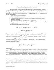
Implementation Example: Calculating Pi 

Generate random points inside a square 

Identify fraction (f) that fall inside a circle with radius equal 

to box width 

x 2 + y 2 < r 

Area of quarter of circle (A) = pi*r 2 / 4 

Area of square (B) = r 2 

A/B = f = pi/4 

pi = 4f

Calculating pi with threads 

from threading import Thread 

from Queue import Queue, Empty 

import random 

def calcInside(nsamples,rank): 

global inside #we need something everyone can share 

random.seed(rank) 

for i in range(nsamples): 

x = random.random(); 

y = random.random(); 

if (x*x)+(y*y)

Subprocess 

The subprocess module allows the Python interpreter to 

spawn and control processes. It is unaffected by the GIL. Using 

the subprocess.Popen() call, one may start any process 

you'd like. 

>>> pi=subprocess.Popen('python -c "import math; print 

math.pi"',shell=True,stdout=subprocess.PIPE) 

>>> pi.stdout.read() 

'3.14159265359\n' 

>>> pi.pid 

1797 

>>> me.wait() 

0 

It goes without saying, there's better ways to do 

subprocesses...

Multiprocessing 

Added in Python 2.6 

Faster than threads as the GIL is sidestepped 

uses subprocesses 

both local and remote subprocesses are supported 

shared memory between subprocesses is risky 

no coherent types 

Array and Value are built in 

others via multiprocessing.sharedctypes 

IPC via pipes and queues 

pipes are not entirely safe 

synchronization via locks 

Manager allows for safe distributed sharing, but it's slower 

than shared memory

Calculating pi with multiprocessing 

import multiprocessing as mp 

import numpy as np 

import random 

processes = mp.cpu_count() 

nsamples = 120000/processes 

def calcInside(rank): 

inside = 0 





if (x*x)+(y*y)

pi with multiprocessing, optimized 

import multiprocessing as mp 


processes = mp.cpu_count() 

nsamples = 120000/processes 

def calcInsideNumPy(rank): 

np.random.seed(rank) 

xy = np.random.random((nsamples,2))**2 # "vectorized" sample gen 

return 4.0*np.sum(np.sum(xy,1)

mpi4py 

wraps your native mpi 

prefers MPI2, but can work with MPI1 

works best with NumPy data types, but can pass around 

any serializable object 

provides all MPI2 features 

well maintained 

distributed with Enthought's SciPy 

requires NumPy 

portable and scalable 

http://mpi4py.scipy.org/

How mpi4py works... 

mpi4py jobs must be launched with mpirun 

each rank launches its own independent python interpreter 

each interpreter only has access to files and libraries 

available locally to it, unless distributed to the ranks 

communication is handled by your MPI layer 

any function outside of an if block specifying a rank is 

assumed to be global 

any limitations of your local MPI are present in mpi4py

from mpi4py import MPI 


import random 

comm = MPI.COMM_WORLD 

rank = comm.Get_rank() 

mpisize = comm.Get_size() 

nsamples = 120000/mpisize 

inside = 0 





if (x*x)+(y*y)

Performance 

Best practices with pure Python & NumPy 

Optimization where needed (we'll talk about this in GPAW) 

profiling 

inlining 

Other avenues

Python Best Practices for Performance 

If at all possible... 

Don't reinvent the wheel. 

someone has probably already done a better job than 

your first (and probably second) attempt 

Build your own modules against optimized libraries 

ESSL, ATLAS, FFTW, PyCUDA, PyOpenCL 

Use NumPy data types instead of Python ones 

Use NumPy functions instead of Python ones 

"vectorize" operations on >1D data types. 

avoid for loops, use single-shot operations 

Pre-allocate arrays instead of repeated concatenation 

use numpy.zeros, numpy.empty, etc..

Real-World Examples and Techniques: 

GPAW

Outline 

a massively parallel Python-C code for KS-DFT 

Introduction 

NumPy 

Memory 

FLOPs 

Parallel-Python Interpreter and Debugging 

Profiling mixed Python-C code 

Python Interface BLACS and ScaLAPACK 

Concluding remarks

Overview 

GPAW is an implementation of the projector augmented 

wave method (PAW) method for Kohn-Sham (KS) - 

Density Functional Theory (DFT) 

Mean-field approach to Schrodinger equation 

Uniform real-space grid, multiple levels of parallelization 

Non-linear sparse eigenvalue problem 

10^6 grid points, 10^3 eigenvalues 

Solved self-consistently using RMM-DIIS 

Nobel prize in Chemistry to Walter Kohn (1998) for (KS)-DFT 

Ab initio atomistic simulation for predicting material 

properties 

Massively parallel and written in Python-C using the 

NumPy library.

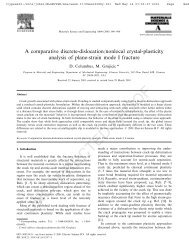
GPAW Strong-scaling Results

GPAW code structure 

Not simply a Python wrapper on legacy Fortran/C code 

Python for coding the high-level algorithm, lots of OO 

C for coding numerical intense operations, built on NumPy 

Use BLAS and LAPACK whenever possible 

Here is some pseudo code for iterative eigensolver: 

for i in xrange(max SCF): 

for n in xrange(number of bands): 

R_ng = apply(H_gg,Psi_ng) % Compute residuals 

rk(1.0, R_ng, 0.0, H_mn) % construct Hamiltonian 

KS-DFT algorithms are well-known and computationally 

intensive parts are known a priori.

KS-DFT is a complex algorithm!

Source Code History 

Mostly Python-code, 10% C-code. 

90% of wall-clock time spend in C, BLAS, and LAPACK.

Performance Mantra 

People are able to code complex algorithms in much less time 

by using a high-level language like Python (e.g., also 

C++). There can be a performance penalty in the most pure 

sense of the term. 

"The best performance improvement is the transition from the 

nonworking to the working state." 

--John Ousterhout 

"Premature optimization is the root of all evil." 

--Donald Knuth 

"You can always optimize it later." 

-- Unknown

NumPy - Memory 

Q: Where is all my memory going? 

A: It disappears a little bit at a time. 

BlueGene/P has 512 MB per core. 

Compute note kernel is another 34 MB. 

NumPy library is ~ 38 MB. 

Python Interpreter 12 MB. 

Can't always get the last 50 MB, NumPy to blame? 

Try this simple test: 


A = np.zero((N,N),dtype=float) 

Beware of temporary matrices, they are sometimes not 

obvious 

D = np.dot(A,np.dot(B,C))

NumPy - Memory 

How big is your binary? Find out using 'size ' 

GPAW is 70 MB without all the dynamic libraries. 

Only 325 MB of memory left on BG/P per core for 

calculation! 

FLOPS are cheap, memory and bandwidth are expensive! 

Future supercomputers will have low memory per core.

NumPy - FLOPS 

Optimized BLAS available via NumPy via np.dot. Handles 

general inner product of multi-dimensional arrays. 

Very difficult to cross-compile on BG/P. Blame disutils! 

core/_dotblas.so is a sign of optimized NumPy dot 

Python wrapper overhead is negligible 

For matrix * vector products, NumPy dot can yield better 

performance than direct call to GEMV! 

Fused floating-point multiply-add instructions are not 

created for AXPY type operation in pure Python. Not 

available in NumPy either. 

for i in xrange(N): 

Y[i] += alpha*X[i] 

C[i] += A[i]*B[i]

NumPy - FLOPS 

WARNING: If you make heavy, use of BLAS & LAPACK type 

operations. 

Plan on investing a significant amount of time working to 

cross-compile optimized NumPy. 

Safest thing is to write your own C-wrappers. 

If all your NumPy arrays are < 2-dimensional, Python 

wrappers will be simple. 

Wrappers for multi-dimensional arrays can be challenging: 

SCAL, AXPY is simple 

GEMV more difficulty 

GEMM non-trivial 

Remember C & NumPy arrays are row-ordered, Fortran 

arrays are column-ordered!

Python BLAS Interface 

void dscal_(int*n, double* alpha, double* x, int* incx); % C prototype for Fortran 

void zscal_(int*n, void* alpha, void* x, int* incx); % C prototype for Fortran 

#define DOUBLEP(a) ((double*)((a)->data)) % Casting for NumPy data struc. 

#define COMPLEXP(a) ((double_complex*)((a)->data)) % Casting for NumPy data struc. 

PyObject* scal(PyObject *self, PyObject *args) 

{ 

Py_complex alpha; 

PyArrayObject* x; 

if (!PyArg_ParseTuple(args, "DO", &alpha, &x)) 

return NULL; 

int n = x->dimensions[0]; 

for (int d = 1; d < x->nd; d++) % NumPy arrays can be multi-dimensional! 

n *= x->dimensions[d]; 

int incx = 1; 

} 

if (x->descr->type_num == PyArray_DOUBLE) 

dscal_(&n, &(alpha.real), DOUBLEP(x), &incx); 

else 

zscal_(&n, &alpha, (void*)COMPLEXP(x), &incx); 

Py_RETURN_NONE;

Profiling Mixed Python-C code 

Number of profiling tools available: 

gprof, CrayPAT, import profile 

gprof, CrayPAT - C, Fortran 

import profile - Python 

TAU, http://www.cs.uoregon.edu/research/tau/home.php 

Exclusive time for C, Python, MPI are reported 

Communication matrix available 

Interfaces with PAPI for performance counters 

Manual and automatic instrumentation available 

Installation is doable, but can be challenging 

Finding performance bottlenecks is critical to scalability on 

HPC platforms

Parallel Python Interpreter and 

Debugging


Debugging 

MPI-enabled "embedded" Python Interpreter: 

int main(int argc, char **argv) 

{ 

int status; 

MPI_Init(&argc, &argv); % backwards compatible with MPI-1 

Py_Initialize(); % needed because of call in next line 

PyObect* m = Py_InitModule3("_gpaw", functions, 

"C-extension for GPAW\n\n... 

\n"); 

import_array1(-1); % needed for NumPy C-API 

MPI_Barrier(MPI_COMM_WORLD); % sync up 

status = Py_Main(argc, argv); % call to Python Interpreter 

MPI_Finalize(); 

return status; 

}


Debugging 

Errors in Python modules are OK, core dumps in C extensions 

are problematic: 

Python call stack is hidden; this is due to Python's 

interpreted nature. 

Totalview won't help, sorry.


Flat profile shows time spent in Python, C, and MPI simultaneously:


Measure heap memory on subroutine entry/exit:

Python Interface to BLACS and ScaLAPACK 

Parallel dense linear algebra needed for KS-DFT. As the matrix 

size N grows, this operation cannot be performed in serial. 

(approx. cross over point) 

symmetric diagonalize (N > 1000) 

symmetric general diagonalize (N > 1000) 

inverse Cholesky (N > 4000) 

There is no parallel dense linear algebra in NumPy, there are 

some options: 

PyACTS, based on Numeric 

GAiN, Global Arrays based on NumPy (very new) 

Write your own Python interface to ScaLAPACK.


Mostly non-Python related challenges: 

Good ScaLAPACK examples are few and far apart. 

DFT leads to wieldy use of ScaLAPACK 

H_mn is on a small subset of MPI_COMM_WORLD 

ScaLAPACK does not create a distribute object for you. 

Array must be created in a distributed manner 

ScaLAPACK allows you to manipulate them via 

descriptors 

Array must be compatible with their native 2D-block 

cyclic layout 

What language was used to write ScaLAPACK and 

BLACS? 

C and Fortran 

Distributed arrays assumed to be Fortran-ordered.


MPI_COMM_WORLD on a 512-node on 8x8x8 BG/P. 

2048 cores!


Physical 1D layout (left) of H_mn, need to redistribute to 2D 

block-cyclic layout (right) for use with ScaLAPACK.


BLACS: 

Cblacs_gridexit 

Cblacs_gridinfo 

Cblacs_gridinit 

Cblacs_pinfo 

Csys2blacs_handle 

Python: 

blacs_create 

blacs_destroy 

blacs_redist 

ScaLAPACK: 

numroc 

Cpdgem2d 

Cpzgemm2d 

Cpdgemr2do 

Cpzgemr2do


Important to understand notion of array descriptor: 

Distinguish between global and local array. Create local 

array in parallel. 

int desc[9]; 

desc[0] = BLOCK_CYCLIC_2D; % MACRO = 1 

desc[1] = ConTxt; % must equal -1 if inactive 

desc[2] = m; % number of rows in global array 

desc[3] = n; % number of columns in global array 

desc[4] = mb; % row blocksize 

desc[5] = nb; % column blocksize 

desc[6] = irsrc; % starting row 

desc[7] = icsrc; % starting column 

desc[8] = MAX(0, lld); % leading dimension of local array


Descriptor only missing ConTxt and LLD, all else from inputs! 

Pyobject* blacs_create(PyObject *self, PyObject *args) 

{ 

if (!PyArg_ParseTuple(args, "Oiiiiii|c", &comm_obj, &m, &n, 

&nprow, 

&npco 

l, &mb, &nb, &order)) 

return NULL; 

if (comm_obj == Py_None) % checks for MPI_COMM_NULL 

create inactive descriptor 

else { 

MPI_Comm comm = ((MPIObject*)comm_obj->comm; 

ConTxt = Csys2blacs_handle(comm); % ConTxt out of Comm 

Cblacs_gridinit(&ConTxt, &order, nprow, npcol); 

Cblacs_gridinfo(ConTxt, &nprow, &npcol, &myrow, &mycol); 

LLD = numroc(&m, &mb, &mrow, &rsrc, &nprow); 

create active descriptor 

} 

return desc as PyObject 

}

Python Interface in BLACS and ScaLAPACK 

PyObject* scalapack_redist(PyObject *self, PyObject *args) 

{ 

PyArrayObject* a_obj; % source matrix 

PyArrayObject* b_obj; % destination matrix 

PyArrayObject* adesc; % source descriptor 

PyArrayObject* bdesc; % destination descriptor 

PyObject* comm_obj = Py_None; % intermediate communicator 

if (!PyArg_ParseTuple(args, "OOOi|Oii", &a_obj, &adesc, 

&bdesc, &isreal, &comm_obj, &m, &n)) 

return NULL; 

% Get info about source (a_ConTxt) and destination (b_ConTxt) grid; 

Cblacs_gridinfo_(a_ConTxt, &a_nprow, &a_npcol,&a_myrow, 

&a_mycol); 

Cblacs_gridinfo_(b_ConTxt, &b_nprow, &b_npcol,&b_myrow, 

&b_mycol); 

% Size of local destination array 

int b_locM = numroc_(&b_m, &b_mb, &b_myrow, &b_rsrc, &b_nprow); 

int b_locN = numroc_(&b_n, &b_nb, &b_mycol, &b_csrc, &b_npcol);


% Size of local destination array 

int b_locM = numroc_(&b_m, &b_mb, &b_myrow, &b_rsrc, &b_nprow); int 

b_locN = numroc_(&b_n, &b_nb, &b_mycol, &b_csrc, &b_npcol); 

% Create Fortran-ordered NumPy array 

npy_intp b_dims[2] = {b_locM, b_locN); 

if (isreal) 

b_obj = (PyArrayObject*)PyArray_EMPTY(2, b_dims, NPY_DOUBLE, 

NPY_F_CONTIGUOUS); 

else 

b_obj = (PyArrayObject*)PyArray_EMPTY(2, b_dims, 

NPY_DOUBLE, NPY_F_CONTIGUOUS);


if (comm_obj = Py_None) % intermediate communicator is world 

{ 

if(isreal) 

Cpdgemr2do_(m, n, DOUBLEP(a_obj), one, one, INTP(adesc), 

DOUBLEP(b_obj), one, one, INTP 

(bdesc)); 

else 

Cpzgem2rdo_(m, n, (void*)COMPLEXP(a_obj), one, one, 

INTP(adesc), (void*)COMPLEXP(b_obj), 

one, one, 

INTP(bdesc)); 

} 

else % intermediate communicator is user-defined 

 

if(isreal) 

Cpdgemr2d(.....); 

else 

Cpzgemr2d(......); 

}


Source blacs grid (blue) and destination blacs grid (red). 

Intermediate blacs grid for scalapack_redist: 

Must call Cp[d/z]gemr2d[o] 

Must encompass both source and destination 

For multiple concurrent redist operations, intermediate 

cannot overlap.


% Note that we choose to return Py_None, instead of empty array. 

if ((b_locM == 0) | (b_locN == 0)) 

{ 

Py_DECREF(b_obj); 

Py_RETURN_NONE; 

} 

PyObject* value = PyBuildValue("O",b_obj); 

Py_DECREF(b_obj); 

return value; 

} % end of scalapack_redist 

More information at: 

https://trac.fysik.dtu.dk/projects/gpaw/browser/trunk/c/blacs.c

The Bad & Ugly: 

NumPy cross-compile. 

C Python extensions require 

learning NumPy & C API. 

Debugging C extensions can be 

difficult. 

Performance analysis will 

always be needed. 

OpenMP-like threading not 

available due to GIL. 

Python will need to support 

GPU acceleration in the future. 

Summary 

The Good: 

GPAW has an extraordinary amount 

of functionality and scalibity. A lot of 

features make coding complex 

algorithms easy: 

OOP 

weakly-typed data structures 

Interface with many things other 

languages: C, C++, Fortran, etc.

Success Story 

GPAW will allow you to run multiple concurrent DFT calculations with 

a single executable. 

High-throughput computing (HTC) for catalytic materials screening. 

Perform compositional sweeps trivially. 

Manage the dispatch of many tasks without 3rd party software 

Suppose 512-node partition, 2048 cores 

Each DFT calculation requires 128 cores, no guarantee that 

they all finish at the same time 

Set-up for N >> 2048/128 calculations. As soon as one DFT 

calculations finish, start another one until the job runs out of 

wall-clock time.

Python for plotting and visualization 

Overview of matplotlib 

Example of MC analysis tool written in Python 

Looking at data sharing on the web

From a Scientific Library 

To a Scientific Application 

Massimo Di Pierro

From Lib to App 

(overview) 

Numerical Algorithms

Storage 


(overview) 

Numerical Algorithms 

Store and retrieve information in a relational database


(overview) 

Storage Numerical Algorithms 

Interface 

Plotting 

Store and retrieve information in a relational database 

Provide a user interface 

input forms with input validation 

represent data (html, xml, csv, json, xls, pdf, rss) 

represent data graphically


(overview) 

Storage Numerical Algorithms 

Interface 

Plotting 

Store and retrieve information in a relational database 

Provide a user interface 

input forms with input validation 

represent data (html, xml, csv, json, xls, pdf, rss) 

represent data graphically 

Communicate with users over the internet 

provide user authentication/authorization/access control 

provide persistence (cookies, sessions, cache) 

log activity and errors 

protect security of data 

internet 

user 

user 

user

Ruby on Rails 

Django 

TurboGears 

Pylons 

... 

web2py 

How? Use a framework! 

gnuplot.py 

r.py 

Chaco 

Dislin 

... 

matplotlib

Why? 

web2py is really easy to use 

web2py is really powerful and does a lot 

for you 

web2py is really fast and scalable for 

production jobs 

I made web2py so I know it best 

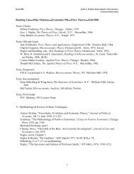
matplotlib is the best library for plotting I 

have ever seen (not just in Python)

matplotlib gallery

web2py and MVC 

code project

application1 

application 

2 

application 

3 


code project

application 

1 

application=” 

dna” 

application 

3 


Models Controllers Views 

code project 

Data 

representation 

Logic/Workflow 

Data 

presentation

application 

1 

application=” 

dna” 

application 

3 


Models Controllers Views 

code project 

db.define_table( 

‘dna’, 

Field(‘sequence’)) 

Data 

representation 

def upload_dna(): 

return dict(form= 

crud.create(db.dna)) 

Logic/Workflow 

 

Upload DNA Seq. 

 

{{=form}} 

Data 

presentation 

Minimal 

Complete 

Application


 

{{=form}} 

web2py and Dispatching

web2py and Dispatching 

hostnam 

e


app name


controller


action 

name


 

{{=form}} 

web2py and Views


 

{{=form}} 

web2py and Views 

{{=form}}

web2py and Authentication 

authenticatio 

n

web2py and AppAdmin 

database interface

web2py web based IDE 

web based IDE

Goal 

to build a web based application 

that stores DNA sequences 

allows upload of DNA sequences 

allows analysis of DNA sequences 

(reverse, count, align, etc.) 

allows plotting of results

Before we start 

download web2py from web2py.com 

unzip web2py and click on the executable 

when it asks for a password choose one 

visit http://127.0.0.1:8000/admin and login 

create a new “dna” application by: 

type “dna” in the apposite box and press [submit]

import math, random, uuid, re 

db.define_table('dna', 

Field('name'), 

Field('sequence','text')) 

Define model 

in models/db_dna.py 

def random_gene(n): 

return ''.join(['ATGC'[int(n+10*math.sin(n*k)) % 4] \ 

for k in range(10+n)])+'UAA' 

def random_dna(): 

return ''.join([random_gene(random.randint(0,10)) \ 

for k in range(50)]) 

if not db(db.dna.id>0).count(): 

for k in range(100): 

db.dna.insert(name=uuid.uuid4(),sequence=random_dna())

Define some algorithms 

def find_gene_size(a): 

r=re.compile('(UAA|UAG|UGA)(?P.*?)(UAA|UAG|UGA)') 

return [(g.start(),len(g.group('gene'))) \ 

for g in r.finditer(a)] 

def needleman_wunsch(a,b,p=0.97): 

"""Needleman-Wunsch and Smith-Waterman""" 

z=[] 

for i,r in enumerate(a): 

z.append([]) 

for j,c in enumerate(b): 

if r==c: 

z[-1].append(z[i-1][j-1]+1 if i*j>0 else 1) 

else: 

z[-1].append(p*max(z[i-1][j] if i>0 else 0, 

z[i][j-1] if j>0 else 0)) 

return z

in models/matplotlib_helpers.py 

import random, cStringIO 

from matplotlib.backends.backend_agg import FigureCanvasAgg as FigureCanvas 

from matplotlib.figure import Figure 

def plot(title='title',xlab='x',ylab='y',data={}): 

fig=Figure() 

fig.set_facecolor('white') 

ax=fig.add_subplot(111) 

if title: ax.set_title(title) 

if xlab: ax.set_xlabel(xlab) 

if ylab: ax.set_ylabel(ylab) 

legend=[] 

keys=sorted(data) 

for key in keys: 

stream = data[key] 

(x,y)=([],[]) 

for point in stream: 

x.append(point[0]) 

y.append(point[1]) 

ell=ax.hist(y,20) 

canvas=FigureCanvas(fig) 

response.headers['Content-Type']='image/png' 

stream=cStringIO.StringIO() 

canvas.print_png(stream) 

return stream.getvalue()

Define actions 

in controllers/default.py 

def index(): 

rows=db(db.dna.id).select(db.dna.id,db.dna.name) 

return dict(rows=rows) 

@auth.requires_login() 

def gene_size(): 

dna = db.dna[request.args(0)] or \ 

redirect(URL(r=request,f='index')) 

lengths = find_gene_size(dna.sequence) 

return hist(data={'Lengths':lengths})

{{extend 'layout.html'}} 

Define Views 

in views/default/index.html 

compare 

 

{{for row in rows:}} 

{{=row.name}} 

[gene sizes] 

 

{{pass}} 

Try it

in models/matplotlib_helpers.py 

def pcolor2d(title='title',xlab='x',ylab='y', 

z=[[1,2,3,4],[2,3,4,5],[3,4,5,6],[4,5,6,7]]): 

fig=Figure() 

fig.set_facecolor('white') 

ax=fig.add_subplot(111) 

if title: ax.set_title(title) 

if xlab: ax.set_xlabel(xlab) 

if ylab: ax.set_ylabel(ylab) 

image=ax.imshow(z) 

image.set_interpolation('bilinear') 

canvas=FigureCanvas(fig) 

response.headers['Content-Type']='image/png' 

stream=cStringIO.StringIO() 

canvas.print_png(stream) 

return stream.getvalue()

Define Actions 

in controllers/default.py 

def needleman_wunsch_plot(): 

dna1 = db.dna[request.vars.sequence1] 

dna2 = db.dna[request.vars.sequence2] 

z = needleman_wunsch(dna1.sequence,dna2.sequence) 

return pcolor2d(z=z) 

def compare(): 

form = SQLFORM.factory( 

Field('sequence1',db.dna, 

requires=IS_IN_DB(db,'dna.id','%(name)s')), 

Field('sequence2',db.dna, 

requires=IS_IN_DB(db,'dna.id','%(name)s'))) 

if form.accepts(request.vars): 

image=URL(r=request,f='needleman_wunsch_plot', 

vars=form.vars) 

else: 

image=None 

return dict(form=form, image=image)

{{extend 'layout.html'}} 

{{=form}} 

Define Views 

in views/default/compare.html 

{{if image:}} 

Sequence1 = {{=db.dna[request.vars.sequence1].name}} 

Sequence2 = {{=db.dna[request.vars.sequence2].name}} 

 

{{pass}}

Try it

Resources 

Python 

http://www.python.org/ 

all the current documentation, software, tutorials, news, and pointers to advice 

you'll ever need 

GPAW 

https://wiki.fysik.dtu.dk/gpaw/ 

GPAW documentation and code 

SciPy and NumPy 

http://numpy.scipy.org/ 

The official NumPy website 

http://conference.scipy.org/ 

The annual SciPy conference 

http://www.enthought.com/ 

Enthought, Inc. the commercial sponsors of SciPy, NumPy, Chaco, EPD and 

more 

Matplotlib 

http://matplotlib.sourceforge.net/ 

best 2D package on the planet 

mpi4py 

http://mpi4py.scipy.org/

Yet More Resources 

Tau 

http://www.cs.uoregon.edu/research/tau/home.php 

official open source site 

http://www.paratools.com/index.php 

commercial tools and support for Tau 

web2py 

http://www.web2py.com/ 

web framework used in this tutorial

Hey! There's a Python BOF 

Python for High Performance and Scientific Computing 

Primary Session Leader: 

Andreas Schreiber (German Aerospace Center) 

Secondary Session Leaders: 

William R. Scullin (Argonne National Laboratory) Steven 

Brandt (Louisiana State University) James B. Snyder (Northwestern 

University) Nichols A. Romero (Argonne National Laboratory) 

Birds-of-a-Feather Session 

Wednesday, 05:30PM - 07:00PM Room A103-104 

Abstract: 

The Python for High Performance and Scientific Computing BOF is intended to 

provide current and potential Python users and tool providers in the high 

performance and scientific computing communities a forum to talk about their 

current projects; ask questions of experts; explore methodologies; delve into 

issues with the language, modules, tools, and libraries; build community; and 

discuss the path forward.

Let's review!

Questions?

This work is supported in part by the 

resources of the Argonne Leadership 

Computing Facility at Argonne National 

Laboratory, which is supported by the 

Office of Science of the U.S. Department 

of Energy under contract DE-AC02- 

06CH11357. 

Extended thanks to 

Northwestern University 

De Paul University 

the families of the presenters 

Sameer Shende, ParaTools, Inc. 

Enthought, Inc. for their continued 

support and sponsorship of SciPy 

and NumPy 

Lisandro Dalcin for his work on 

mpi4py and tolerating a lot of 

questions 

Acknowledgments 

the members of the Chicago Python 

User's Group (ChiPy) for allowing us 

to ramble on about science and HPC 

the Python community for their 

feedback and support 

CCT at LSU 

numerous others at HPC centers 

nationwide

Tutorial slides (PDF) - Clemson University

Create successful ePaper yourself

Delete template?

Save as template?