A VISUAL INFORMATION FIDELITY APPROACH TO VIDEO ...
A VISUAL INFORMATION FIDELITY APPROACH TO VIDEO ...
A VISUAL INFORMATION FIDELITY APPROACH TO VIDEO ...
You also want an ePaper? Increase the reach of your titles
YUMPU automatically turns print PDFs into web optimized ePapers that Google loves.
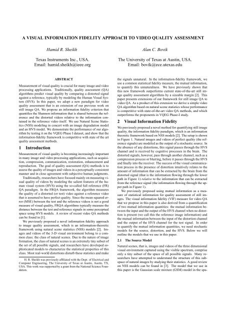
A <strong>VISUAL</strong> <strong>INFORMATION</strong> <strong>FIDELITY</strong> <strong>APPROACH</strong> <strong>TO</strong> <strong>VIDEO</strong> QUALITY ASSESSMENT<br />
Hamid R. Sheikh<br />
Texas Instruments Inc., USA.<br />
Email: hamid.sheikh@ieee.org<br />
ABSTRACT<br />
Measurement of visual quality is crucial for many image and video<br />
processing applications. Traditionally, quality assessment (QA)<br />
algorithms predict visual quality by comparing a distorted signal<br />
against a reference, typically by modeling the Human Visual System<br />
(HVS). In this paper, we adopt a new paradigm for video<br />
quality assessment that is an extension of our previous work on<br />
still image QA. We propose an information fidelity criterion that<br />
quantifies the Shannon information that is shared between the reference<br />
and the distorted videos relative to the information contained<br />
in the reference video itself. We use Natural Scene Statistics<br />
(NSS) modeling in concert with an image degradation model<br />
and an HVS model. We demonstrate the performance of our algorithm<br />
by testing it on the VQEG Phase I dataset, and show that the<br />
information-fidelity framework is competitive with state of the art<br />
quality assessment methods.<br />
1 Introduction<br />
Measurement of visual quality is becoming increasingly important<br />
in many image and video processing applications, such as acquisition,<br />
compression, communication, restoration, enhancement and<br />
reproduction. The goal of quality assessment (QA) methods is to<br />
assess the quality of images and videos in a perceptually consistent<br />
manner and in close agreement with subjective human judgments.<br />
Traditionally, researchers have focused mainly on measuring visual<br />
quality of videos by modeling the salient features of the human<br />
visual system (HVS) using the so-called full reference (FR)<br />
QA paradigm. In the FRQA framework, the algorithm measures<br />
the quality of a distorted (or test) video against a reference video<br />
that is assumed to have perfect quality. Since the mean squared error<br />
(MSE) between the test and the reference videos is not a good<br />
measure of visual quality, FRQA algorithms typically measure the<br />
distance between the test and reference signals in some perceptual<br />
space using HVS models. A review of recent video QA methods<br />
can be found in [1].<br />
We previously proposed a novel information fidelity approach<br />
to image quality assessment, which is an information-theoretic<br />
framework using natural scene statistics (NSS) models [2]. Images<br />
and videos of the 3-D visual environment belong to a common<br />
class: the class of natural scenes. Due to the nature of image<br />
formation, the class of natural scenes is an extremely tiny subset of<br />
the set of all possible signals, and researchers have developed sophisticated<br />
models to characterize the statistical properties of this<br />
class. Most real-world distortions disturb these statistics and make<br />
H. R. Sheikh was previously affiliated with the Dept. of Electrical and<br />
Computer Engineering, The University of Texas at Austin, Austin, TX,<br />
USA. This work was supported by a grant from the National Science Foundation.<br />
Alan C. Bovik<br />
The University of Texas at Austin, USA.<br />
Email: bovik@ece.utexas.edu<br />
the signals unnatural. In the information-fidelity framework, we<br />
use a common statistical fidelity measure, the mutual information,<br />
to quantify this unnaturalness. We have previously shown that<br />
this new framework outperforms current state-of-the-art still image<br />
quality assessment algorithms by a sizeable margin [2]. This<br />
paper presents extensions of our framework for still image QA to<br />
video QA. As a product of this extension we derive a simple video<br />
QA algorithm based on natural scene statistics whose performance<br />
is competitive with state-of-the-art video QA methods, and which<br />
outperforms the proponents in VQEG Phase-I study.<br />
2 Visual Information Fidelity<br />
We previously proposed a novel method for quantifying still image<br />
quality, the information fidelity paradigm, which is an information<br />
theoretic framework based on NSS models [2]. The setup is shown<br />
in Figure 1. Natural images and videos of perfect quality (the reference<br />
signals) are modeled as the output of a stochastic source. In<br />
the absence of any distortions, this signal passes through the HVS<br />
channel and is received by cognitive processes in the brain. The<br />
distorted signals, however, pass through another channel, such as a<br />
compression process or blurring, before it passes through the HVS<br />
and finally into the receiver. The success of the visual communication<br />
process in the presence of distortion intuitively relates to the<br />
amount of information that can be extracted by the brain from the<br />
distorted signal (that is the information flowing through the lower<br />
path in Figure 1) relative to the information that can be extracted<br />
from the reference signal (the information flowing through the upper<br />
path in Figure 1).<br />
We previously proposed using mutual information as a measure<br />
of statistical information for quality assessment of still images.<br />
The visual information fidelity (VIF) measure for video QA<br />
that we propose in this paper is also derived from a quantification<br />
of two mutual information quantities: the mutual information between<br />
the input and the output of the HVS channel when no distortion<br />
is present (we call this the reference image information) and<br />
the mutual information between the input of the distortion channel<br />
and the output of the HVS channel for the test signal. In order<br />
to quantify the mutual information quantities, we need stochastic<br />
models for the source, distortion, and the HVS. Below we will<br />
outline the models that we use in this paper.<br />
2.1 The Source Model<br />
Natural scenes, that is, images and videos of the three dimensional<br />
visual environment captured using the visible spectrum, comprise<br />
only a tiny subset of the space of all possible signals. Many researchers<br />
have attempted to understand the structure of this subspace<br />
of natural images by studying their statistics. A good review<br />
on NSS models can be found in [3]. The model that we use in<br />
this paper is the Gaussian scale mixture (GSM) model in the spa-
Natural scene<br />
source<br />
Reference<br />
HVS<br />
Channel Test<br />
HVS<br />
C (Distortion) D F<br />
E<br />
Receiver<br />
Receiver<br />
Fig. 1. Mutual information between C and E quantifies the information<br />
that the brain could ideally extract from the reference<br />
signal, whereas the mutual information between C and F quantifies<br />
the corresponding information that could be extracted from the<br />
distorted signal.<br />
tiotemporal derivative (horizontal, vertical, and temporal discretederivatives<br />
[4]) domain. We have previously successfully used the<br />
GSM model in the wavelet domain for image quality assessment<br />
using a similar information fidelity setup [2]. In order to use this<br />
model for video, we first need to motivate the suitability of this<br />
model for videos.<br />
2.1.1 Image Formation<br />
Researchers have argued that the peculiar statistics of natural images<br />
come from the physics of image formation [5, 6]. The laws<br />
that govern the formation of light stimulus that emanates from the<br />
environment dictate the statistics of the signal. Researchers have<br />
identified occlusion as the image formation rule that leads to many<br />
of the observed statistics of natural images. That is, images are<br />
formed when objects occlude each other, generally blocking the<br />
light signal coming from objects ‘behind them’. This leads to images<br />
that contain smooth or textured regions separated by strong<br />
edges at object boundaries. Thus, when such an image is filtered<br />
through a zero-mean kernel (a high-pass or a band-pass filter), the<br />
resulting coefficients tend to have a histogram that has a sharp peak<br />
at zero and tails that fall off slowly. The smooth textures give rise<br />
to generally low magnitude coefficients (and hence the sharp peak<br />
at zero in the histogram), while the strong edges yield high magnitude<br />
coefficients (heavy tails) typically observed in natural images.<br />
2.1.2 Occlusion in Natural Videos<br />
It is obvious that occlusion continues to operate even for natural<br />
videos. Thus, applying spatial zero-mean kernels would still<br />
give the characteristic histograms. Moreover, it is easy to explain<br />
why such kernels would give similar histograms even when applied<br />
along the temporal domain. Consider two one-dimensional<br />
objects in Figure 2 that are being observed through a camera in<br />
a two dimensional world. When object A moves and occludes<br />
object B, one could see occlusion of B by A in a spatiotemporal<br />
plane much like the occlusion of objects in still images. The spatiotemporal<br />
plane consists of generally smooth ‘objects’ separated<br />
by sharp edges that result from ‘occlusion’ of spatiotemporal objects,<br />
and hence the temporal channel should exhibit similar statistical<br />
properties as the spatial channels. The argument could easily<br />
be extended to a three dimensional case.<br />
Indeed, this hypothesis holds when one observes the histograms<br />
of temporally filtered natural videos. Figure 3 shows the histogram<br />
of the temporal derivative of ‘Mobile and Calendar’. As expected,<br />
the histogram has a sharp peak at zero and heavy tails. Moreover,<br />
the temporal coefficients also exhibit linear and nonlinear dependencies<br />
similar to those observed in spatial coefficients of images<br />
[7]. This is illustrated in Figure 4, which shows the joint histogram<br />
of the logarithm of the magnitude of two temporally adjacent coef-<br />
B<br />
Camera<br />
A<br />
Time<br />
Space<br />
Fig. 2. Spatiotemporal representation of motion. Object A moves<br />
and occludes B, which is stationary. Occlusion manifests in the<br />
spatiotemporal domain as spatiotemporal objects ‘occluding’ each<br />
other, similar to spatial-only images.<br />
Count<br />
10 6<br />
10 5<br />
10 4<br />
10 3<br />
10 2<br />
10 1<br />
10<br />
−50 0 50<br />
0<br />
Coefficient<br />
Fig. 3. Histogram of coefficients of a bandpass channel of ‘Mobile<br />
and Calendar’ video shows a sharp peak and heavy tails.<br />
ficients C1 and C2 in the temporal-derivative channel 1 . The linear<br />
dependency between the logarithm of the coefficient magnitudes<br />
demonstrates a multiplicative dependency between the coefficient<br />
magnitudes, which can be modeled well though a GSM model [7].<br />
Moreover, divisively normalizing the coefficients by estimates of<br />
local standard deviation removes this dependency, as shown in Figure<br />
4. We therefore conclude that the spatial and temporal channels<br />
of natural videos (such as those resulting from discrete derivatives<br />
for optical flow estimation or other 3D transformations such as<br />
wavelet decompositions) could be modeled well by GSMs.<br />
2.1.3 Representation of Motion<br />
The use of intensity derivatives for optical flow estimation is<br />
widely known in the image processing community. Researchers<br />
have also explored possible connections between motion representation<br />
in HVS and spatiotemporal derivatives and their approximation<br />
using bandpass kernels [8]. In the information-fidelity framework,<br />
although we do not deal directly with motion representation,<br />
derivative information does form a bound on motion information.<br />
Any loss in derivative information (which we shall quantify later<br />
in this paper) would necessarily cause a loss in motion information<br />
in the signal.<br />
2.1.4 Gaussian Scale Mixture Model<br />
A GSM is a random field (RF) that can be expressed as a product<br />
of two independent RFs [7] . That is, a GSM C = { −→ C i : i ∈<br />
I}, where I denotes the set of spatial indices for the RF, can be<br />
1 Linear dependency between C1 and C2 was removed before plotting<br />
the histograms to highlight the nonlinear dependency.
Log 10 (Abs(C 2 ))<br />
Log 10 (Abs(C 2 /S 2 ))<br />
3<br />
2<br />
1<br />
0<br />
−1<br />
−2<br />
−3<br />
−3 −2 −1 0<br />
Log (Abs(C ))<br />
10 1<br />
1 2 3<br />
3<br />
2<br />
1<br />
0<br />
−1<br />
−2<br />
−3<br />
−3 −2 −1 0<br />
Log (Abs(C /S ))<br />
10 1 1<br />
1 2 3<br />
Fig. 4. Joint histograms of temporally adjacent coefficients before<br />
and after normalization. See text.<br />
expressed as:<br />
C = S · U = {Si · −→ U i : i ∈ I} (1)<br />
where S = {Si : i ∈ I} is an RF of positive scalars and<br />
U = { −→ U i : i ∈ I} is a Gaussian vector RF with mean zero and<br />
covariance CU . −→ C i and −→ U i are M dimensional vectors. In this<br />
paper we model each channel (output of a spatiotemporal kernel)<br />
as a GSM. We partition a channel into non-overlapping spatiotemporal<br />
blocks, and model each block as the vector −→ C i.<br />
We model each channel with a separate GSM. However, we will<br />
only deal with one channel here and later generalize the results for<br />
multiple channels.<br />
2.2 The Distortion Model<br />
The distortion model that we use is a signal gain and additive noise<br />
model:<br />
−→<br />
D = GC + V = {gi C i + −→ V i : i ∈ I} (2)<br />
where C denotes the RF from a channel in the reference signal,<br />
D = { −→ D i : i ∈ I} denotes the RF from the corresponding<br />
channel from the test (distorted) signal, G = {gi : i ∈ I} is a deterministic<br />
scalar gain (attenuation) field and V = { −→ V i : i ∈ I}<br />
is a stationary additive zero-mean Gaussian noise RF with variance<br />
CV = σ 2 vI. The RF V is white and is independent of S and<br />
U. This simple, yet effective, distortion model has been shown to<br />
work well for still image QA purposes [2]. It captures two important,<br />
and complementary, distortion types: noise (by the noise RF<br />
V) and blur (by measuring the loss in higher frequencies using the<br />
scalar attenuation field G). Moreover, the GSM source model in<br />
concert with the gain-and-additive-noise distortion model can be<br />
shown to be approximately equivalent to the contrast gain control<br />
model of visual masking [9].<br />
2.3 The Human Visual System Model<br />
The HVS model that we use is also described separately for each<br />
channel. Since HVS models are the dual of NSS models [10],<br />
many aspects of the HVS are already modeled in the NSS description.<br />
The components missing include the optical point spread<br />
function, the contrast sensitivity function, internal neural noise etc.<br />
In the information-fidelity setup, an HVS model is needed to serve<br />
as a distortion baseline against which the distortion added by the<br />
distortion channel could be compared. In such we observed that<br />
lumping all sources of the uncertainty that the HVS adds into a<br />
visual noise component serves as an adequate model of HVS uncertainty<br />
for QA purposes. The visual noise model that we use is<br />
an additive white Gaussian noise model, where we model the visual<br />
noise as the RF N = { −→ N i : i ∈ I}, where −→ N i are zero-mean<br />
uncorrelated multivariate Gaussian with the same dimensionality<br />
as −→ C i:<br />
E = C + N reference signal (3)<br />
F = D + N ′<br />
test signal (4)<br />
where E and F denote the visual signal at the output of the HVS<br />
model from the reference and the test videos respectively, from<br />
which the brain extracts cognitive information. We model the covariance<br />
of the visual noise as:<br />
CN = CN ′ = σ2 nI (5)<br />
where σ 2 n is an HVS model parameter (variance of the visual<br />
noise).<br />
2.4 The Visual Information Fidelity Criterion<br />
With the source and the distortion models as described above, the<br />
visual information fidelity (VIF) criterion that we propose can be<br />
derived. In fact, using the generalization provided by the vector<br />
models, the formulation of VIF for video remains the same as that<br />
for still images [2]. Thus, assuming that the model parameters G,<br />
σ 2 v and σ 2 n are known, as well as the underlying variance field S,<br />
the reference and distorted image information is given by:<br />
N M<br />
<br />
I( −→ C N<br />
; −→ E N<br />
|s N )= 1<br />
2<br />
I( −→ C N<br />
; −→ F N<br />
|s N )= 1<br />
2<br />
i=1 k=1<br />
N<br />
M<br />
log 2<br />
log 2<br />
<br />
1 + s2 i λk<br />
σ 2 n<br />
1 + g2 i s 2 i λk<br />
σ 2 v + σ 2 n<br />
i=1 k=1<br />
where i is an index to a spatiotemporal block and λk are the eigenvalues<br />
of CU . Note that as in [2], we consider only the conditional<br />
mutual information between C and E (or F) given S. The reason<br />
for this conditioning is to tune the GSM model for a particular reference<br />
signal because we are interested in measuring the quality<br />
of a particular reference-test pair and not the ‘quality’ of a distortion<br />
channel for the whole ensemble of natural signals. Thus the<br />
given field Si = si becomes the model parameters of a set of independent<br />
but not identically distributed vector Gaussian random<br />
variables whose covariance at index i is given by s 2 i CU .<br />
I( −→ C N<br />
; −→ E N<br />
|s N ) and I( −→ C N<br />
; −→ F N<br />
|s N ) represent the informa-<br />
tion that can ideally be extracted by the brain from a particular<br />
channel in the reference and the test videos respectively. The visual<br />
information fidelity measure is simply the fraction of the reference<br />
image information that could be extracted from the test signal.<br />
Also we have only dealt with one channel so far. One could<br />
easily incorporate multiple channels by assuming that each channel<br />
is completely independent of others in terms of the RFs as well<br />
<br />
(6)<br />
(7)
as the distortion model parameters. Thus our visual information<br />
fidelity (VIF) measure is given by:<br />
<br />
VIF= <br />
j∈channels I(−→ C N,j<br />
j∈channels I(−→ C N,j<br />
; −→ F N,j<br />
|s N,j )<br />
; −→ E N,j<br />
|s N,j )<br />
where we sum over the channels of interest, and −→ C N,j<br />
represent<br />
N elements of the RF Cj that describes the coefficients from channel<br />
j, and so on.<br />
3 Implementation<br />
A number of implementation assumptions need to be made before<br />
the VIF of (8) could be implemented.<br />
Assumptions about the source model. Mutual information (and<br />
hence the VIF) can only be calculated between RF’s and not their<br />
realizations, that is, a particular reference/test video pair under<br />
consideration. We will assume ergodicity of the RF’s, and that<br />
reasonable estimates for the statistics of the RF’s can be obtained<br />
from their realizations. We then quantify the mutual information<br />
between the RF’s having the same statistics as those obtained from<br />
particular realizations. A number of known estimation methods are<br />
available for estimating s 2 i and CU (for example [11]).<br />
Assumptions about the distortion model. We propose to partition<br />
the channel into spatiotemporal blocks, and assume that the<br />
field G is constant over such blocks, as are the noise statistics σ 2 v.<br />
The value of the field G over block l, which we denote as gl, and<br />
the variance of the RF V over block l, which we denote as σ 2 v,l, are<br />
fairly easy to estimate (by linear regression) since both the input<br />
(the reference signal) as well as the output (the test signal) of the<br />
system (2) are available [2].<br />
Assumptions about the HVS model. The parameter σ 2 n in our<br />
simulations was hand optimized over a few values by running the<br />
algorithm and observing its performance.<br />
4 Results<br />
In this section we present the results of our simulations using the<br />
VIF in (8) using the data from VQEG Phase-I study. In our simulations,<br />
we use separable derivative kernels of length 5 in the spatial<br />
directions (horizontal and vertical) and 3 in the temporal direction.<br />
The channels that we use in (8) are the derivative channels on all<br />
three components in the YUV color space, a total of nine channels.<br />
The vectors Ci were constructed from 3 × 3 × 2 blocks. The implementation<br />
runs only on one field of the interlaced frames. The<br />
results are given in Table 1.<br />
It can be seen that even with a very simple implementation using<br />
separable kernels and only one level of decomposition, the VIF<br />
outperforms the highest performing proponent in the VQEG study<br />
[12]. Moreover, four of the 20 source sequences in the dataset are<br />
unnatural videos (computer generated or scrolling text), and Table<br />
1 also gives the results when these sequences are excluded from<br />
testing.<br />
5 Conclusions<br />
In this paper we have presented a novel visual information fidelity<br />
criterion that quantifies the Shannon information present in the distorted<br />
video relative to the information present in the reference<br />
video. We showed that VIF is a competitive way of measuring<br />
fidelity that relates well with visual quality. We validated the performance<br />
of our algorithm using the VQEG Phase-I dataset, and<br />
showed that the proposed method is competitive with the state-ofthe-art<br />
methods and outperforms them in our simulations.<br />
(8)<br />
CC SROCC<br />
PSNR ([12]) 0.779 0.786<br />
VQEG P8 ([12]) 0.827 0.803<br />
VIF 0.874 0.849<br />
VIF (natural only) 0.891 0.865<br />
Table 1. VIF performance compared against PSNR and the best<br />
performing proponent in [12] (P8) on all data using linear correlation<br />
coefficient (CC) after nonlinear regression with logistic function<br />
and the Spearman rank order correlation coefficient (SROCC)<br />
[12].<br />
6 References<br />
[1] Z. Wang, H. R. Sheikh, and A. C. Bovik, “Objective video<br />
quality assessment,” in The Handbook of Video Databases:<br />
Design and Applications, B. Furht and O. Marques, Eds.<br />
CRC Press, 2003.<br />
[2] H. R. Sheikh and A. C. Bovik, “Image information and visual<br />
quality,” IEEE Trans. Image Processing, Sept. 2004,<br />
Accepted.<br />
[3] A. Srivastava, A. B. Lee, E. P. Simoncelli, and S.-C. Zhu,<br />
“On advances in statistical modeling of natural images,”<br />
Journal of Mathematical Imaging and Vision, vol. 18, pp.<br />
17–33, 2003.<br />
[4] H. Farid and E. Simoncelli, “Differentiation of multidimensional<br />
signals,” IEEE Trans. Image Processing, vol.<br />
13, no. 4, pp. 496–508, 2004.<br />
[5] Ann B. Lee, David Mumford, and Jinggang Huang, “Occlusion<br />
models for natural images: A statistical study of a<br />
scale-invariant dead leaves model,” International Journal of<br />
Computer Vision, vol. 41, no. 1/2, pp. 35–59, 2001.<br />
[6] D. L. Donoho and A. G. Flesia, “Can recent innovations<br />
in harmonic analysis ‘explain’ key findings in natural image<br />
statistics,” Vision Research, vol. 12, no. 3, pp. 371–393,<br />
2001.<br />
[7] Martin J. Wainwright and Eero P. Simoncelli, “Scale mixtures<br />
of gaussians and the statistics of natural images,” Advances<br />
in Neural Information Processing Systems, vol. 12,<br />
pp. 855–861, 2000.<br />
[8] Eero P. Simoncelli, “Vision and the statistics of the visual<br />
environment,” Current Opinion in Neurobiology, vol. 13,<br />
Apr. 2003.<br />
[9] H. R. Sheikh, A. C. Bovik, and G. de Veciana, “An information<br />
fidelity criterion for image quality assessment using<br />
natural scene statistics,” IEEE Trans. Image Processing, Mar.<br />
2004, Accepted.<br />
[10] Eero P. Simoncelli and Bruno A. Olshausen, “Natural image<br />
statistics and neural representation,” Annual Review of<br />
Neuroscience, vol. 24, pp. 1193–216, May 2001.<br />
[11] Vasily Strela, Javier Portilla, and Eero Simoncelli, “Image<br />
denoising using a local Gaussian Scale Mixture model in the<br />
wavelet domain,” Proc. SPIE, vol. 4119, pp. 363–371, 2000.<br />
[12] VQEG, “Final report from the video quality experts group<br />
on the validation of objective models of video quality assessment,”<br />
http://www.vqeg.org/, Mar. 2000.


