Chapter6

Math 322 Probability and Statistical Methods
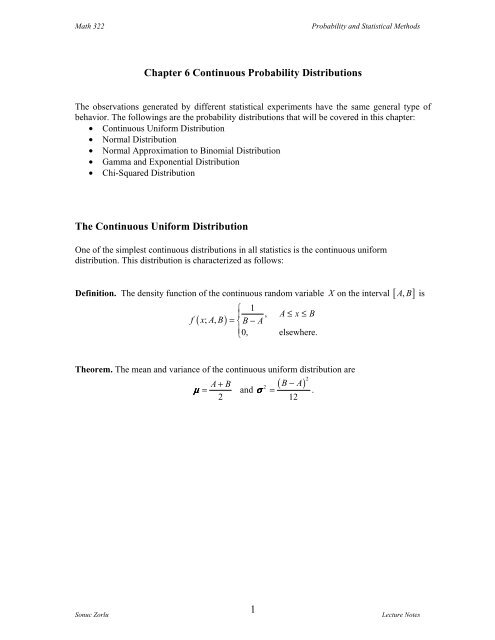
Chapter 6 Continuous Probability Distributions
The observations generated by different statistical experiments have the same general type of
behavior. The followings are the probability distributions that will be covered in this chapter:
• Continuous Uniform Distribution
• Normal Distribution
• Normal Approximation to Binomial Distribution
• Gamma and Exponential Distribution
• Chi-Squared Distribution
The Continuous Uniform Distribution
One of the simplest continuous distributions in all statistics is the continuous uniform
distribution. This distribution is characterized as follows:
Definition. The density function of the continuous random variable X on the interval [ A, B ] is
⎧ 1
⎪ , A ≤ x ≤ B
f ( x; A, B) = ⎨ B − A
⎪
⎩0,
elsewhere.
Theorem. The mean and variance of the continuous uniform distribution are
( ) 2
A + B
B − A
2
μμμμ = and σσσσ = .
2
12
1
Sonuc Zorlu Lecture Notes

Math 322 Probability and Statistical Methods
The Normal Distribution
The most important continuous probability distribution in the entire field of statistics is the
normal distribution. Normal distributions are a family of distributions that have the same general
shape. They are symmetric with scores more concentrated in the middle than in the tails. Normal
distributions are sometimes described as bell shaped which are shown below. Notice that they
differ in how spread out they are. The area under each curve is the same. The height of a normal
distribution can be specified mathematically in terms of two parameters: the mean (µ) and the
standard deviation (σ).
Definition. The density function of the normal random variable X , with mean μμμμ and variance
2
σσσσ , is
where ππππ = 3.14159.... and e = 2.71828 .
Standard normal distribution
2
1 −( 1/ 2 ) ⎡⎣ ( x−μμ
μμ ) / σσ
σσ
⎤⎦
N ( x; μμ μμ , σσ
σσ
) = e , − ∞ < x < ∞
2πσ
πσ πσ πσ
The standard normal distribution is a normal distribution with a mean of 0 and a standard
deviation of 1. Normal distributions can be transformed to standard normal distributions by the
formula:
where X is a score from the original normal distribution, µ is the mean of the original normal
distribution, and σ is the standard deviation of original normal distribution. The standard normal
distribution is sometimes called the z distribution. A z score always reflects the number of
standard deviations above or below the mean a particular score is. For instance, if a person
scored a 70 on a test with a mean of 50 and a standard deviation of 10, then they scored 2
standard deviations above the mean. Converting the test scores to z scores, an X of 70 would be:
2
Sonuc Zorlu Lecture Notes

Math 322 Probability and Statistical Methods
So, a z score of 2 means the original score was 2 standard deviations above the mean. Note that
the z distribution will only be a normal distribution if the original distribution (X) is normal.
Note : The following figures give us the areas to the right of some z − value, to the left of some
z − value and between two z − values.
Areas under portions of the standard normal distribution are shown to the right. About .68 (.34 +
.34) of the distribution is between -1 and 1 while about .96 of the distribution is between -2 and
2.
3
Sonuc Zorlu Lecture Notes

Math 322 Probability and Statistical Methods
Example 1. Given a standard normal distribution, find the area under the curve that lies
(a) to the right of z = 1.84
(b) between z = − 1.97 and z = 0.86
Solution. (a) P ( Z ) P ( Z )
by table A3
> 1.84 = 1− ≤ 1.84 = 1− 0.9671 = 0.0329 .
(b) P ( Z ) P ( Z ) P ( Z )
by table A3
− 1.97 < < 0.86 = < 0.86 − < − 1.97 = 0.8051− 0.0244 = 0.7807
Example 2. Given a normal distribution with μμμμ = 50 and σσσσ = 10 , find the probability that
X assumes a value between 45 and 62.
Solution.
⎛ 45 − 50 62 − 50 ⎞
P ( 45 < X < 62) = P⎜ < Z < ⎟ = P ( − 0.5 < Z < 1.2 ) = table(1.2) − table(
−0.5)
⎝ 10 10 ⎠
= 0.8849-0.3088 = 0.5764
Example 3. Given a standard normal distribution, find the value of k such that
(a) P( Z < k ) = 0.0427
(b) P ( Z > k ) = 0.2946
(c) P ( Z k )
− 0.93 < < = 0.7235
Solution. (a) P ( Z < k ) = 0.0427 ⇒ table( k) = 0.0427 ⇒ k = − 1.72
(b)
(c) ( )
( ) ( ) ( )
⇒ P ( Z ≤ k ) = 1− 0.2946 = 0.7054
P Z > k = 0.2946 ⇒ P Z > k = 1− P Z ≤ k = 0.2946
⇒ table( k) = 0.7054 ⇒ k = 0.54
P − 0.93 < Z < k = 0.7235 ⇒ table( k) − table(
− 0.93) = 0.7235
table( k)
= 0.7235 + 0.1762 = 0.8997
⇒ k = 1.28
Example 4. Given the normally distributed random variable X with μμμμ X = 18 and
(a) Compute P ( X > 13.74)
(b) Compute x satisfying P ( x X )
< < 18 = 0.4332 .
σσσσ = 3
4
Sonuc Zorlu Lecture Notes
2
X

Math 322 Probability and Statistical Methods
Applications of the normal Distribution
Example 1. A certain machine makes electrical resistors having a mean resistance of 40 ohms
and a standard deviation of 2 ohms. Assuming that the resistamce follows a normal distribution
and can be measured to any degree of accuracy, what percenatge of resistors wil have a
resistance exceeding 43 ohms?
Solution. Let X be the normal random variable, given μμ μμ = 40 ohms, σσ
σσ
= 2ohms
,
⎛ X − μμμμ 43 − 40 ⎞
P ( X > 43) = P ⎜ > ⎟ = P ( Z > 1.5) = 1− P ( Z ≤ 1.5)
⎝ σσσσ 2 ⎠
= 1 − table(1.5)
= 1− 0.9332 = 0.0668 = 6.68%
Example 2. The average grade for a exam is 74 and the standard deviation is 7. Assuming that
the grades follow a normal distribution, what is the probability that a student will get grade of at
least 60?
Normal Approximation to Binomial Distribution
2
Theorem. If X is a binomial random variable with mean μμμμ = np and σσσσ = npq , then the
limiting form of distribution of
X bin − np
Z = as n → ∞
npq
is the standard normal distribution N ( 0,1)
.
Note. We use the normal approximation to binomial distribution whenever p is not close to 0
and 1. If both np and nq are greater than or equal to 5, the approximation will be good.
Example 1. The probability that a patient recovers from a blood disease is 0.4. If 100 people are
known to have contracted this disease what is the probability that less than 30 survive?
Solution. Let X be the number of surviving people from blood disease.
Given n = 100 and p = 0.40 , μμμμ = np = 100*0.40 = 40 , σσσσ = 100 * 0.40 * 0.60 = 0.24 ,
⎛ X − np 29.5 − 40 ⎞
P ( X bin < 30) ≈ P ( X nor < 29.5) = P⎜ < = P ( Z < − 2.14 ) = table(
− 2.14) = 0.0162
⎜
⎟
npq 24 ⎟
⎝ ⎠
5
Sonuc Zorlu Lecture Notes

Math 322 Probability and Statistical Methods
6
Sonuc Zorlu Lecture Notes

Math 322 Probability and Statistical Methods
Example 2. A coin is tossed 400 times, use the normal approximation to binomial to find the
probability of obtaining
(a) between 185 and 210 heads inclusive
(b) exactly 205 heads
(c) less than 176 or more than 227 heads
Example 3. A ablanced die is rolled 180 times. Let be the number of cases when die shows the
number 4 on its top face.
(a) Find μμμμ X
(b) Find
2
σσσσ X
(c) Use normal approximation to binomial to approximate P ( 35 X 40)
Exercises
≤ ≤ .
Exercise1. If scores are normally distributed with a mean of 30 and a standard deviation of
5, what percent of the scores is: (a) greater than 30? (b) greater than 37? (c) between 28 and
34?
Exercise 2. Assume a normal distribution with a mean of 90 and a standard deviation of 7.
What limits would include the middle 65% of the cases?
Exercise 3. If is the standard normal random variable,
P − 1.3 < Z < 1.37
(a) Calculate ( )
(b) If P ( a Z 1.12) 0.6845
< < = , find the value of a .
Exercise 4. A research scientists reports that mice will live an average of 40 months when
their diets are sharply restricted and enriched with vitamins and proteins. Assuming that the
lifetimes of such mice are normally distributed with a standard deviation of 6.3 months, find
the probability that a given mouse will live
(a) more than 32 months
(b) less than 28 months
(c) between 37 and 49 months.
7
Sonuc Zorlu Lecture Notes

Math 322 Probability and Statistical Methods
Exponential and Gamma Distributions
Another continuous distribution that has many useful applications is the exponential distribution,
which has density
( )
f x
⎧ 1 −x
/ ββββ
⎪ e , x > 0
= ⎨ ββββ
⎪⎩ 0, elsewhere
Because the sample space for this distribution consists of the positive real numbers, this
distribution is sometimes used to model time to failure or survival time of a system. The
distribution function is,
x
1 −t / ββ ββ −x
/ ββ
ββ
F( x) = ∫ e dt = 1 − e , x > 0
ββββ
−∞
The exponential distribution has a special property that is unique to this distribution. Suppose
that T is the time to failure of a randomly selected new component, and suppose that this r.v. has
an exponential distribution with parameter ββββ . The probability that this new component survives
to time t is,
−t
/
( > ) = 1−
( ) =
P T t F t e
A generalization of the exponential distribution that can provide a much wider range of models is
f t; αα αα , β ββ
β by
based on the gamma integral. Define a function ( )
⎧ 1 αα αα −1 −x
/ ββ
ββ
⎪ x e , x ≥ 0
αααα
= ⎨Γ αα αα ββ
ββ
⎪⎩ 0, otherwise
( ; αα αα , ββ
ββ
) ( )
f x
where αα αα , β ββ
β are positive constants. Note that in this parameterizaton, the parameter ββββ is in the
denominator of the exponential component. The reason for this modification will be shown
below. Recall that
which implies that
and hence that f ( x; αα α, ββ
β )
∞
αα αα −1 −t
/ ββ ββ αα
αα
t e dt
∫
0
∞
∫
0
( αα αα ββ
ββ
)
8
Sonuc Zorlu Lecture Notes
( )
= ββ ββ Γ αα
αα
f t; , dt = 1
α β is a density function. This density function defines a distribution on
the positive real numbers and is referred to as the gamma distribution. Note that the
exponential distribution is a special case of the gamma distribution in whichαααα = 1.
The
parameter αααα is referred to as the shape parameter and ββββ is referred to as the scale parameter of
the gamma distribution.
ββββ

Math 322 Probability and Statistical Methods
Theorem. The Mean and Variance of the Gamma Distribution are
2 2
μμ μμ = αβ αβ αβ αβ and σσ σσ = αβ αβ αβ αβ
Theorem. The Mean and Variance of the Exponential Distribution are
2 2
μμ μμ = ββ
ββ
and σσ σσ = ββ
ββ
The following is the plot of the gamma probability density function.
Example 1. In a certain city the daily consumption of water (in millions of liters) follows a
gamma distribution with αααα = 2 and ββββ = 3 .If the daily capacity of that city is 9 million liters of
water, what is the probability that on a given day the water supply will be inadequate?
Solution. Let X be the water supply in millions of liters of water. Given αααα = 2 and ββββ = 3 ,
Thus, ( 9)
∞
⎧ 1 −x
/ 3
⎪ xe , x > 0
2
P( X > 9)
= ∫ f ( x) dx where f ( x)
= ⎨Γ ( 2) 3
9
⎪⎩ 0, otherwise
∞
− x / 3
P X xe dx
1 1
> = ∫ = . 3
9 e
9
Note. There is a relationship between the Exponential and Poisson distributions. Suppose events
are occurring in time according to Poisson distribution with a rate of λλλλ events per hour. Thus in
t hours, the number of events say Y , will have a Poisson distribution with mean value λλλλ t .
9
Sonuc Zorlu Lecture Notes

Math 322 Probability and Statistical Methods
10
Sonuc Zorlu Lecture Notes

Math 322 Probability and Statistical Methods
Suppose we start at time zero and ask the question ‘How long do I have to wait to see the first
event occur?’. Let X denote the length of time until the first event. Then
and
( ) ( )
( ) 0
> = = 0 int (0, )
−λλλλ
t
λλλλ t e
P X t P Y on the erval t
= = e
0!
11
Sonuc Zorlu Lecture Notes
−λλλλ
t
( ) ( )
t
P X t 1 P X t 1 e λλλλ −
≤ = − > = − .
Thus,
P X ≤ t = F t , the distribution function for X has the form of an exponential distribution
( ) ( )
1
with λλλλ = (the failure rate). Upon differentiating, we see that
ββββ
−λλλλ
t ( 1− ) 1 −t
/
d e
ββββ
f ( t) = = e , t > 0 .
dt ββββ
Example 2. The life of a certain type of device has an advertised rate of 0.01 per hour. The
failure rate is constant and the exponential dsitribution applies.
(a) What is the probability that 200-hours will pass before a failure is observed?
−0.01x
⎧ 0.01 e , x > 0
Solution. Given f ( x)
= ⎨ ,
⎩0,
otherwise
−0.01x −0.01x ∞ −2
( > ) = = − =
∫
P X 200 0.01 e dx e e .
200
(b) What is the mean time to failure?
Solution. Since the failure rate 1
= 0.01, μμ μμ = ββ
ββ
= 100 . Therefore the mean failure time is
ββββ
100-hours.
Example 3. The length of time for one individual to be served at a cafeteria is a random variable
having an exponential distribution with a mean of 4-minutes. What is the probability that a
person is served is less than 3-minutes on at least 4 of the next 6 days?
Example 4. The exponential distribution is frequently applied to the waiting times between
successes in a Poisson process. If the number of calls received per hour by a telephone answering
service is a Poisson random variable with parameter λλλλ = 6 , we know that the time, in hours,
1
between successive calls has an exponential distribution with parameter ββββ = . What is the
6
probability of waiting more than 15 minutes between any two successive calls?
Example 5. In a certain city, the daily consumption of electric power in millions of kw-hours is a
2
random variable X having a Gamma distribution with μμμμ = 6 and σσσσ = 12 .

Math 322 Probability and Statistical Methods
(a) Find the values of αααα and ββββ .
μμ μμ = αβ αβ αβ αβ = 6 ⎫
ββ ββ 2, αα
αα
3
2 2 ⎬ ⇒ = = .
σσ σσ = αβ αβ αβ αβ = 12 = 6.2⎭
(b) Find the probability that on any given day the daily power consumption will exceed 12
million kw-hours.
∞ ∞
1 −x / 2 2 1 − x / 2 2
P ( X > 12)
= ∫ e x dx = e x dx
3
12 2 Γ(
3)
16∫
12
Chi-Squared Distribution
Another very important special case of the Gamma distribution is obtained by letting αα αα = υυ
υυ
/ 2
and ββββ = 2 , where υυυυ is a positive integer. The result is called the Chi-squared distribution. The
distribution has a single parameter, υυυυ , called the degrees of freedom.
Definition. The continuous random variable X has a Chi-squared distribution, with υυυυ degrees
of freedom, if its densityfunctionis given by
⎧ 1 υυυυ / 2−1 − x / 2
⎪
x e , x > 0
υυυυ / 2
f ( x)
= ⎨2 Γ(
υυυυ / 2 )
⎪⎩ 0, elsewhere
where υυυυ is a positive integer.
The Chi-squared distribution plays a vital role in stsatistical inference that will be studied in the
next chapter. Topics dealing with sampling distributions, analysis of variance, and nonparametric
statistics involve extensive use of the Chi-squared distribution.
Theorem. The mean and variance of the Chi-squared distribution are
2
μμ μμ = υυ
υυ
and σσ σσ = 2υυ
υυ
.
12
Sonuc Zorlu Lecture Notes