Solutions - School of Mathematics and Statistics - Carleton University

CARLETON UNIVERSITY
SCHOOL OF MATHEMATICS AND STATISTICS
MATH2107 Linear Algebra II
Solutions to Test 2
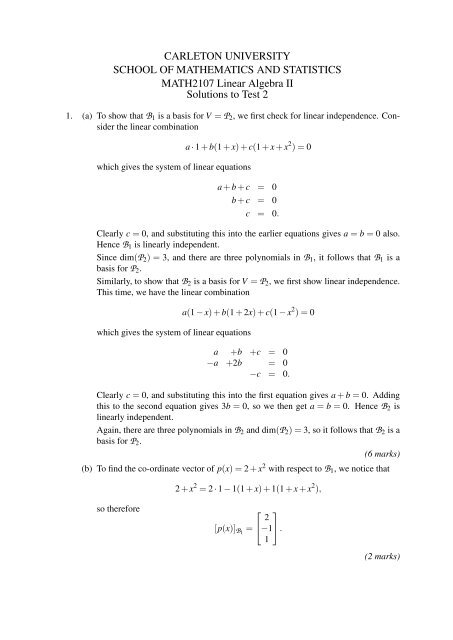
1. (a) To show that B1 is a basis for V = P2, we first check for linear independence. Consider
the linear combination
a · 1 + b(1 + x) + c(1 + x + x 2 ) = 0
which gives the system of linear equations
a + b + c = 0
b + c = 0
c = 0.
Clearly c = 0, and substituting this into the earlier equations gives a = b = 0 also.
Hence B1 is linearly independent.
Since dim(P2) = 3, and there are three polynomials in B1, it follows that B1 is a
basis for P2.
Similarly, to show that B2 is a basis for V = P2, we first show linear independence.
This time, we have the linear combination
a(1 − x) + b(1 + 2x) + c(1 − x 2 ) = 0
which gives the system of linear equations
a +b +c = 0
−a +2b = 0
−c = 0.
Clearly c = 0, and substituting this into the first equation gives a + b = 0. Adding
this to the second equation gives 3b = 0, so we then get a = b = 0. Hence B2 is
linearly independent.
Again, there are three polynomials in B2 and dim(P2) = 3, so it follows that B2 is a
basis for P2.
(6 marks)
(b) To find the co-ordinate vector of p(x) = 2 + x 2 with respect to B1, we notice that
so therefore
2 + x 2 = 2 · 1 − 1(1 + x) + 1(1 + x + x 2 ),
[p(x)]B1 =
⎡ ⎤
2
⎣−1⎦.
1
(2 marks)

(c) Let B1 be the matrix whose columns are the co-ordinate vectors of B1 with respect
to the standard basis, and likewise B2 the same matrix but for B2. So we have
⎡
1 1
⎤
1
B1 = ⎣0
1 1⎦
0 0 1
and
B2 =
⎡
1 1
⎤
1
⎣−1
2 0 ⎦.
0 0 −1
To use the Gauss–Jordan Method, we take the 3 × 6 matrix [B2 | B1], and apply
elementary row operations until the left-hand matrix is the identity:
⎡
1 1 1 1 1
⎤
1
⎡
1 1 1 1 1
⎤
1
⎣ −1 2 0 0 1 1 ⎦ ∼ ⎣ 0 3 1 1 2 2 ⎦
0 0 −1 0 0 1 0
⎡
1
0
1
−1
1
0
1
0
1
1
⎤
1
∼
∼
⎣ 0
0
⎡
1
⎣
1
0
0
1 1 2 2 ⎦
3 3 3 3
−1 0 0 1
2 0 1
2 1 1
3 3 3 3
1 ∼
0
⎡
1
⎣
0
0
⎤
1 2 2 ⎦
3 3 3 3
1 0 0 −1
0 2 0 1
1
3 3 1
0 1 0 0
⎤
2
3 3 1 ⎦
1 0 0 −1
So the change-of-basis matrix is the matrix on the right, i.e.
PB2←B1 =
⎡ 2
3
⎣ 1
3
0
1
3
2
3
0
⎤
1
1 ⎦.
−1
(7 marks)
(d) To find the co-ordinate vector of p(x) with respect to B2, we take the one we obtained
in (b) and multiply it by the change-of-basis matrix we obtained in (c):
[p(x)]B2
= PB2←B1 [p(x)]B1
⎡ 2 1
3 3
= ⎣
1
1 2
3 3 1
⎤⎡
⎤
2
⎦⎣−1⎦
0 0 1 1
⎡ ⎤
2
= ⎣ 1 ⎦.
−1
(2 marks)

2. (a) T (A) = trace(A) is a linear transformation from M33 to R, as both conditions hold.
For all matrices A,B and scalars c, we have
and
T (A + B) = (a11 + b11) + (a22 + b22) + (a33 + b33)
= (a11 + a22 + a33) + (b11 + b22 + b33)
= T (A) + T (B)
T (cA) = ca11 + ca22 + ca33
= c(a11 + a22 + a33)
= cT (A).
(b) The map T : M22 → M22 defined by
a
T
c
b c
=
d d
a
b
a
is a linear transformation. Let A =
c
b
x
and B =
d
z
y
. Then we have
w
T (A + B) =
=
=
a + x b + y
T
c + z d + w
c + z a + x
d + w b + y
c a z x
+
d b w y
and also
(where k is any scalar).
(c) The map T : M22 → M22 defined by
a b
T =
c d
= T (A) + T (B)
ka kb
T (kA) = T
kc kd
kc ka
=
kd kb
c a
= k
d b
= kT (A)
1
a + b
c + d −1
is not a linear transformation, since T (0) = 0: observe that
0
T
0
0 1
=
0 0
0 0
=
−1 0
0
.
0
(3 marks)
(3 marks)
(3 marks)

3. To show for any linear transformation T : V → W that T (0V ) = 0W , we start by choosing
any vector v ∈ V . Then (by a result about vector spaces), 0v = 0V . Applying T to both
sides of this, we have
T (0V ) = T (0v)
= 0T (v) (by the definition of a linear transformation)
= 0W
(since T (v) is a vector in W).
4. We have linear transformations T : M22 → P3 and S : P3 → R3 given by
a b
T = (a + b) + (a − b)x + (c − d)x
c d
2 + (c + d)x 3
and
S(a + bx + cx 2 + dx 3 ⎡ ⎤
2b
) = ⎣ a + c ⎦.
c − 2d
(a) To find the composition S ◦ T : M22 → R3
, we find S(T (A)) for a matrix
a b
A = :
c d
(S ◦ T )
a b
c d
= S((a + b) + (a − b)x + (c − d)x 2 + (c + d)x 3 )
⎡
2(a − b)
⎤
= ⎣ (a + b) + (c − d) ⎦
(c − d) − 2(c + d)
⎡
⎤
2a − 2b
= ⎣a
+ b + c − d⎦.
−c − 3d
1 2
(b) To find (S ◦ T ) , we use the formula we found in part (a):
0 −1
⎡
⎤ ⎡ ⎤
2 − 4 −2
1 2
(S ◦ T ) = ⎣1
+ 2 + 0 − (−1) ⎦ = ⎣ 4 ⎦.
0 −1
0 − (−3) 3
(5 marks)
(4 marks)
(1 mark)
(c) Now we have linear transformations F : M22 → P3 and G : P3 → M22 given by
a b
F = (a + b) + bx + (2c + d)x
c d
2 + cx 3
and
G(a + bx + cx 2 + dx 3 ) =
a − b b
.
d c − 2d

To show that F and G are inverses, we need to show that both G ◦ F = IM22 and
F ◦ G = IP3 .
First, we find the composition G ◦ F : M22 → M22. We have
a b
G ◦ F = G((a + b) + bx + (2c + d)x
c d
2 + cx 3 )
(a + b) − b b
=
c (2c + d) − 2c
a b
= ,
c d
so therefore G ◦ F = IM22 .
Second, we find the composition F ◦ G : P3 → P3. We have
F(G(a + bx + cx 2 + dx 3
a − b b
)) = F
d c − 2d
so therefore F ◦ G = IP3 .
Hence F and G are inverses.
5. (a) The kernel of T is the set
and the range of T is the set
= ((a − b) + b) + bx + (2d + (c − 2d))x 2 + dx 3
= a + bx + cx 2 + dx 3 ,
ker(T ) = {v ∈ V | T (v) = 0}
range(T ) = {w ∈ W | w = T (v) for some v ∈ V }.
(b) To show that the map T : M22 → R2 given by
a b a − b
T =
c d b + c
is a linear transformation, we consider matrices A =
Then we have
a + x b + y
T (A + B) = T
c + z d + w
(a + x) − (b + y)
=
(b + y) + (c + z)
(a − b) + (x − y)
=
(b + c) + (y + z)
a − b x − y
= +
b + c y + z
= T (A) + T (B)
a b
c d
and B =
(9 marks)
(2 marks)
x y
.
z w

and
(for some scalar k).
(c) The kernel of T is the set
ker(T ) =
=
=
=
ka kb
T (kA) = T
kc kd
ka − kb
=
kb + kc
a − b
= k
b + c
= kT (A)
a b a b 0
T =
c d c d 0
a b a − b 0
=
c d b + c 0
a b
a − b = 0, b + c = 0
c d
a a
a,d ∈ R .
−a d
(2 marks)
The range of T is all of R2 , since any vector in R2
is the image under T of some
x
matrix in M22. To show this, let v = ∈ R
y
2 . Then
x 0 x − 0 x
T = = ,
y 0 0 + y y
i.e. for any v ∈ R2
x 0
, there exists the matrix A = ∈ M22 satisfying T (A) = v.
y 0
(8 marks)
(d) The set
1 1
,
−1 0
0 0
0 1
is a basis for ker(T ). To check for linear independence, we consider the equation
1
a
−1
1 0
+ b
0 0
0 0
=
1 0
0
0
which gives a = 0 and b = 0. To check that it is a spanning set, we notice that any
matrix in the kernel can be written as
a a 1
= a
−a d −1
1 0
+ d
0 0
0
.
1
(3 marks)
Total marks: 60
R. F. Bailey, 14th July 2009