Populations, Parameters, Statistics, and Sampling

Populations, Parameters, Statistics,
and Sampling
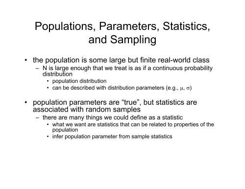
• the population is some large but finite real-world class
– N is large enough that we treat is as if a continuous probability
distribution
• population distribution
• can be described with distribution parameters (e.g., μ, σ)
• population parameters are “true”, but statistics are
associated with random samples
– there are many things we could define as a statistic
• what we want are statistics that can be related to properties of the
population
• infer population parameter from sample statistics

Sampling Distributions
• When taking N samples (observations) from the
population, we are interested in is a statistic across all
possible samples of N
– sampling distribution: for an assumed population parameter, the
probability distribution for all possible samples of size N
• e.g., sampling N times from a Bernoulli population with parameter P
• If N=1, the sampling distribution is the population distribution
– sampling distribution of the mean
• just like the population, sampling distributions are theoretical, and
have “true” parameters
– standard deviation of the sampling distribution of the mean is the
standard error of the mean (σ M )
• The statistics from a particular sample give a “point
estimation” for the population parameters
– in general these will be different due to random effects

Maximum Likelihood (MLE)
• In calculating an estimate of the population parameter, set
it so as to maximize the probability of the sample
observations
– p(D | M) is the likelihood of the data (D) given a population model
(M)
– an example:
• three hypotheses regarding proportion of liberal arts majors (.4, .5,
and .6)
• Sample 15 students and observe that 9 are liberal arts majors
• What’s the likelihood of each hypothesis?
– L(x=9; p=?, N=15)
– A statistic is a maximum likelihood estimator (MLE) when its value
as applied to population parameter maximizes the sample result

Other Properties
• Some statistics are designed with other properties in mind
beyond probability (MLE) – in these examples, G is
sample statistic that estimates θ
– unbiased
• expected value of G over all samples is θ (E[G] = θ)
– x is unbiased estimate of μ
– for binomial, P is unbiased estimate of p
– however, S 2 is a biased estimate of σ 2
– consistency
• as N increases, should approach population parameters
– relative efficiency
• the variance of the estimator as compared to other estimators
– mean is more efficient than median for normal distributions
– sufficient
• G contains all the information in the sample that can be used to find θ
– often a set of sufficient statistics is required (e.g., mean and corrected
variance)

Sampling Distribution of the Mean
• Mean is unbiased, consistent, efficient, and combined
with σ 2 is sufficient in many circumstances
– the mean of the sampling distribution of means is the same as
the population mean
• However, the sampling distribution of the mean is not
identical to population distribution
• for example, variance of means σ M 2 = σ 2 / N
– σ M is the standard error of the mean
– a standard score of the sample mean is therefore
Z
M
x − μ x − μ
= =
σ σ / N
M
– in order to compare the observed mean to the expected mean given
some hypothesis, we need the standard error of the mean
– suppose x = 15, μ = 10, σ = 4 and N = 16
» what’s the probability of this deviant, or greater?

• E[S 2 ] ≠ σ 2
Bias in the Sample Variance
– proof on p. 216 E[S2 ] = σ2 - σ 2
M
• this is because the mean used to calculate S will in general be
different than the population mean
– the sample mean is always exactly centered on the particular sample
and so deviations from it underestimate true population deviations
2
2 2 2 2 σ ⎛ N −1
⎞ 2
ES [ ] = σ − σM= σ − = ⎜ ⎟σ
N ⎝ N ⎠
– the sample variance is too small by a factor of (N-1)/N
• S 2 is the uncorrected variance and s 2 is corrected
– the corrected standard deviation is still slightly biased (only variance
is unbiased)
» the amount of remaining bias is small though, so it’s typical to
use s to estimate σ
• unbiased estimate of standard error of the mean
ˆ σ M =
ˆ σ
=
N
s
=
N
S
N −1

Other Issues with Estimators
• Pooling two or more samples results in better estimation
– frequency weighted average (pp. 219-220)
• For small populations, can’t assume sampling with
replacement, and so the estimates need to be slightly
larger (p.220)
• Because the sample mean is typically different than the
population mean, it’s useful to define a confidence
interval for the population mean
– using Tchebycheff inequality, the sample mean is between x
±
kσ M with at least probability 1 – (1/k 2 )
• this is not the probability that x is μ
– the probability that the interval from this sample covers μ
• this is a very rough estimate and additional assumptions regarding
the sampling distribution tighten the estimate
– for unimodal symmetric sampling distribution, 95% interval with k=3