Identifying Stored-Grain Insects Using Near-Infrared Spectroscopy

More documents

Recommendations

Info

166 JOURNAL OF ECONOMIC ENTOMOLOGY Vol. 92, no. 1 Table 1. <strong>Stored</strong>-grain beetles (Coleoptera) used in the neural network and partial least squares analysis of NIR spectra when comparing species, genera, and primary versus secondary pests Code Common name ScientiÞc name Family FGB Flat grain beetle Secondary Pests Cryptolestes pusillus (Schönherr) Laemophloeidae RGB Rusty grain beetle Cryptolestes ferrugineus (Stephens) Laemophloeidae SGB Sawtoothed grain beetle Oryzaephilus surinamensis (L.) Silvanidae MGB Merchant grain beetle Oryzaephilus mercator (Fauvel) Silvanidae CFB Confused ßour beetle Tribolium confusum Jacquelin du Val Tenebrionidae RFB Red ßour beetle Tribolium castaneum (Herbst) Primary Pests Tenebrionidae LGB Lesser grain borer Rhyzopertha dominica (F.) Bostrichidae GB Larger grain borer Prostephanus truncatus (Horn) Bostrichidae GW Granary weevil Sitophilus granarius (L.) Curculionidae RW Rice weevil Sitophilus oryzae (L.) Curculionidae MW Maize weevil Sitophilus zeamais Motschulsky Curculionidae Materials and Methods About 20 adult insects were selected from each of 11 beetle species commonly found in stored grain (Table 1). These species were obtained from stock colonies reared at 25 o C and 50Ð60% RH. Composition of laboratory diets for the different species were as follows: diets for the ßat grain beetle, Cryptolestes pusillus (Schönherr) (Coleoptera: Laemophloeidae); rusty grain beetle; sawtoothed grain beetle, Oryzaephilus surinamensis (L.) (Coleoptera: Silvanidae); and merchant grain beetle, Oryzaephilus mercator (Fauvel) (Coleoptera: Silvanidae), consisted of oatmeal: whole wheat ßour:BrewerÕs yeast:wheat germ (60:30: 5:5), (vol:vol); diets for the confused ßour beetle, Tribolium confusum Jacquelin du Val (Coleoptera: Tenebrionidae), and the red ßour beetle, Tribolium castaneum (Herbst) (Coleoptera: Tenebrionidae), consisted of whole wheat ßour and BrewerÕs yeast (95:5), (vol:vol); the lesser grain borer was reared on whole wheat lightly dusted with wheat ßour; the larger grain borer, Prostephanus truncatus (Horn) (Coleoptera: Bostrichidae), and the maize weevil, Sitophilus zeamais Motschulsky (Coleoptera: Curculionidae), were reared on whole-kernel corn; and the rice weevil, Sitophilus oryzae (L.) (Coleoptera: Curculionidae), and granary weevil, Sitophilus granarius (L.) (Coleoptera: Curculionidae), were reared on hard red winter wheat. The live insects were individually placed in a black V-shaped trough (12 mm long, 10 mm wide, 5 mm deep) and illuminated with white light via a Þber bundle (8 mm diameter) positioned 13 mm from the top of the trough and oriented 45 o from vertical. A reßectance probe (2-mm diameter) was oriented vertically 9.5 mm from the top of the trough. The reßectance probe carried the reßected energy to a spectrometer (DA7000, Perten Instruments, SpringÞeld, IL). The diode-array spectrometer measures visible (400Ð750 nm) and NIR (750Ð1,700 nm) reßectance at a rate of 30 spectra per second. Procedures included collecting a baseline, collecting 8 spectra from each of the insects, and averaging the 8 spectra for each insect. This resulted in spectra from 275 individual insects. Collecting and averaging the 8 spectra from each insect took 1 s. The baseline consisted of collecting a spectrum of the empty trough to use as a reference. A new baseline was collected after each group of 40 insects. Data were analyzed using partial least squares regression (PLS) (Galactic Industries 1996) and a backpropagation neural network (NeuralWare 1995). Correlation plots (r 2 ) and factors indicating which wavelengths contribute to classiÞcations in 2-way comparisons were obtained using PLS (Murray and Williams 1990). Two-way comparisons were made using PLS by assigning a value of 1 or 2 to the comparisons of interest (for example, primary 1, secondary 2). The neural network analysis gave classiÞcation percentages for all 2-way as well as higher-order comparisons (up to 11 species compared). The neural network had 1 hidden layer, 100 input nodes, and 2, 3, or 11 outputs. The 100-input nodes corresponded to the absorbance values at 10 nm increments from 700 to 1,700 nm. The outputs corresponded to the comparisons being tested. The learning rate, momentum, and learning events used in the neural network were 0.6, 0.4Ð0.5, and 10,000Ð30,000, respectively. The learning rate, momentum, learning events, and number of hidden layers affect the neural network accuracy and speed (Hecht-Neilsen 1989). For both the PLS and neural network analyses, even-numbered samples served as training or calibration sets, whereas odd samples were used for testing calibration models. Table 2 shows the comparisons tested. The classi- Þcation of paramount interest was primary versus secondary insects because management strategies for these 2 types of insects may be quite different and because knowing whether an insect is a primary or secondary pest is usually sufÞcient for making a management decision. In addition, insects were classed into their respective genera (2 or 3 comparisons) within the primary and secondary groupings, and classed into species within a genus (2 or 3 comparisons). A Þnal comparison sought to classify insects into their respective species independent of previous groupings (11 comparisons).
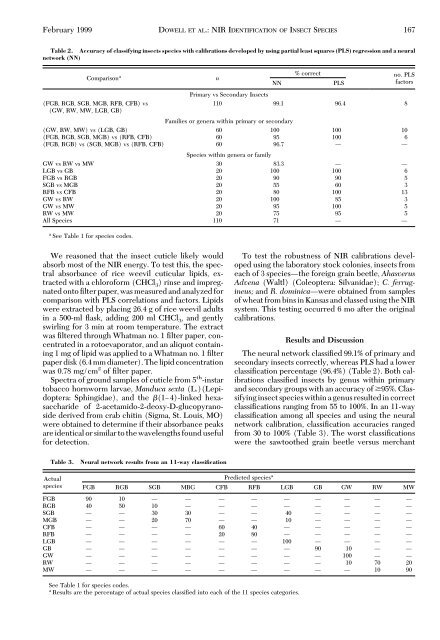
February 1999 DOWELL ET AL.: NIR IDENTIFICATION OF INSECT SPECIES 167 Table 2. Accuracy of classifying insects species with calibrations developed by using partial least squares (PLS) regression and a neural network (NN) Comparisona n Primary vs Secondary <strong>Insects</strong> NN % correct PLS no. PLS factors (FGB, RGB, SGB, MGB, RFB, CFB) vs (GW, RW, MW, LGB, GB) 110 99.1 96.4 8 Families or genera within primary or secondary (GW, RW, MW) vs (LGB, GB) 60 100 100 10 (FGB, RGB, SGB, MGB) vs (RFB, CFB) 60 95 100 6 (FGB, RGB) vs (SGB, MGB) vs (RFB, CFB) 60 96.7 Ñ Ñ GW vs RW vs MW Species within genera or family 30 83.3 Ñ Ñ LGB vs GB 20 100 100 6 FGB vs RGB 20 90 90 5 SGB vs MGB 20 55 60 3 RFB vs CFB 20 80 100 13 GW vs RW 20 100 85 3 GW vs MW 20 95 100 5 RW vs MW 20 75 95 5 All Species 110 71 Ñ Ñ a See Table 1 for species codes. We reasoned that the insect cuticle likely would absorb most of the NIR energy. To test this, the spectral absorbance of rice weevil cuticular lipids, extracted with a chloroform (CHCl 3) rinse and impregnated onto Þlter paper, was measured and analyzed for comparison with PLS correlations and factors. Lipids were extracted by placing 26.4 g of rice weevil adults in a 500-ml ßask, adding 200 ml CHCl 3, and gently swirling for 3 min at room temperature. The extract was Þltered through Whatman no. 1 Þlter paper, concentrated in a rotoevaporator, and an aliquot containing 1 mg of lipid was applied to a Whatman no. 1 Þlter paper disk (6.4 mm diameter). The lipid concentration was 0.78 mg/cm 2 of Þlter paper. Spectra of ground samples of cuticle from 5 th -instar tobacco hornworm larvae, Manduca sexta (L.)(Lepidoptera: Sphingidae), and the (1Ð4)-linked hexasaccharide of 2-acetamido-2-deoxy-D-glucopyranoside derived from crab chitin (Sigma, St. Louis, MO) were obtained to determine if their absorbance peaks are identical or similar to the wavelengths found useful for detection. Table 3. Neural network results from an 11-way classification Actual species To test the robustness of NIR calibrations developed using the laboratory stock colonies, insects from each of 3 speciesÑthe foreign grain beetle, Ahasverus Advena (Waltl) (Coleoptera: Silvanidae); C. ferrugineus; and R. dominicaÑwere obtained from samples of wheat from bins in Kansas and classed using the NIR system. This testing occurred 6 mo after the original calibrations. Results and Discussion The neural network classiÞed 99.1% of primary and secondary insects correctly, whereas PLS had a lower classiÞcation percentage (96.4%) (Table 2). Both calibrations classiÞed insects by genus within primary and secondary groups with an accuracy of 95%. Classifying insect species within a genus resulted in correct classiÞcations ranging from 55 to 100%. In an 11-way classiÞcation among all species and using the neural network calibration, classiÞcation accuracies ranged from 30 to 100% (Table 3). The worst classiÞcations were the sawtoothed grain beetle versus merchant Predicted species a FGB RGB SGB MBG CFB RFB LGB GB GW RW MW FGB 90 10 Ñ Ñ Ñ Ñ Ñ Ñ Ñ Ñ Ñ RGB 40 50 10 Ñ Ñ Ñ Ñ Ñ Ñ Ñ Ñ SGB Ñ Ñ 30 30 Ñ Ñ 40 Ñ Ñ Ñ Ñ MGB Ñ Ñ 20 70 Ñ Ñ 10 Ñ Ñ Ñ Ñ CFB Ñ Ñ Ñ Ñ 60 40 Ñ Ñ Ñ Ñ Ñ RFB Ñ Ñ Ñ Ñ 20 80 Ñ Ñ Ñ Ñ Ñ LGB Ñ Ñ Ñ Ñ Ñ Ñ 100 Ñ Ñ Ñ Ñ GB Ñ Ñ Ñ Ñ Ñ Ñ Ñ 90 10 Ñ Ñ GW Ñ Ñ Ñ Ñ Ñ Ñ Ñ Ñ 100 Ñ Ñ RW Ñ Ñ Ñ Ñ Ñ Ñ Ñ Ñ 10 70 20 MW Ñ Ñ Ñ Ñ Ñ Ñ Ñ Ñ Ñ 10 90 See Table 1 for species codes. a Results are the percentage of actual species classiÞed into each of the 11 species categories.
Page 1: SAMPLING AND BIOSTATISTICS Identify
Page 5: February 1999 DOWELL ET AL.: NIR ID

Identifying Stored-Grain Insects Using Near-Infrared Spectroscopy

Create successful ePaper yourself

Delete template?

Save as template?