EL-506W EL-546W - Sharp Australia Support

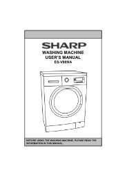
SCIENTIFIC CALCULATOR 

PRINTED IN CHINA / IMPRIMÉ EN CHINE / IMPRESO EN CHINA 

04HGK (TINSE0719EH01) 

INTRODUCTION 

Thank you for purchasing the SHARP Scientific Calculator Model 

EL-506W/546W. 

About the calculation examples (including some formulas and 

tables), refer to the reverse side of this English manual. Refer to 

the number on the right of each title in the manual for use. 

After reading this manual, store it in a convenient location for 

future reference. 

Note: Some of the models described in this manual may not be 

available in some countries. 

Operational Notes 

• Do not carry the calculator around in your back pocket, as it 

may break when you sit down. The display is made of glass 

and is particularly fragile. 

• Keep the calculator away from extreme heat such as on a car 

dashboard or near a heater, and avoid exposing it to excessively 

humid or dusty environments. 

• Since this product is not waterproof, do not use it or store it 

where fluids, for example water, can splash onto it. Raindrops, 

water spray, juice, coffee, steam, perspiration, etc. will also 

cause malfunction. 

• Clean with a soft, dry cloth. Do not use solvents or a wet cloth. 

• Do not drop it or apply excessive force. 

• Never dispose of batteries in a fire. 

• Keep batteries out of the reach of children. 

• This product, including accessories, may change due to upgrading 

without prior notice. 

NOTICE 

• SHARP strongly recommends that separate permanent 

written records be kept of all important data. Data may be 

lost or altered in virtually any electronic memory product 

under certain circumstances. Therefore, SHARP assumes 

no responsibility for data lost or otherwise rendered unusable 

whether as a result of improper use, repairs, defects, battery 

replacement, use after the specified battery life has expired, 

or any other cause. 

• SHARP will not be liable nor responsible for any incidental or 

consequential economic or property damage caused by 

misuse and/or malfunctions of this product and its peripherals, 

unless such liability is acknowledged by law. 

♦ Press the RESET switch (on the back), with the tip of a ballpoint 

pen or similar object, only in the following cases. Do not 

use an object with a breakable or sharp tip. Note that pressing 

the RESET switch erases all data stored in memory. 

• When using for the first time 

• After replacing the batteries 

• To clear all memory contents 

• When an abnormal condition occurs and all keys are inoperative. 

If service should be required on this calculator, use only a SHARP 

servicing dealer, SHARP approved service facility, or SHARP 

repair service where available. 

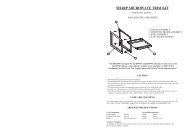
Hard Case 

DISPLAY 

Equation→ 

Display 

ENGLISH 

MODEL 

OPERATION MANUAL 

EL-506W 


←Symbol 

Mantissa Exponent 

• During actual use, not all symbols are displayed at the same time. 

• Certain inactive symbols may appear visible when viewed from 

a far off angle. 

• Only the symbols required for the usage under instruction are 

shown in the display and calculation examples of this manual. 

/ : Appears when the entire equation cannot be displayed. 

Press to see the remaining (hidden) section. 

xy/rθ : Indicates the mode of expression of results in the complex 

calculation mode. 

: Indicates that data can be visible above/below the 

screen. Press [/] to scroll up/down the view. 

2ndF : Appears when @ is pressed. 

HYP : Indicates that h has been pressed and the hyperbolic 

functions are enabled. If @H are pressed, 

the symbols “2ndF HYP” appear, indicating that inverse 

hyperbolic functions are enabled. 

ALPHA : Appears when K (STAT VAR), O or R is pressed. 

FIX/SCI/ENG: Indicates the notation used to display a value. 

DEG/RAD/GRAD: Indicates angular units. 

: Appears when matrix mode is selected. 

: Appears when list mode is selected. 

: Appears when statistics mode is selected. 

M : Indicates that a value is stored in the independent memory. 

? : Indicates that the calculator is waiting for a numerical 

value to be entered, such as during simulation calculation. 

: Appears when the calculator shows an angle as the result 

in the complex calculation mode. 

i : Indicates an imaginary number is being displayed in the 

complex calculation mode. 

BEFORE USING THE CALCULATOR 

Key Notation Used in this Manual 

In this manual, key operations are described as follows: 

To specify ex : @e 

To specify ln : I 

To specify F : Kü 

Functions that are printed in orange above the key require @ to 

be pressed first before the key. When you specify the memory, 

press K first. Numbers for input value are not shown as keys, 

but as ordinary numbers. 

Power On and Off 

Press ª to turn the calculator on, and @F to turn it off. 

Clearing the Entry and Memories 

Operation Entry M A-F, X,Y STAT* 1 matA-D* 3 

(Display) F1-F4 ANS STAT VAR* 2 L1-4* 4 

ª × × × × 

@c × 

Mode selection 

@∏00* 

× 

5 

@∏10* 6 

RESET switch 

: Clear × : Retain 

* 1 Statistical data (entered data). 

* 2 x¯, sx, σx, n, Σx, Σx 2 , ¯y, sy, σy, Σy, Σy 2 , Σxy, r, a, b, c. 

* 3 Matrix memories (matA, matB, matC and matD) 

* 4 List memories (L1, L2, L3 and L4) 

* 5 All variables are cleared. 

* 6 This key combination functions the same as the RESET switch. 

[Memory clear key] 

Press @∏ to display the menu. 

• To clear all variables (M, A-F, X, Y, ANS, 

MEM RESET 

0 1 

• 

F1-F4, STAT VAR, matA-D, L1-4), press 00 or 0 

®. 

To RESET the calculator, press 10 or 1®. 

The RESET operation will erase all data stored in memory, and 

restore the calculator’s default setting. 

Entering and Correcting the Equation 

[Cursor keys] 

• Press < or > to move the cursor. You can also return to 

the equation after getting an answer by pressing > (

the integral values during 

minute shifting of the integral 

range and for periodic 

y 

functions, etc., where positive 

and negative integral 

values exist depending on 

x 

y 

0 x 2 

the interval. 

b 

For the former case, divide a b 

x a 

x 

integral intervals as small 

x0 x1 xx 

x x 

2 

1 3 

as possible. For the latter 

3 

case, separate the positive and negative values. Following these 

tips will allow results of calculations with greater accuracy and will 

also shorten the calculation time. 

Random Function 

The Random function has four settings for use in the normal, statistics, 

matrix and list modes. (This function cannot be selected while 

using the N-Base function.) To generate further random numbers in 

succession, press ®. Press ª to exit. 

• The generated pseudo-random number series is stored in memory 

Y. Each random number is based on a number series. 

[Random Numbers] 

A pseudo-random number, with three significant digits from 0 up to 

0.999, can be generated by pressing @`0®. 

[Random Dice] 

To simulate a die-rolling, a random integer between 1 and 6 can be 

generated by pressing @`1®. 

[Random Coin] 

To simulate a coin flip, 0 (head) or 1 (tail) can be randomly generated 

by pressing @`2®. 

[Random Integer] 

An integer between 0 and 99 can be generated randomly by pressing 

@`3®. 

Angular Unit Conversions 

Each time @g are pressed, the angular unit changes in sequence. 

Memory Calculations 

Mode 

NORMAL 

ANS M, F1-F4 A-F, X,Y 

STAT × × 

EQN × × × 

CPLX × 

MAT × 

LIST × 

: Available × : Unavailable 

[Temporary memories (A-F, X and Y)] 

Press O and a variable key to store a value in memory. 

Press R and a variable key to recall a value from the memory. 

To place a variable in an equation, press K and a variable key. 

[Independent memory (M)] 

In addition to all the features of temporary memories, a value can 

be added to or subtracted from an existing memory value. 

Press ªOM to clear the independent memory (M). 

[Last answer memory (ANS)] 

The calculation result obtained by pressing = or any other 

calculation ending instruction is automatically stored in the last 

answer memory. A Matrix/List format result is not stored. 

[Formula memories (F1-F4)] 

Formulas up to 256 characters in total can be stored in F1 - F4. 

(Functions such as sin, etc., will be counted as one letter.) Storing 

a new equation in each memory will automatically replace the 

existing equation. 

Note: 

• Calculation results from the functions indicated below are automatically 

stored in memories X or Y replacing existing values. 

• Random function .......... Y memory 

• →rθ, →xy ........................ X memory (r or x), Y memory (θ or y) 

• Use of R or K will recall the value stored in memory using 

up to 14 digits. 

Chain Calculations 

• The previous calculation result can be used in the subsequent 

calculation. However, it cannot be recalled after entering multiple 

instructions or when the calculation result is in Matrix/List format. 

• When using postfix functions (¿ , sin, etc.), a chain calculation is 

possible even if the previous calculation result is cleared by the 

use of the ª key. 

Fraction Calculations 

Arithmetic operations and memory calculations can be performed 

using fractions, and conversion between a decimal number and a 

fraction. 

• If the number of digits to be displayed is greater than 10, the 

number is converted to and displayed as a decimal number. 

Binary, Pental, Octal, Decimal, and Hexadecimal 

Operations (N-Base) 

Conversions can be performed between N-base numbers. The four 

basic arithmetic operations, calculations with parentheses and 

memory calculations can also be performed, along with the logical 

operations AND, OR, NOT, NEG, XOR and XNOR on binary, pental, 

octal and hexadecimal numbers. 

Conversion to each system is performed by the following keys: 

@ê (“ ” appears.), @û (“ ” appears.), @î 

(“ ” appears.), @ì (“ ” appears.), @í (“ ”, “ ”, “ ” 

and “ ” disappear.) 

Note: The hexadecimal numbers A – F are entered by pressing 

ß, , L, ÷, l, and I, and displayed 

as follows: 

A → ï, B → ∫, C → ó, D → ò, E → ô, F → ö 

In the binary, pental, octal, and hexadecimal systems, fractional 

parts cannot be entered. When a decimal number having a fractional 

part is converted into a binary, pental, octal, or hexadecimal 

number, the fractional part will be truncated. Likewise, when 

the result of a binary, pental, octal, or hexadecimal calculation 

includes a fractional part, the fractional part will be truncated. In 

the binary, pental, octal, and hexadecimal systems, negative numbers 

are displayed as a complement. 

Time, Decimal and Sexagesimal Calculations 

Conversion between decimal and sexagesimal numbers can be 

performed, and, while using sexagesimal numbers, conversion to 

seconds and minutes notation. The four basic arithmetic operations 

and memory calculations can be performed using the 

sexagesimal system. Notation for sexagesimal is as follows: 

degree second 

minute 

Coordinate Conversions 

• Before performing a calculation, select the angular unit. 

P (x,y ) 

• The calculation result is automatically stored in memories X 

and Y. 

• Value of r or x: X memory • Value of θ or y: Y memory 

Calculations Using Physical Constants 

See the quick reference card and the English manual reverse side. 

A constant is recalled by pressing ß followed by the number 

of the physical constant designated by a 2-digit number. 

The recalled constant appears in the display mode selected with 

the designated number of decimal places. 

Physical constants can be recalled in the normal mode (when not 

set to binary, pental, octal, or hexadecimal), statistics mode, equation 

mode, matrix mode and list mode. 

Note: Physical constants and metric conversions are based either 

on the 2002 CODATA recommended values or 1995 Edition 

of the “Guide for the Use of the International System of 

Units (SI)” released by NIST (National Institute of Standards 

and Technology) or on ISO specifications. 

No. Constant 

No. Constant 

01 Speed of light in vacuum 

02 Newtonian constant of gravitation 

03 Standard acceleration of gravity 

04 Electron mass 

05 Proton mass 

06 Neutron mass 

07 Muon mass 

08 Atomic mass unit-kilogram 

relationship 

09 Elementary charge 

10 Planck constant 

11 Boltzmann constant 

12 Magnetic constant 

13 Electric constant 

14 Classical electron radius 

15 Fine-structure constant 

16 Bohr radius 

17 Rydberg constant 

18 Magnetic flux quantum 

19 Bohr magneton 

20 Electron magnetic moment 

21 Nuclear magneton 

22 Proton magnetic moment 

23 Neutron magnetic moment 

24 Muon magnetic moment 

25 Compton wavelength 

26 Proton Compton wavelength 

27 Stefan-Boltzmann constant 

y 

0 

Y 

x 

X 

↔ 

P (r,θ ) 

Rectangular coord. Polar coord. 

28 Avogadro constant 

29 Molar volume of ideal gas 

(273.15 K, 101.325 kPa) 

30 Molar gas constant 

31 Faraday constant 

32 Von Klitzing constant 

33 Electron charge to mass quotient 

34 Quantum of circulation 

35 Proton gyromagnetic ratio 

36 Josephson constant 

37 Electron volt 

38 Celsius Temperature 

39 Astronomical unit 

40 Parsec 

41 Molar mass of carbon-12 

42 Planck constant over 2 pi 

43 Hartree energy 

44 Conductance quantum 

45 Inverse fine-structure constant 

46 Proton-electron mass ratio 

47 Molar mass constant 

48 Neutron Compton wavelength 

49 First radiation constant 

50 Second radiation constant 

51 Characteristic impedance of 

vacuum 

52 Standard atmosphere 

Metric Conversions 

See the quick reference card and the English manual reverse side. 

Unit conversions can be performed in the normal mode (when not 

set to binary, pental, octal, or hexadecimal), statistics mode, equation 

mode, matrix mode and list mode. 

No. Remarks 

1 in : inch 

2 cm : centimeter 

3 ft : foot 

4 m : meter 

5 yd : yard 

6 m : meter 

7 mile : mile 

8 km : kilometer 

9 n mile : nautical mile 

10 m : meter 

11 acre : acre 

12 m 2 : square meter 

13 oz : ounce 

14 g : gram 

15 lb : pound 

16 kg : kilogram 

17 °F : Degree Fahrenheit 

18 °C : Degree Celsius 

19 gal (US) : gallon (US) 

20 l : liter 

21 gal (UK) : gallon (UK) 

22 l : liter 

0 

Y 

θ 

r 

No. Remarks 

23 fl oz(US) : fluid ounce(US) 

24 ml : milliliter 

25 fl oz(UK) : fluid ounce(UK) 

26 ml : milliliter 

27 J : Joule 

28 cal : calorie 

29 J : Joule 

30 cal15 : Calorie (15n°C) 

31 J : Joule 

32 calIT : I.T. calorie 

33 hp : horsepower 

34 W : watt 

35 ps : French horsepower 

36 W : watt 

37 

38 Pa : Pascal 

39 atm : atmosphere 


41 (1 mmHg = 1 Torr) 


43 

44 J : Joule 

X

Calculations Using Engineering Prefixes 

Calculation can be executed in the normal mode (excluding Nbase) 

using the following 9 types of prefixes. 

Prefix Operation Unit 

k (kilo) ∑10 10 3 

M (Mega) ∑11 10 6 

G (Giga) ∑12 10 9 

T (Tera) ∑13 10 12 

m (milli) ∑14 10 –3 

µ (micro) ∑15 10 –6 

n (nano) ∑16 10 –9 

p (pico) ∑17 10 –12 

f (femto) ∑18 10 –15 

Modify Function 

Calculation results are internally obtained in scientific notation 

with up to 14 digits for the mantissa. However, since calculation 

results are displayed in the form designated by the display notation 

and the number of decimal places indicated, the internal 

calculation result may differ from that shown in the display. By 

using the modify function, the internal value is converted to match 

that of the display, so that the displayed value can be used 

without change in subsequent operations. 

Solver Function 

The x value can be found that reduces an entered equation to “0”. 

• This function uses Newton's method to obtain an approximation. 

Depending on the function (e.g. periodic) or start value, an 

error may occur (Error 2) due to there being no convergence to 

the solution for the equation. 

• The value obtained by this function may include a margin of 

error. If it is larger than acceptable, recalculate the solution 

after changing ‘Start’ and dx values. 

• Change the ‘Start’ value (e.g. to a negative value) or dx value 

(e.g. to a smaller value) if: 

• no solution can be found (Error 2). 

• more than two solutions appear to be possible (e.g. a cubic 

equation). 

• to improve the arithmetic precision. 

• The calculation result is automatically stored in the X memory. 

[Performing Solver function] 

Q Press m0. 

W Input a formula with an x variable. 

E Press ∑0. 

R Input ‘Start’ value and press ®. The default value is “0”. 

T Input dx value (minute interval). 

Y Press ®. 

SIMULATION CALCULATION (ALGB) 

If you have to find a value consecutively using the same formula, 

such as plotting a curve line for 2x 2 + 1, or finding the variable for 

2x + 2y =14, once you enter the equation, all you have to do is to 

specify the value for the variable in the formula. 

Usable variables: A-F, M, X and Y 

Unusable functions: Random function 

• Simulation calculations can only be executed in the normal 

mode. 

• Calculation ending instructions other than = cannot be used. 

Performing Calculations 

Q Press m0. 

W Input a formula with at least one variable. 

E Press @≤. 

R Variable input screen will appear. Input the value of the flashing 

variable, then press ® to confirm. The calculation result will 

be displayed after entering the value for all used variables. 

• Only numerical values are allowed as variables. Input of 

formulas is not permitted. 

• Upon completing the calculation, press @≤ to perform 

calculations using the same formula. 

• Variables and numerical values stored in the memories will 

be displayed in the variable input screen. To change a 

numerical value, input the new value and press ®. 

• Performing simulation calculation will cause memory locations 

to be overwritten with new values. 

STATISTICAL CALCULATIONS 

Press m1 to select the statistics mode. The seven statistical 

calculations listed below can be performed. After selecting the 

statistics mode, select the desired sub-mode by pressing the 

number key corresponding to your choice. 

To change statistical sub-mode, reselect statistics mode (press 

m1), then select the required sub-mode. 

0 (SD) : Single-variable statistics 

1 (LINE) : Linear regression calculation 

2 (QUAD) : Quadratic regression calculation 

3 (EXP) : Exponential regression calculation 

4 (LOG) : Logarithmic regression calculation 

5 (PWR) : Power regression calculation 

6 (INV) : Inverse regression calculation 

The following statistics can be obtained for each statistical calculation 

(refer to the table below): 

Single-variable statistical calculation 

Statistics of Q and value of the normal probability function 

Linear regression calculation 

Statistics of Q and W and, in addition, estimate of y for a given 

x (estimate y´) and estimate of x for a given y (estimate x´) 

Exponential regression, Logarithmic regression, 

Power regression, and Inverse regression calculation 

Statistics of Q and W. In addition, estimate of y for a given x and 

estimate of x for a given y. (Since the calculator converts each 

formula into a linear regression formula before actual calculation 

takes place, it obtains all statistics, except coefficients a and b, 

from converted data rather than entered data.) 

Quadratic regression calculation 

Statistics of Q and W and coefficients a, b, c in the quadratic 

regression formula (y = a + bx + cx2 ). (For quadratic regression 

calculations, no correlation coefficient (r) can be obtained.) When 

there are two x´ values, press @≠. 

When performing calculations using a, b and c, only one numeric 

value can be held. 

¯x Mean of samples (x data) 

sx Sample standard deviation (x data) 

Q 

σx 

n 

Population standard deviation (x data) 

Number of samples 

Σx Sum of samples (x data) 

Σx 2 Sum of squares of samples (x data) 

¯y Mean of samples (y data) 

sy Sample standard deviation (y data) 

σy Population standard deviation (y data) 

Σy Sum of samples (y data) 

W Σy 2 Sum of squares of samples (y data) 

Σxy Sum of products of samples (x, y) 

r Correlation coefficient 

a Coefficient of regression equation 

b Coefficient of regression equation 

c Coefficient of quadratic regression equation 

• Use K and R to perform a STAT variable calculation. 

Data Entry and Correction 

Entered data are kept in memory until @c or mode selection. 

Before entering new data, clear the memory contents. 

[Data Entry] 

Single-variable data 

Data k 

Data & frequency k (To enter multiples of the same data) 

Two-variable data 

Data x & Data y k 

Data x & Data y & frequency k (To enter multiples 

of the same data x and y.) 

• Up to 100 data items can be entered. With the single-variable 

data, a data item without frequency assignment is counted as 

one data item, while an item assigned with frequency is stored as 

a set of two data items. With the two-variable data, a set of data 

items without frequency assignment is counted as two data items, 

while a set of items assigned with frequency is stored as a set of 

three data items. 

[Data Correction] 

Correction prior to pressing k immediately after a data entry: 

Delete incorrect data with ª, then enter the correct data. 

Correction after pressing k: 

Use [] to display the data previously entered. 

Press ] to display data items in ascending (oldest first) 

order. To reverse the display order to descending (latest first), 

press the [ key. 

Each item is displayed with ‘Xn=’, ‘Yn=’, or ‘Nn=’ (n is the sequential 

number of the data set). 

Display the data item to modify, input the correct value, then 

press k. Using &, you can correct the values of the data 

set all at once. 

• To delete a data set, display an item of the data set to delete, 

then press @J. The data set will be deleted. 

• To add a new data set, press ª and input the values, then 

press k. 

Statistical Calculation Formulas 

Type Regression formula 

Linear y = a + bx 

Exponential y = a • ebx Logarithmic y = a + b • ln x 

Power y = a • xb Inverse y = a + b — 

Quadratic y = a + bx + cx2 1 

x 

In the statistical calculation formulas, an error will occur when: 

• The absolute value of the intermediate result or calculation result 

is equal to or greater than 1 × 10 100 . 

• The denominator is zero. 

• An attempt is made to take the square root of a negative number. 

• No solution exists in the quadratic regression calculation. 

Normal Probability Calculations 

• P(t), Q(t), and R(t) will always take positive values, even when 

t

the value of each item (‘SIZE’, and then each element, e.g. 

‘LIST1’) and press k after each. After entering all items, 

press ª, then press °2 and specify L1-4 to save the 

data. 

• To edit data saved in L1-4, press °1 and specify L1-4 to 

recall the data to the list edit buffer. After editing, press ª, 

then press °2 and specify L1-4 to save the data. 

• Before performing calculations, press ª to close the list edit 

buffer. 

• When results of calculations are in the list format, the list edit 

buffer with those results will be displayed. (At this time, you 

cannot return to the equation.) To save the result in L1-4, press 

ª, then press °2 and specify L1-4. 

• Since there is only one list edit buffer, the previous data will be 

overwritten by the new calculation. 

• In addition to the 4 arithmetic functions, x 3 , x 2 , and x –1 , the following 

commands are available: 

sortA list name Sorts list in ascending order. 

sortD list name Sorts list in descending order. 

dim(list name,size) Returns a list with size changed as specified. 

fill(value,size) Enter the specified value for all items. 

cumul list name Sequentially cumulates each item in the list. 

df_list list name Returns a new list using the difference between 

adjacent items in the list. 

aug(list name,list name) Returns a list appending the specified lists. 

min list name Returns the minimum value in the list. 

max list name Returns the maximum value in the list. 

mean list name Returns the mean value of items in the list. 

med list name Returns the median value of items in the list. 

sum list name Returns the sum of items in the list. 

prod list name Returns the multiplication of items in the list. 

stdDv list name Returns the standard deviation of the list. 

vari list name Returns the variance of the list. 

o_prod(list name,list name) Returns the outer product of 2 lists (vectors). 

i_prod(list name,list name) Returns the inner product of 2 lists (vectors). 

abs list name Returns the absolute value of the list (vector). 

list→mat 

(∑5) 

list→matA 

(∑6) 

ERROR AND CALCULATION RANGES 

Errors 

An error will occur if an operation exceeds the calculation ranges, 

or if a mathematically illegal operation is attempted. When an error 

occurs, pressing < (or >) automatically moves the cursor 

back to the place in the equation where the error occurred. Edit the 

equation or press ª to clear the equation. 

Error Codes and Error Types 

Creates matrices with left column data from 

each list. (L1→matA, L2→matB, L3→matC, 

L4→matD) 

Mode changes from list mode to matrix mode. 

Creates a matrix with column data from each 

list. (L1, L2, L3, L4→matA) 

Mode changes from list mode to matrix mode. 

Syntax error (Error 1): 

• An attempt was made to perform an invalid operation. 

Ex. 2 @{ 

Calculation error (Error 2): 

• The absolute value of an intermediate or final calculation result equals 

or exceeds 10100 . 

• An attempt was made to divide by 0 (or an intermediate calculation 

resulted in zero). 

• The calculation ranges were exceeded while performing calculations. 

Depth error (Error 3): 

• The available number of buffers was exceeded. (There are 10 buffers* 

for numeric values and 24 buffers for calculation instructions in the 

normal mode). 

*5 buffers in other modes, and 1 buffer for Matrix/List data. 

• Data items exceeded 100 in the statistics mode. 

Equation too long (Error 4): 

• The equation exceeded its maximum input buffer (142 characters). 

An equation must be shorter than 142 characters. 

Equation recall error (Error 5): 

• The stored equation contains a function not available in the mode 

used to recall the equation. For example, if a numerical value with 

numbers other than 0 and 1 is stored as a decimal, etc., it cannot be 

recalled when the calculator is set to binary. 

Memory over error (Error 6): 

• Equation exceeded the formula memory buffer (256 characters in total 

in F1 - F4). 

Invalid error (Error 7): 

• Matrix/list definition error or entering an invalid value. 

Dimension error (Error 8): 

• Matrix/list dimensions inconsistent while calculation. 

Invalid DIM error (Error 9): 

• Size of matrix/list exceeds calculation range. 

No define error (Error 10): 

• Undefined matrix/list used in calculation. 

Calculation Ranges 

• Within the ranges specified, this calculator is accurate to ±1 

of the least significant digit of the mantissa. However, a 

calculation error increases in continuous calculations due 

to accumulation of each calculation error. (This is the same 

for y x , x ¿ , n!, e x , ln, Matrix/List calculations, etc., where 

continuous calculations are performed internally.) 

Additionally, a calculation error will accumulate and become 

larger in the vicinity of inflection points and singular points 

of functions. 

• Calculation ranges 

±10 –99 ~ ±9.999999999×10 99 and 0. 

If the absolute value of an entry or a final or intermediate result of 

a calculation is less than 10 –99 , the value is considered to be 0 in 

calculations and in the display. 

BATTERY REPLACEMENT 

Notes on Battery Replacement 

Improper handling of batteries can cause electrolyte leakage or 

explosion. Be sure to observe the following handling rules: 

• Replace both batteries at the same time. 

• Do not mix new and old batteries. 

• Make sure the new batteries are the correct type. 

• When installing, orient each battery properly as indicated in the 

calculator. 

• Batteries are factory-installed before shipment, and may be 

exhausted before they reach the service life stated in the specifications. 

Notes on erasure of memory contents 

When the battery is replaced, the memory contents are erased. 

Erasure can also occur if the calculator is defective or when it is 

repaired. Make a note of all important memory contents in case 

accidental erasure occurs. 

When to Replace the Batteries 

If the display has poor contrast or nothing appears on the display 

even when ª is pressed in dim lighting, it is time to replace 

the batteries. 

Cautions 

• Fluid from a leaking battery accidentally entering an eye could 

result in serious injury. Should this occur, wash with clean 

water and immediately consult a doctor. 

• Should fluid from a leaking battery come in contact with your 

skin or clothes, immediately wash with clean water. 

• If the product is not to be used for some time, to avoid damage 

to the unit from leaking batteries, remove them and store in a 

safe place. 

• Do not leave exhausted batteries inside the product. 

• Do not fit partially used batteries, and be sure not to mix 

batteries of different types. 

• Keep batteries out of the reach of children. 

• Exhausted batteries left in the calculator may leak and damage 

the calculator. 

• Explosion risk may be caused by incorrect handling. 

• Do not throw batteries into a fire as they may explode. 

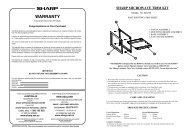
Replacement Procedure 

1. Turn the power off by pressing @F. 

2. Remove the two screws. (Fig. 1) 

3. Slide the battery cover slightly and lift it to remove. 

4. Remove the used batteries by prying them out with a ball-point 

pen or other similar pointed device. (Fig. 2) 

5. Install two new batteries. Make sure the “+” side is facing up. 

6. Replace the cover and screws. 

7. Press the RESET switch (on the back). 

• Make sure that the display appears as shown below. If the 

display does not appear as shown, remove the batteries, reinstall 

them and check the display once again. 

(Fig. 1) (Fig. 2) 

Automatic Power Off Function 

This calculator will turn itself off to save battery power if no key is 

pressed for approximately 10 minutes. 

SPECIFICATIONS 

Calculations: Scientific calculations, complex number 

calculations, equation solvers, statistical 

calculations, etc. 

Internal calculations: Mantissas of up to 14 digits 

Pending operations: 24 calculations 10 numeric values in the 

normal mode (5 numeric values in other 

modes, and 1 numeric value for Matrix/ 

List data.) 

Power source: Built-in solar cells 

3 V (DC): 

Backup batteries 

(Alkaline batteries (LR44 or equivalent) × 2) 

Operating temperature: 0°C – 40°C (32°F – 104°F) 

External dimensions: 79.6 mm (W) × 154.5 mm (D) × 13.2 mm (H) 

3-1/8” (W) × 6-3/32” (D) × 17/32” (H) 

Weight: Approx. 97g (0.22 lb) 

(Including batteries) 

Accessories: Batteries × 2 (installed), operation manual, 

quick reference card and hard case 

FOR MORE INFORMATION ABOUT 

SCIENTIFIC CALCULATOR 

Visit our Web site. 

http://sharp-world.com/calculator/ 

SHARP CORPORATION



CALCULATION EXAMPLES 

ANWENDUNGSBEISPIELE 

EXEMPLES DE CALCUL 

EJEMPLOS DE CÁLCULO 

EXEMPLOS DE CÁLCULO 

ESEMPI DI CALCOLO 

REKENVOORBEELDEN 

PÉLDASZÁMÍTÁSOK 

PŘÍKLADY VÝPOČTŮ 

RÄKNEEXEMPEL 

LASKENTAESIMERKKEJÄ 

èêàåÖêõ ÇõóàëãÖçàâ 

UDREGNINGSEKSEMPLER 

CONTOH-CONTOH PENGHITUNGAN 

CONTOH-CONTOH PERHITUNGAN 

CAÙC VÍ DUÏ PHEÙP TÍNH 

[] 

13(5+2)= ª 3 ( 5 + 2 )= 21. 

23×5+2= 3 * 5 + 2 = 17. 

33×5+3×2= 3 * 5 + 3 * 2 = 21. 

→1 @[ 21. 

→2 ] 17. 

→3 ] 21. 

→2 [ 17. 

” 

100000÷3= 

[NORM1] ª 100000 / 3 = 33’333.33333 

→[FIX] ”10 33’333.33333 

[TAB 2] ”2 2 33’333.33 

→[SCI] ”11 3.33 ×10 04– 

→[ENG] ”12 33.33 ×10 03– 

→[NORM1] ”13 33’333.33333 

3÷1000= 

[NORM1] ª 3 / 1000 = 0.003 

→[NORM2] ”14 3. ×10 –03 

→[NORM1] ”13 0.003 

+-*/()±E 

45+285÷3= ª 45 + 285 / 3 = 140. 

18+6 ( 18 + 6 )/ 

= 

15–8 ( 15 - 8 = 3.428571429 

42×(–5)+120= 42 *± 5 + 120 = –90. 

* 1 (5 ±) * 1 

(5×10 3 )÷(4×10 –3 )= 5 E 3 / 4 E 

± 3 = 1’250’000. 

34+57= 34 + 57 = 91. 

45+57= 45 + 57 = 102. 

68×25= 68 * 25 = 1’700. 

68×40= 68 * 40 = 2’720. 

sutSUTVhH 

Ile¡•L÷⁄ 

$#!qQ% 

sin60[°]= ªs 60 = 0.866025403 

π 

cos — [rad]= 

4 

”01u( 

@V/ 4 )= 0.707106781 

tan –11=[g] ”02@T 1 = 

”00 

50. 

(cosh 1.5 + ª(hu 1.5 +h 

sinh 1.5) 2 = s 1.5 )L= 20.08553692 

• • • • 

ENGLISH 

tanh –1 • • • • 

5 

— = 

7 

@Ht( 5 

/ 7 )= 0.895879734 

ln 20 = I 20 = 2.995732274 

log 50 = l 50 = 1.698970004 

e 3 = @e 3 = 20.08553692 

10 1.7 = @¡ 1.7 = 50.11872336 

1 1 

— + — = 

6 7 

6 @•+ 7 @ 

•= 0.309523809 

8 –2 – 3 4 × 5 2 = 8 ± 2 - 3 

4 * 5 L= –2’024.984375 

(123 ) — 4 = 

12 3 4 

@•= 6.447419591 

8 3 = 8 ÷= 512. 

¿49 – 4 ¿81 = @⁄ 49 - 4 @$ 

81 = 4. 

3 ¿27 = @# 27 = 3. 

4! = 4 @!= 24. 

10P 3 = 10 @q 3 = 720. 

5C 2 = 5 @Q 2 = 10. 

500×25%= 500 * 25 @% 125. 

120÷400=?% 120 / 400 @% 30. 

500+(500×25%)= 500 + 25 @% 625. 

400–(400×30%)= 400 - 30 @% 280. 

• 

• 

• 

• 

• 

• 

• 

• 

• 

• 

• 

• 

• 

• 

• 

• 

• 

• 

• 

1 

θ = sin –1 x, θ = tan –1 x θ = cos –1 x 

DEG –90 ≤ θ ≤ 90 0 ≤ θ ≤ 180 

RAD 

π π 

– — ≤ θ ≤ — 

2 2 

0 ≤ θ ≤ π 

GRAD –100 ≤ θ ≤ 100 0 ≤ θ ≤ 200 

Åè 

d/dx (x4 – 0.5x3 + 6x2 ) ªKˆ 4 - 0.5 K 

⎛ x=2 

⎜ 

⎝ dx=0.00002 

ˆ÷+ 6 KˆL 

@Å 2 ®® 50. 

⎛ x=3 

⎜ 

⎝ dx=0.001 

® 3 ® 0.001 ® 130.5000029 

∫ 8 

2 (x 2 – 5)dx ªKˆL- 5 

n=100 è 2 ® 8 ®® 138. 

n=10 ®®® 10 ® 138. 

g 

90°→ [rad] ª 90 @g 1.570796327 

→ [g] @g 100. 

→ [°] @g 90. 

sin –1 0.8 = [°] @S 0.8 = 53.13010235 

→ [rad] @g 0.927295218 

→ [g] @g 59.03344706 

→ [°] @g 53.13010235 

KRO;:?≥∆˚¬ 

ª 8 * 2 OM 16. 

24÷(8×2)= 24 /KM= 1.5 

(8×2)×5= KM* 5 = 80. 

ªOM 0. 

$150×3:M1 150 * 3 ; 450. 

+)$250:M2 =M1+250 250 ; 250. 

–)M2×5% RM* 5 @% 35. 

M @:RM 665. 

$1=¥110 110 OY 110. 

¥26,510=$? 26510 /RY= 241. 

$2,750=¥? 2750 *RY= 302’500. 

r=3cm (r→Y) 3 OY 3. 

πr 2 =? @VKYL= 28.27433388 

24 

—— = 2.4...(A) 24 /( 4 + 6 )= 2.4 

4+6 

3 *K?+ 60 / 

3×(A)+60÷(A)= 

K?= 32.2 

πr2⇒F1 @VKYL 

O≥ F1 

4 

3 OY 3. 

3 V = ? R≥* 4 / 3 = 37.69911184 

6+4=ANS ª 6 + 4 = 10. 

ANS+5 + 5 = 15. 

8×2=ANS 8 * 2 = 16. 

ANS 2 L= 256. 

44+37=ANS 44 + 37 = 81. 

√ANS= @⁄= 9. 

\| 

1 4 

3— + — = [a—] 

b 

2 3 c 

ª 3 \ 1 \ 2 + 

4 \ 3 = 4 l5 l6 * 

→[a.xxx] \ 4.833333333 

→[d/c] @| 29 l6 

10 — 2 

3 = @¡ 2 \ 3 = 4.641588834 

(—) 5 7 

5 

(—) — 

1 

1 3 

8 

= 7 \ 5 5 = 16807 l3125 

= 

1 \ 8 1 \ 3 

= 1 l2 

—— 

64 

= @⁄ 64 \ 225 = 8 l15 

225 

23 ( 2 3 ) \ 

34 — = 

( 3 4 ) = 8 l81 

1.2 

—– = 

2.3 

1°2’3” 

——– = 

2 

1×103 2×103 ——– = 

1.2 \ 2.3 = 12 l23 

1 o 2 o 3 \ 2 = 0°31’1.5” 

1 E 3 \ 2 E 3 = 1 l2 

A = 7 ª 7 OA 7. 

— 

4 

= 

A 

4 \KA= 4 l7 

1.25 + — 

2 

= [a.xxx] 

→[a—] 

b 

5 

c 

5 

* 4 l5 l6 = 4— 

6 

1.25 + 2 \ 5 = 

\ 

1.65 

1 l13 l20 

êûîìíãâ†ä 

àá 

DEC(25)→BIN ª@í 25 @ê 11001. b 

HEX(1AC) @ì 1AC 

→BIN @ê 110101100. b 

→PEN @û 3203. P 

→OCT @î 654. 0 

→DEC @í 428. 

BIN(1010–100) @ê( 1010 - 100 ) 

×11 = * 11 = 10010. b 

BIN(111)→NEG ã 111 = 1111111001. b 

HEX(1FF)+ @ì 1FF @î+ 

OCT(512)= 512 = 1511. 0 

HEX(?) @ì 349. H 

2FEC– ªOM@ì 2FEC - 

2C9E=(A) 2C9E ; 34E. H 

+)2000– 2000 - 

1901=(B) 1901 ; 6FF. H 

(C) RM A4d. H 

• • • •

• • • • 

1011 AND ª@ê 1011 † 

101 = (BIN) 101 = 1. b 

5A OR C3 = (HEX) @ì 5A ä C3 = db. H 

NOT 10110 = @êâ 10110 = 1111101001. b 

(BIN) 

24 XOR 4 = (OCT) @î 24 à 4 = 20. 0 

B3 XNOR @ì B3 á 

2D = (HEX) 2D = FFFFFFFF61. H 

→DEC @í –159. 

o_° (→sec, →min) 

12°39’18.05” ª 12 o 39 o 18.05 

→[10] @_ 12.65501389 

123.678→[60] 123.678 @_ 123°40’40.8” 

3h30m45s + 3 o 30 o 45 + 6 o 

6h45m36s = [60] 45 o 36 = 10°16’21.” 

1234°56’12” + 1234 o 56 o 12 + 

0°0’34.567” = [60] 0 o 0 o 34.567 = 1234°56’47.” 

3h45m – 3 o 45 - 1.69 = 

1.69h = [60] @_ 2°3’36.” 

sin62°12’24” = [10] s 62 o 12 o 24= 0.884635235 

24°→[”] 24 o°2 86’400. 

1500”→[ ’] 0 o 0 o 1500 °3 25. 

{},≠ 

⎛ x = 6 ⎛ r = 

⎜ → ⎜ 

⎝ y = 4 ⎝ θ = [°] 

ª 6 @, 4 

@{[r] 

@≠[θ] 

7.211102551 

33.69006753 

@≠[r] 7.211102551 

⎛ r = 14 ⎛ x = 

⎜ → ⎜ 

⎝ θ = 36[°] ⎝ y = 

14 @, 36 

@}[x] 

@≠[y] 

11.32623792 

8.228993532 

@≠[x] 11.32623792 

ß 

V0 = 15.3m/s ª 15.3 * 10 + 2 @•* 

t = 10s 

1 2 V0t+ — gt = ?m 

2 

ß 03 * 10 L= 643.3325 

¥ 

125yd = ?m ª 125 @¥ 5 = 114.3 

∑ (k, M, G, T, m, Ì, n, p, f) 

100m×10k= 100 ∑14* 

10 ∑10= 1’000. 

j” 

5÷9=ANS ª”10”2 1 

ANS×9= 5 / 9 = 0.6 

[FIX,TAB=1] * 9 =* 1 5.0 

5 / 9 =@j 0.6 

* 9 =* 2 5.4 

”13 

* 1 5.5555555555555×10 –1 ×9 

* 2 0.6×9 

∑ (SOLV) 

sin x–0.5 ªsKˆ- 0.5 

Start= 0 ∑0 0 ®® 30. 

Start= 180 ® 180 ®® 150. 

≤ 

m0 

f(x) = x 3 –3x 2 +2 Kˆ 3 - 3 K 

ˆL+ 2 @≤ 

x = –1 1 ±® –2. 

x = –0.5 @≤ 0.5 ±® 1.125 

A 2 +B 2 @⁄(KAL+ 

KBL)@≤ 

A = 2, B = 3 2 ® 3 ® 3.605551275 

A = 2, B = 5 @≤® 5 ® 5.385164807 

k&~£pnzw^ 

¢PZWvrab© 

xy≠° (→t, P(, Q(, R() 

DATA 

95 m10 0. 

80 95 k 1. 

80 80 k 2. 

75 k 3. 

75 75 & 3 k 4. 

75 50 k 5. 

50 

–x= R~ 75.71428571 

σx= Rp 12.37179148 

n= Rn 7. 

Σx= Rz 530. 

Σx 2 = Rw 41’200. 

sx= R£ 13.3630621 

sx 2 = L= 178.5714286 

(95– – x) 

sx 

×10+50= 

( 95 -K~) 

/K£* 10 

+ 50 = 64.43210706 

x = 60 → P(t) ? °1 60 °0)= 0.102012 

t = –0.5 → R(t) ? °3 0.5 ±)= 0.691463 

x y m11 0. 

2 5 2 & 5 k 1. 

2 5 k 2. 

12 24 12 & 24 k 3. 

21 40 21 & 40 & 3 k 4. 

21 40 15 & 25 k 5. 

21 40 Ra 1.050261097 

15 25 Rb 1.826044386 

Rr 0.995176343 

R£ 8.541216597 

R¢ 15.67223812 

x=3 → y′=? 3 @y 6.528394256 

y=46 → x′=? 46 @x 24.61590706 

x y m12 0. 

12 41 12 & 41 k 1. 

8 13 8 & 13 k 2. 

5 2 5 & 2 k 3. 

23 200 23 & 200 k 4. 

15 71 15 & 71 k 5. 

Ra 5.357506761 

Rb –3.120289663 

R© 0.503334057 

x=10 → y′=? 10 @y 24.4880159 

y=22 → x′=? 22 @x 9.63201409 

@≠ –3.432772026 

@≠ 9.63201409 

k[] 

DATA 

30 m10 0. 

40 30 k 1. 

40 40 & 2 k 2. 

50 50 k 3. 

↓ 

DATA 

30 ]]] 

45 45 & 3 k X2= 45. 

45 ] N2= 3. 

45 

60 ] 60 k X3= 60. 

x = Σx 

n 

sx = Σx2 – nx2 

n – 1 

y = Σy 

n 

sy = Σy2 – ny2 

n – 1 

σx = Σx2 – nx2 

n 

Σx = x1 + x2 + ··· + xn 

Σx 2 = x1 2 + x2 2 + ··· + xn 2 

σy = Σy2 – ny2 

n 

Σxy = x1y1 + x2y2 + ··· + xnyn 

Σy = y1 + y2 + ··· + yn 

Σy 2 = y1 2 + y2 2 + ··· + yn 2

t = –––– x – x 

σx 

Standardization conversion formula 

Standard Umrechnungsformel 

Formule de conversion de standardisation 

Fórmula de conversión de estandarización 

Fórmula de conversão padronizada 

Formula di conversione della standardizzazione 

Standaardisering omzettingsformule 

Standard átváltási képlet 

Vzorec pro přepočet rozdělení 

Omvandlingsformel för standardisering 

Normituksen konversiokaava 

îÓappleÏÛÎ‡ ÒÚ‡Ì‰‡appleÚËÁÓ‚‡ÌÌÓ„Ó ÔappleÂÓ·apple‡ÁÓ‚‡ÌËfl 

Omregningsformel for standardisering 

Rumus penukaran pemiawaian 

Rumus konversi standarisasi 

Coâng thöùc bieán ñoåi chuaån hoùa 

m (2-VLE) 

a1x + b1y = c1 a2x + b2y = c2 

⎧2x 

+ 3y = 4 

⎨ 

⎩5x 

+ 6y = 7 

m20 

2 ® 3 ® 4 ® 

5 ® 6 ® 7 

x = ? ® [x] –1. 

y = ? ® [y] 2. 

det(D) = ? ® [det(D)] –3. 

m (3-VLE) 

a1x + b1y + c1z = d1 a2x + b2y + c2z = d2 

a3x + b3y + c3z = d3 

⎧ x + y – z = 9 

m21 

1 ® 1 ® 1 ±® 9 ® 

⎨ 6x + 6y – z = 17 

⎩14x 

– 7y + 2z = 42 

6 ® 6 ® 1 ±® 17 ® 

14 ® 7 ±® 2 ® 42 

x = ? ® [x] 3.238095238 

y = ? ® [y] –1.638095238 

z = ? ® [z] –7.4 

det(D) = ? ® [det(D)] 105. 

m (QUAD, CUBIC) 

m22 

3x 2 + 4x – 95 = 0 3 ® 4 ®± 95 

x1 = ? ® 5. 

x2 = ? ® –6.333333333 

@® 5. 

5x 

m23 

3 +4x2 +3x +7=0 5 ® 4 ® 3 ® 7 

x1 = ? ® –1.233600307 i 

x2 = ? ® 0.216800153 i 

@≠ 

+ 1.043018296 i 

x3 = ? ® 0.216800153 i 

@≠ 

– 1.043018296 i 

m (CPLX) 

(12–6i) + (7+15i) – 

m3 

12 - 6 Ü+ 7 + 15 Ü- 

(11+4i) = ( 11 + 4 Ü)= [x] 8. i 

@≠ [y] 

+ 5. i 

@≠ [x] 8. i 

6×(7–9i) × 6 *( 7 - 9 Ü)* 

(–5+8i) = ( 5 ±+ 8 Ü)= [x] 222. i 

@≠ [y] 

+ 606. i 

16×(sin30°+ 16 *(s 30 + 

icos30°)÷(sin60°+ Üu 30 )/(s 60 + 

icos60°)= Üu 60 )= [x] 13.85640646 i 

@≠ [y] 

+ 8. i 

• • • • 

D = 

D = 

a 1 b 1 

a 2 b2 

a 1 b 1 c 1 

a 2 b2 c2 

a 3 b3 c3 

y • • • • 

@{ 8 Ö 70 + 12 Ö 25 

• • • • 

stdDv L1 = 2.516611478 ª∑46∑00= 

A 

r1 

θ1 

r 

θ B 

r2 

θ2 

= [r] 

@≠ [θ] 

18.5408873 i 

∠ 42.76427608 i 

vari L1 = 6.333333333 ª∑47∑00= 

x 

r1 = 8, θ1 = 70° 

r2 = 12, θ2 = 25° 

↓ 

r = ?, θ = ?° 

(1 + i) @} 1 +Ü= 1. i 

↓ @{ [r] 1.414213562 i 

r = ?, θ = ?° @≠ [θ] ∠ 45. i 

(2 – 3i) 

@}( 2 - 3 Ü)L 

2 = = [x] –5. i 

@≠ [y] 

– 12. i 

1 ( 1 +Ü)@•= [x] 0.5 i 

—— = 

1 + i @≠ [y] – 0.5 i 

CONJ(5+2i) = ∑0( 5 + 2 Ü)= [x] 5. i 

@≠ [y] 

– 2. i 

m (MAT) 

m4 

1 2 ] 2 k 2 k 1 k 2 k 

→ matA 

3 4 3 k 4 k 

ª∑20 

3 1 

→ matB 

] 2 k 2 k 

2 6 

3 k 1 k 2 k 6 k 

ª∑21 

matA × matB = 7 13 17 27 

ª∑00*∑01= 

matA –1 = 

–2 1 

1.5 –0.5 

ª∑00@•= 

dim(matA,3,3) = 1 2 0 

dim(matA,3,3) = 3 4 0 

dim(matA,3,3) = 0 0 0 

ª∑30∑00 

@, 3 @, 3 )= 

fill(5,3,3) = 5 5 5 

fill(5,3,3) = 5 5 5 

fill(5,3,3) = 5 5 5 

ª∑31 5 @, 

3 @, 3 )= 

cumul matA = 

1 2 

4 6 

ª∑32∑00= 

aug(matA,matB) = 

identity 3 = 1 0 0 

1 2 3 1 

3 4 2 6 

ª∑33∑00 

@,∑01)= 



ª∑34 3 = 

rnd_mat(2,3) ª∑35 2 @, 3 )= 

det matA = –2 ª∑40∑00= 

trans matB = 

3 2 

1 6 

mat → list L1: {1 3} ª∑5 

L2: {3 2} 

m (LIST) 

ª∑41∑01= 

m5 

2, 7, 4 → L1 ] 3 k 2 k 7 k 4 k 

ª∑20 

–3, –1, –4 → L2 

] 3 k 

± 3 k± 1 k± 4 k 

ª∑21 

L1+L2 = {–1 6 0} ª∑00+∑01= 

sortA L1 = {2 4 7} ª∑30∑00= 

sortD L1 = {7 4 2} ª∑31∑00= 

dim(L1,5) = {2 7 4 0 0} 

fill(5,5) = {5 5 5 5 5} 

ª∑32∑00 

@, 5 )= 

ª∑33 5 @, 

5 )= 

cumul L1 = {2 9 13} ª∑34∑00= 

df_list L1 = {5 –3} ª∑35∑00= 

aug(L1,L2) = {2 7 4 –3 –1 –4} ª∑36∑00 

@,∑01)= 

min L1 = 2 ª∑40∑00= 

max L1 = 7 ª∑41∑00= 

mean L1 = 4.333333333 ª∑42∑00= 

med L1 = 4 ª∑43∑00= 

sum L1 = 13 ª∑44∑00= 

prod L1 = 56 ª∑45∑00= 

• • • • 

o_prod(L1,L2) = {–24 –4 19} ª∑48∑00 

@,∑01)= 

i_prod(L1,L2) = –29 ª∑49∑00 

@,∑01)= 

abs L2 = 5.099019514 ª∑4A∑01= 

list → matA matA: 2 –3 

list → matA matA: 7 –1 ª∑6 

list → matA matA: 4 –4 

Function Dynamic range 

Funktion zulässiger Bereich 

Fonction Plage dynamique 

Función Rango dinámico 

Função Gama dinâmica 

Funzioni Campi dinamici 

Functie Rekencapaciteit 

Függvény Megengedett számítási tartomány 

Funkce Dynamický rozsah 

Funktion Definitionsområde 

Funktio Dynaaminen ala 

îÛÌÍˆËfl ÑËÌ‡ÏË˜ÂÒÍËÈ ‰Ë‡Ô‡ÁÓÌ 

Funktion Dynamikområde 

Fungsi Julat dinamik 

Fungsi Kisaran dinamis 

Haøm soá Giôùi haïn Ñoäng 

DEG: | x | < 10 10 

(tan x : | x | ≠ 90 (2n–1))* 

sin x, cos x, RAD: | x | < —– × 10 10 

tan x 

GRAD: 

(tan x : | x | ≠ — (2n–1))* 

| x | < —– × 10 10 

π 

180 

π 

2 

10 

9 

(tan x : | x | ≠ 100 (2n–1))* 

sin –1x, cos –1x | x | ≤ 1 

tan –1x, 3 ¿x | x | < 10100 In x, log x 10 –99 ≤ x < 10100 

• y > 0: –10100 < x log y < 100 

• y = 0: 0 < x < 10100 yx • y < 0: x = n 

(0 < l x l < 1: — = 2n–1, x ≠ 0)*, 

–10100 < x log | y | < 100 

• y > 0: –10100 < — log y < 100 (x ≠ 0) 

• y = 0: 0 < x < 10100 x ¿y • y < 0: x = 2n–1 

(0 < | x | < 1 : — = n, x ≠ 0)*, 

–10100 1 

x 

1 

x 

1 

1 

x 

< — log | y | < 100 

x 

ex –10100 < x ≤ 230.2585092 

10x –10100 < x < 100 

sinh x, cosh x, 

tanh x 

| x | ≤ 230.2585092 

sinh –1 x | x | < 1050 cosh –1 x 1 ≤ x < 1050 tanh –1 x | x | < 1 

x2 | x | < 1050 x3 | x | < 2.15443469 × 1033 ¿x 0 ≤ x < 10100 x –1 | x | < 10100 (x ≠ 0) 

n! 0 ≤ n ≤ 69* 

0 ≤ r ≤ n ≤ 9999999999* 

nPr 

—— < 10100 n! 

(n-r)! 

nCr 

0 ≤ r ≤ n ≤ 9999999999* 

0 ≤ r ≤ 69 

—— < 10100 n! 

(n-r)! 

↔DEG, D°M’S 0°0’0.00001” ≤ | x | < 10000° 

x, y → r, θ x2 + y2 < 10100 0 ≤ r < 10100 DEG: | θ | < 10 10 

r, θ → x, y RAD: | θ | < —– × 10 10 

GRAD : | θ | < — × 10 10 

π 

180 

10 

9 

DEG→RAD, GRAD→DEG: | x | < 10100 DRG | 

RAD→GRAD: | x | < — × 1098 (A+Bi)+(C+Di) | A + C | < 10100 , | B + D | < 10100 π 

2 

(A+Bi)–(C+Di) | A – C | < 10 100 , | B – D | < 10 100 

(A+Bi)×(C+Di) 

• • • • 

(AC – BD) < 10 100 

(AD + BC) < 10 100

• • • • Endast svensk version/For Sweden only: 

In Europe: 

AC + BD < 10 100 

C 2 + D 2 

(A+Bi)÷(C+Di) BC – AD 100 < 10 

C2 + D2 C2 + D2 ≠ 0 

→DEC DEC : | x | ≤ 9999999999 

→BIN BIN : 1000000000 ≤ x ≤ 1111111111 

→PEN 0 ≤ x ≤ 111111111 

→OCT PEN : 2222222223 ≤ x ≤ 4444444444 

→HEX 0 ≤ x ≤ 2222222222 

AND OCT : 4000000000 ≤ x ≤ 7777777777 

OR 0 ≤ x ≤ 3777777777 

XOR HEX : FDABF41C01 ≤ x ≤ FFFFFFFFFF 

XNOR 0 ≤ x ≤ 2540BE3FF 

BIN : 1000000000 ≤ x ≤ 1111111111 

0 ≤ x ≤ 111111111 

PEN : 2222222223 ≤ x ≤ 4444444444 

NOT 

OCT 

0 ≤ x ≤ 2222222221 

: 4000000000 ≤ x ≤ 7777777777 

0 ≤ x ≤ 3777777777 

HEX : FDABF41C01 ≤ x ≤ FFFFFFFFFF 

0 ≤ x ≤ 2540BE3FE 

BIN : 1000000001 ≤ x ≤ 1111111111 

0 ≤ x ≤ 111111111 

PEN : 2222222223 ≤ x ≤ 4444444444 

NEG 

OCT 

0 ≤ x ≤ 2222222222 

: 4000000001 ≤ x ≤ 7777777777 

0 ≤ x ≤ 3777777777 

HEX : FDABF41C01 ≤ x ≤ FFFFFFFFFF 

0 ≤ x ≤ 2540BE3FF 

* n, r: integer / ganze Zahlen / entier / entero / inteiro / intero / 

geheel getal / egész számok / celé číslo / heltal / 

kokonaisluku / ˆÂÎ˚Â / heltal / / / / 

integer / bilangan bulat / soá nguyeân 

This equipment complies with the requirements of Directive 89/336/ 

EEC as amended by 93/68/EEC. 

Dieses Gerät entspricht den Anforderungen der EG-Richtlinie 89/336/ 

EWG mit Änderung 93/68/EWG. 

Ce matériel répond aux exigences contenues dans la directive 89/336/ 

CEE modifiée par la directive 93/68/CEE. 

Dit apparaat voldoet aan de eisen van de richtlijn 89/336/EEG, 

gewijzigd door 93/68/EEG. 

Dette udstyr overholder kravene i direktiv nr. 89/336/EEC med tillæg 

nr. 93/68/EEC. 

Quest’ apparecchio è conforme ai requisiti della direttiva 89/336/EEC 

come emendata dalla direttiva 93/68/EEC. 

 

89/336/, 

93/68/. 

Este equipamento obedece às exigências da directiva 89/336/CEE na 

sua versão corrigida pela directiva 93/68/CEE. 

Este aparato satisface las exigencias de la Directiva 89/336/CEE 

modificada por medio de la 93/68/CEE. 

Denna utrustning uppfyller kraven enligt riktlinjen 89/336/EEC så som 

kompletteras av 93/68/EEC. 

Dette produktet oppfyller betingelsene i direktivet 89/336/EEC i 

endringen 93/68/EEC. 

Tämä laite täyttää direktiivin 89/336/EEC vaatimukset, jota on 

muutettu direktiivillä 93/68/EEC. 

Ñ‡ÌÌÓÂ ÛÒÚappleÓÈÒÚ‚Ó ÒÓÓÚ‚ÂÚÒÚ‚ÛÂÚ ÚappleÂ·Ó‚‡ÌËflÏ ‰ËappleÂÍÚË‚˚ 89/336/ 

EEC Ò Û˜ÂÚÓÏ ÔÓÔapple‡‚ÓÍ 93/68/EEC. 

Ez a készülék megfelel a 89/336/EGK sz. EK-irányelvben és annak 93/ 

68/EGK sz. módosításában foglalt követelményeknek. 

Tento pfiístroj vyhovuje poÏadavkÛm smûrnice 89/336/EEC v platném 

znûní 93/68/EEC. 

Nur für Deutschland/For Germany only: 

Umweltschutz 

Das Gerät wird durch eine Batterie mit Strom versorgt. 

Um die Batterie sicher und umweltschonend zu entsorgen, 

beachten Sie bitte folgende Punkte: 

• Bringen Sie die leere Batterie zu Ihrer örtlichen Mülldeponie, 

zum Händler oder zum Kundenservice-Zentrum zur 

Wiederverwertung. 

• Werfen Sie die leere Batterie niemals ins Feuer, ins Wasser 

oder in den Hausmüll. 

Seulement pour la France/For France only: 

Protection de l’environnement 

L’appareil est alimenté par pile. Afin de protéger 

l’environnement, nous vous recommandons: 

• d’apporter la pile usagée ou à votre revendeur ou au service 

après-vente, pour recyclage. 

• de ne pas jeter la pile usagée dans une source de chaleur, 

dans l’eau ou dans un vide-ordures. 

Miljöskydd 

Denna produkt drivs av batteri. 

Vid batteribyte skall följande iakttagas: 

• Det förbrukade batteriet skall inlämnas till er lokala handlare 

eller till kommunal miljöstation för återinssamling. 

• Kasta ej batteriet i vattnet eller i hushållssoporna. Batteriet 

får ej heller utsättas för öppen eld. 

OPMERKING: ALLEEN VOOR NEDERLAND/ 

NOTE: FOR NETHERLANDS ONLY 

• Physical Constants and Metric Conversions are shown in the 

tables. 

• Physikalischen Konstanten und metriche Umrechnungen sind 

in der Tabelle aufgelistet. 

• Les constants physiques et les conversion des unités sont 

indiquées sur les tableaux. 

• Las constants fisicas y conversiones métricas son mostradas 

en las tables. 

• Constantes Fisicas e Conversões Métricas estão mostradas 

nas tablelas. 

• La constanti fisiche e le conversioni delle unità di misura 

vengono mostrate nella tabella. 

• De natuurconstanten en metrische omrekeningen staan in de 

tabellen hiernaast. 

• A fizikai konstansok és a metrikus átváltások a táblázatokban 

találhatók. 

• Fyzikální konstanty a převody do metrické soustavy jsou 

uvedeny v tabulce. 

• Fysikaliska konstanter och metriska omvandlingar visas i 

tabellerna. 

• Fysikaaliset vakiot ja metrimuunnokset näkyvät taulukoista. 

• Ç Ú‡·ÎËˆ‡ı ÔÓÍ‡Á‡Ì˚ ÙËÁË˜ÂÒÍËÂ ÍÓÌÒÚ‡ÌÚ˚ Ë 

ÏÂÚappleË˜ÂÒÍËÂ ÔappleÂÓ·apple‡ÁÓ‚‡ÌËfl. 

• Fysiske konstanter og metriske omskrivninger vises i tabellen. 

• 

• 

• 

• Pemalar Fizik dan Pertukaran Metrik ditunjukkan di dalam 

jadual. 

• Konstanta Fisika dan Konversi Metrik diperlihatkan di dalam 

tabel. 

• Caùc Haèng soá Vaät lyù vaø caùc Pheùp bieán ñoåi Heä meùt ñöôïc theå 

hieän trong caùc baûng. 

PHYSICAL CONSTANTS ß 01 — 52 

No. SYMBOL UNIT No. SYMBOL UNIT No. SYMBOL UNIT 

01 - c, c 0 m s –1 19 - µΒ J T –1 37 - eV J 

02 - G m 3 kg –1 s –2 20 - µe J T –1 38 - t K 

03 - gn m s –2 21 - µΝ J T –1 39 - AU m 

04 - me kg 22 - µp J T –1 40 - pc m 

05 - mp kg 23 - µn J T –1 41 - M( 12 C) kg mol –1 

06 - mn kg 24 - µµ J T –1 42 - h - J s 

07 - mµ kg 25 - λc m 43 - Eh J 

08 - lu kg 26 - λc, p m 44 - G 0 s 

09 - e C 27 - σ W m –2 K –4 45 - α –1 

10 - h J s 28 - NΑ, L mol –1 46 - mp/me 

11 - k J K –1 29 - Vm m 3 mol –1 47 - Mu kg mol –1 

12 - µ 0 N A –2 30 - R J mol –1 K –1 48 - λc, n m 

13 - ε0 F m –1 31 - F C mol –1 49 - c 1 W m 2 

14 - re m 32 - R K Ohm 50 - c2 m K 

15 - α 33 - -e/me C kg –1 51 - Z 0 Ω 

16 - a 0 m 34 - h/2me m 2 s –1 52 - Pa 

17 - R∞ m –1 35 - γp s –1 T –1 

18 - Φ 0 Wb 36 - KJ Hz V –1 

METRIC CONVERSIONS x @¥ 1 — 44 

No. UNIT No. UNIT No. UNIT 

1 in→cm 16 kg→lb 31 J→calIT 

2 cm→in 17 °F→°C 32 calIT→J 

3 ft→m 18 °C→°F 33 hp→W 

4 m→ft 19 gal (US)→l 34 W→hp 

5 yd→m 20 l→gal (US) 35 ps→W 

6 m→yd 21 gal (UK)→l 36 W→ps 

7 mile→km 22 l→gal (UK) 37 kgf/cm 2 →Pa 

8 km→mile 23 fl oz (US)→ml 38 Pa→kgf/cm 2 

9 n mile→m 24 ml→fl oz (US) 39 atm→Pa 

10 m→n mile 25 fl oz (UK)→ml 40 Pa→atm 

11 acre→m 2 26 ml→fl oz (UK) 41 mmHg→Pa 

12 m 2 →acre 27 J→cal 42 Pa→mmHg 

13 oz→g 28 cal→J 43 kgf·m→J 

14 g→oz 29 J→cal15 44 J→kgf·m 

15 lb→kg 30 cal15→J

EL-506W EL-546W - Sharp Australia Support

Create successful ePaper yourself

Delete template?

Save as template?