Homework Set Four ECE 175 Department of ... - UCSD DSP Lab

Homework Set Four
ECE 175
Department of Electrical and Computer Engineering
University of California, San Diego
N. Vasconcelos & K. Kreutz-Delgado Winter 2011
Due Thursday, March 3, 2011
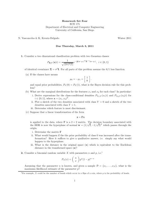
1. Consider a two dimensional classification problem with two Gaussian classes
P X|Y (x|i) =
1
1 − e 2
(2π) 2 |Σ| (x−µi)T Σ −1 (x−µi)
, i ∈{0, 1}
of identical covariance Σ = σ 2 I. For all parts of this problem assume the 0/1 loss function.
(a) If the classes have means
μ0 = −μ1 =
and equal prior probabilities, PY (0) = PY (1), what is the Bayes decision rule for this problem?
(b) What are the marginal distributions for the features x1 and x2 for each class? In particular:
i. Derive expressions for the class-conditional densities PX1|Y (x1|i) andPX2|Y (x2|i) for
i ∈{0, 1}, wherex =(x1,x2) T .
ii. Plot a sketch of the two densities associated with class Y = 0 and a sketch of the two
densities associated with class Y =1.
iii. Determine which feature is most discriminant.
(c) Suppose that a linear transformation of the form
z = Γx
is applied to the data, where Γ is a 2 × 2 matrix. The decision boundary associated with
the BDR is now the hyperplane of normal w =(1/ √ 2, −1/ √ 2) T which passes through the
origin.
i. Determine the matrix Γ
ii. What would happen if the the prior probability of class 0 was increased after the transformation?
Here it suffices to give a qualitative answer, i.e. simply say what would
happen to the hyperplane.
iii. What is the distance in the original space (x) which is equivalent to the Euclidean
distance in the transformed space (z)?
1
0
2. Consider a binomial random variable X with parameters n and p, i.e. 1
PX(x) =
n
x
.
p x (1 − p) n−x
Assuming that the parameter n is known, and given a sample D = {x1,...,xN }, what is the
maximum likelihood estimate of the parameter p?
1 For example, X could be the number of heads which occur in n flips of a coin, where p is the probability of heads.
1

3. Consider an m-dimensional random vectors Y, such that 2
Y = Ax + N
where A is a full rank matrix and x is an unknown, but deterministic, n-dimensional vector, with
n

5. Continuation of Computer Assignment.
In the last two computer problems, we saw how classification of hand written digits works. This
time we will move to a more general and practical situation. For this problem, you are to use the
data-set given with Homework 4.
We shall continue with the same training data used in the previous computer experiments, but
with a new set of test data testImagesNew, which has been intentionally: 1) corrupted by noise
and 2) re-scaled (attenuated) in amplitude.
This corresponds to the situation where we have clean training data (which presumably has
been imaged using high-quality imaging systems in under optimal lighting), but poorer quality
test data corresponding to the type of run-time digits images that would be produced using
inexpensive image-scanners in poorly illuminated environments. (Poor illumination leads to contrast
attenuation, and pixel-noise if the scanner is low-quality.) The image on the left of Fig.1
shows the case of an intensity-attenuated, noisy digital scan of the digit on the left. We want to
classify such corrupted digits using a NN classifier.
We shall continue with the same training data used in the previous experiment, but with a new
setoftestdatatestImagesNew, which has been intentionally: 1) re-scaled in amplitude, and 2)
corrupted by noise.
Using the Nearest Neighbor approach, we will find the training image that is nearest to an estimate
of the uncorrupted test image. I.e., instead of the using the Euclidean distances between the
training images and the corrupted test image, we will use the Euclidean distances between the
training images and the ML estimate of the uncorrupted test image.
Toward this end, we assume that a corrupted test image Y is a random vector of the form
Y = a X + N
i.e. the result of corrupting an unknown clean image X through 1) amplitude re-scaling by
the scalar a, and 2) addition of independent zero mean Gaussian noise with variance v, i.e.
N ∼G(0,vI).
The approach to be used is:
(a) Determine a maximum likelihood estimate (MLE), âML, of the attenuation parameter a. The
simplest way to to this is if we are given given the corrupted observation y (the test image)
corresponding to a known training image x. 3 In which case we can compute the conditional
MLE of a, 4
âML =argmaxPY|X(y|x;
a, v) . (4)
a
(b) Given the test image y and the MLE of the parameter a, determine the maximum likelihood
estimate (MLE) ˆx ML of the unknown “clean image” x, assuming the model given in Eq. (4)
(but with a approximated by its maximum likelihood estimate). 5
(c) Determine the closest training image, x, toˆx ML. Once the closest training image has been
found, its label is assigned to the test image y, thereby performing a classification of y. (I.e.,
the Euclidean distance between the scaled test image, ˆx ML, and a training image, x, serves
asthemetricfortheNNclassifier.)
3This will be the case here. If this were not the case, the problem would be much harder and we would have to be
much cleverer on how to do this.
4What about the variance parameter v?
5Consistent with intuition, you should find that ˆxML is a scaled version of the test image y. I.e., you should find that
ˆxML = c y. What do you intuitively think the value of the scale parameter c should be?
3

Perform the following:
(i) Using the two sample images sampletest.png and sampletrain.png, calculate the maximum
likelihood estimate (MLE), â ML, of the scale parameter a in Eq. (4).
(ii) Using the MLE â ML in place of a in Eq. (4), determine a formula which expresses ˆx ML as a
function of y.
Figure 1: Sample Images: Corrupted on the left. Clean on the right.
(iii) Now for the new testset testImagesNew, perform the task of classification using the leastsquares
distance metric applied to ˆx ML (which is computed from y). As was done for our
previous computer assignments, compute and plot the error rates for each class, and the total
error rate.
(iv) Perform a NN classification on the new testset, using the simple algorithm of Computer
Problem 1, i.e. using Euclidean distance metric applied to y (instead of to ˆx ML, asdone
in the previous step). Compare your results with the NN classification performed in the
previous step.
Notes:
• Convert everything to double precision before calculating the MLE of a.
• All the data needed for this assignment is uploaded on the website. Do not use data
from the previous experiments.
4