X - UCSD DSP Lab

Some Linear Algebra Concepts
Ken Kreutz-Delgado
Nuno Vasconcelos
ECE 175A – Winter 2011 – UCSD

Vector spaces
• Definition: a vector space is a set H where
– addition and scalar multiplication are defined and satisfy:
1) x+(x’+x’’) = (x+x’)+x” 5) lx H
2) x+x’ = x’+x H 6) 1x = x
3) 0 H, 0 + x = x 7) l(l’ x) = (ll’)x
4) –x H, -x + x = 0 8) l(x+x’) = lx + lx’
(l=scalar) 9) (l+l’)x = lx + l’x
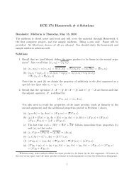
• the canonical example is d with standard
vector addition and scalar multiplication
e 2
e d
x
x’
x+x’
e 1
e 2
e d
x
ax
e 1

Vector spaces
• But there are much more interesting examples
• E.g., the space of functions f:X with
(f+g)(x) = f(x) + g(x) (lf)(x) = lf(x)
• d is a vector space of
finite dimension,e.g.
– f = (f 1, ..., f d)
• When d goes to infinity
we have a function
– f = f(t)
• The space of all functions
is an infinite dimensional
vector space

Data
• In this course we will talk a lot about “data”
• In all cases data will be represented in a vector space:
– an example is really just a point (“datapoint”) on such a space
– from above we know how to perform basic operations on
datapoints
– this is nice, because datapoints can be quite abstract
– e.g. images:
an image is a function
on the image plane
it assigns a color f(x,y) to
each each image
location (x,y)
the space Y of images
is a vector space (note: assumes
that images can be negative)
this image is a point in Y

Images
• Because of this we can manipulate images by
manipulating their equivalent vector representations
• E.g., Suppose one wants to “morph” a(x,y) into b(x,y):
– One way to do this is via the path along the line from a to b.
c(a) = a + a(b-a)
= (1-a) a + a b
– for a = 0 we have a
– for a = 1 we have b
– for a in (0,1) we have a point
on the line between a and b
• To morph an image we can simply
apply this rule to the image vector
representations!
b
b-a
a
a(b-a)

Images
• When we make
c(x,y) = (1-a) a(x,y) + a b(x,y)
we get “image morphing”:
a=0 a=0.2 a=0.4
a=0.6 a=0.8 a=1
• The point is that this is possible because we are in a
vector space.
b
b-a
a
a(b-a)

Images
• Images are approximately represented as points in d
– Sample (discretize) image on a finite grid to get array of pixels
a(x,y) a(i,j)
– Images are always stored like this on computers
– Stack all the rows into a vector, e.g. a 3 x 3 image is converted
into a 9 x 1 vector
– A n x m image vector is transformed into a nm x 1 vector
– Note that this is yet another vector space
• The point is that there are multiple isomorphic vector
spaces in which the data can be represented

Text
• Another common type
of data is text
• Documents are
represented by
word counts:
– associate a counter
with each word
– slide a window through
the text
– whenever the word
occurs increment
its counter
• This is the way search
engines represent
web pages

Text
• E.g. word counts for three
documents in a certain corpus
(only 12 words shown for clarity)
• Note that:
– Each document is a 12
dimensional vector
– If I add two word count vectors (documents), I get a new word
count vector (document)
– If I multiply a word count vector (document) by a scalar, I get a
word count vector
– Note: once again we assume word counts could be negative (to
make this happen we can simply subtract the average value)
• This means:
– We are once again on a vector space (positive subset of d )
– A document is a point in this space

Bilinear forms
• One reason to use vector spaces is that they allow us to
measure distances between data points
• We will see that this is crucial for classification
• The main tool for this is the inner product (dot-product).
• We can define the dot-product using the notion of a
bilinear form (assuming a real vector space).
• Definition: a bilinear form on a vector space H is a
bilinear mapping
Q: H x H
(x,x’) Q(x,x’)
“Bi-linear” means that "x,x’,x’’ H
i) Q[(lx+lx’),x”] = lQ(x,x”) + l’Q(x’,x”)
ii) Q[x”,(lx+lx’)] = lQ(x”,x) + l’Q(x”,x’)

Inner Products
• Definition: an inner product on a real vector space H
is a bilinear form
: H x H
(x,x’)
such that
i) 0, "x H
ii) = 0 if and only if x = 0
iii) = for all x and y
• The positive-definiteness conditions i) and ii) make the
inner product a natural measure of similarity
• This becomes more precise with introduction of a norm

Inner Products and Norms
• Any inner product induces a norm via the definition
||x|| 2 =
• By definition, any norm must obey the following properties
– Positive-definiteness: ||x|| 0, & ||x|| = 0 iff x =0
– Homogeneity: ||l x|| = |l| ||x||
– Triangle Inequality: ||x + y|| ≤ ||x|| + ||y||
• A norm defines a corresponding metric
d(x,y) = ||x-y||
which is a measure of the distance between x and y
• Always remember that the induced norm changes with a
different choice of inner product!

Inner Product
• Back to our examples:
– In d the standard (or unweighted) inner product is
d
T
x, y = x y =
i=
1
– Which leads to the standard Euclidean norm in d
x
=
x
T
x
=
– The distance between two vectors is the standard Euclidean
distance in d
d(
x,
y)
=
x y
=
x
i
d
i=
1
( x y)
T
y
x
i
2
i
( x y)
=
d
i=
1
( x
i
y
i
2
)

Inner Products and Norms
• Note that this immediately gives
a measure of similarity
between web pages
– compute word count vector x i
from page i, for all i
– distance between page i and
page j is simply
T
d( xi,
x j ) =
xi
x j = ( xi
x j ) ( xi
x j )
– this allows us to find, in the web, the most similar page i to any
given page j
• This is very close to the measure of similarity used by
most search engines!
• What about functions, e.g. on images?

Inner Products on Function Spaces
• Recall that the space of functions is an infinite
dimensional vector space
– The standard (unweighted) inner product is the natural
extension of that in d (just replace summations by integrals)
f ( x), g( x) = f ( x) g( x) dx
– the norm is related to the “energy” of the function
2 2
f ( x) = f ( x) dx
– and the distance between functions is related to the energy of
the difference between them
2 2
d( f ( x), g( x)) = f ( x) g( x) = [ f ( x) g( x)] dx

Basis
• We know how to measure distances in a vector space
• Another interesting property is that we can fully
characterize the space by one of its bases
• A set of vectors x 1, …, x k are a basis of a vector space H
if and only if (iff)
– they are linearly independent
i
c x = 0 c = 0,
" i
i
i
– And they span H : for any v in H, v can be written as
v
=
i
i i x c
• These two conditions mean that any can be
uniquely represented in this form.
i
v

Basis
• Note that
– by making the canonical representation x i the columns of a matrix
X, these two conditions can be compactly written as
– Condition 1. The vectors x i are linear independent:
Xc
= 0 c =
– Condition 2. The vectors x i span H
• Also, all bases of H have the same number of
vectors, which is called the dimension of H
– This is valid for any vector space!
0
" v 0, c 0| v =
Xc

Basis
• example
– A basis
of the vector
space of images
of faces
– The figure
only show the
first 16 basis
vectors but
there actually
more
– These vectors are
orthonormal

Orthogonality
• Two vectors are orthogonal iff their inner product is zero
– e.g.
2p 2
0 0
in the space of functions defined on [0,2p], cos(ax) and sin(ax)
are orthogonal
• two subspaces V and W are orthogonal if every vector in
V is orthogonal to every vector in W
• a set of vectors x 1, …, x k is called
– orthogonal if all pairs of vectors are orthogonal.
– orthonormal if all of the orthogonal vectors also have unit norm.
2p
sin ax
sin( ax)cos( ax) dx = = 0
2a
xi, x j
0,
if
=
1,
if
i
i
=
j
j

Matrix
• an m x n matrix represents a linear operator that maps a vector
from the domain X = R n to a vector in the codomain Y = R m
• E.g. the equation y = Ax
sends x in R n to y in R m
according to
y
y
a
=
am
X Y
e 2
e n
x
e 1
A
1
m
11
1
e m
y
a
a
e 1
1n
mn
x
x
1
n

Matrix vector multiplication
• Consider y = Ax, i.e. yi = n
j=1 aijxj • This is equivalent to
• where “(– ai –)” means the ith , i = 1,…,m
x1
n
y
i ai1 a
in aijx
j ai x
=
= =
j=
1
x
n
row of A. Hence
– the i th component of y is the inner product of (– a i –) and x.
– The m components of y are obtained by “projecting” x onto (i.e., taking
n
the inner product with) the m rows of A in the domain space
e 2
e m
=
x A’s action in X
e 1
n
y m
-a m-
y2 -a2- y 1
x
(m rows)
-a 1-
=

Matrix vector multiplication
• But there is more. Let y = Ax, i.e. y i = j=1 n aijx j , now written as
y
y
1
m
=
n
j=
1
a
ij
a
x
j =
a
11
m1
x
x
1
1
a
a
where a i with “|” above and below means the i th column of A.
– x i is the i th component of y in the codomain (column space)
spanned by the n columns of A
– I.e, y is a linear combination of the n columns of A in the codomain
e 2
e n
=
x
e 1
n
1n
mn
A maps from X to Y
x
n
x
n
| |
a
x
a
=
1
1
n
x
|
|
|
an |
x n
=
m
x 1
y
n
|
a1 |
=
m
=
m

Matrix vector multiplication
• Thus there are two alternative (dual) pictures of y = Ax:
– “Coordinates of y” = “x „projected‟ onto row space of A” (The X = R n viewpoint)
Domain X = R n
e 2
e n
x A
e 1
– “Components of x” = “ „coordinates‟ of y in column space of A” (Y = R m viewpoint)
y m
|
an |
x n
-a m-
y2 -a2- Domain X = R n viewpoint
y 1
x
-a 1-
x 1
y
|
a1 |
y
i ai x
=
( m rows)
Codomain Y = R m viewpoint
| |
y =
a
x
a
x
11 nn | |

A cool trick
• the matrix multiplication formula
C
=
AB
c
ij
=
also applies to “block matrices” when these are defined
to be conformal.
• for example, if A,B,C,D,E,F,G,H are conformal matrices,
• To be conformal means that the sizes of the matrices
A,B,C,D,E,F,G,H have to be such that the intermediate
operations make sense!
k
a
A B E F AE BGAFBH
C D
G H
=
CE DGCFDH
ik
b
kj

Matrix vector multiplication
• This makes it easy to derive the two alternative pictures
• The row space picture (or viewpoint):
x1
=
yi
=
ain
ain
i 1xn
nx1
i
x
n
a
x = a
Scalar multiplication between the row blocks (–a i-) and x
• The column space picture (or viewpoint):
=
yi
ain
a
in
x
x
1
n
| |
= a1
an
|
|
mx1
mx1
x
x
Inner products between blocks given by the (scalar)
blocks x i and the column blocks of A.
1
n
1x1
1x1
x
|
= ai
xi
i
|

Square nxn matrices
• in this case m = n and the row and column subspaces are
both equal to (copies of) R n
e 2
e n
x A
e 1
y n
|
an |
x n
-a n-
y2 -a2- x 2
y 1
x
-a 1-
x 1
|
a2 |
y
|
a1 |

Orthogonal matrices
• A matrix is called orthogonal if it is square and has
orthonormal columns.
• Important properties:
– 1) The inverse of an orthogonal matrix is its transpose
this can be easily shown with the block matrix trick. (Also see later.)
1 0 0
|
T T
0 1 0
A A = ai a
1n
j
=
|
n1
001 – 2) A proper (det(A) = 1) orthogonal matrix is a rotation matrix
this follows from the fact that it is unitary, i.e., does not change the
norms (“sizes”) of the vectors on which it operates,
2 T T T T
2
Ax = ( Ax) ( Ax) = x A Ax = x x =
|| x || ,
and does not induce a reflection.

Rotation matrices
• The combination of
1. “operator” interpretation
2. “block matrix trick”
is useful in many situations
• Example:
– “what is the matrix R that rotates R 2 by degrees?”
e 2
e 1

Rotation matrices
• The key is to consider how the matrix operates on the
vectors e i of the canonical basis
– note that R sends e 1 to e’ 1
e'
1
r
=
r
11
21
1
0
– using the column space picture
e'
1
r
=
r
11
21
r
r
12
22
r
1
r
12
22
r
0
=
r
– from which we have the first column of the matrix
r
R = e'1
r
12
22
cos
=
sin
r
r
12
22
11
21
e 2
sin
cos
e 1

Rotation matrices
• and we do the same for e 2
– R sends e 2 to e’ 2
e'
2
– from which
– check
R T
r
=
r
R
R
=
11
21
r
r
12
22
0
r
=
1
r
11
21
r
0
r
e'1 e'2
=
sin
cos
cos
=
sin
12
22
cos sin
r
1
=
r
sin
cos
sin
cos
sin
cos
=
12
22
-sin
I
e 2
cos
sin
cos
e 1

Projections
• What if A is not orthogonal?
– y = A T x and x’ = A y
– x’ = x for all x if and only if AA T = I !
– this means that A has to be orthogonal to have x’ = x
• What happens when this is not the case? Note
T
AA
T
= AA
T
AA
2
x' column
space – E.g., if , then is idempotent (and also
obviously symmetric) so we get an orthogonal projection of x
onto the column space of A
10
x1
e.g., let
10
0
x1
A = , then
01
y = =
x2
00
01
0
x2
x
x 3
e
e2 3
10
x1
0 x1
and
x
1
= =
e
x’
x'=
01
0 x2
x
1
2
x2
00
0 0
0
column space of A =
row space of A T

Null Space of a Matrix
• What happens to the part that is lost?
• For the previous example this is
the “null space” of A T
TT = | = 0
N A x A x
– in the example, this is comprised of all vectors of the type 0 since
A T
0
10
0
0
x =
0
= =
01
0
a
0
a
• FACT: N(A) is always orthogonal to the row space of A:
– x is in the null space iff it is orthogonal to all rows of A
– For the previous example this means that N(A T ) is orthogonal to the
column space of A
0
e 3
e 1
e 2
x
x’
column space of A =
row space of A T
0
a
null space
of A T

Orthogonal Matrices – Cont.
• An orthogonal matrix has linearly independent columns and
therefore must have an inverse.
T
• Note that A A= I (proven earlier) and the existence of an
1
inverse AA = I implies
1 1 T 1
T T
A = I A = A AA = A I = A .
Thus
• This means that
T T
A A = AA =
I
– A has n orthonormal columns and rows
– Each of these two sets of vectors span all of R n
– There is no extra room for an orthogonal subspace in the rowspace
– The null space of A T has to be empty
– The square matrix A has full rank

The Four Fundamental Subspaces
• These exist for any matrix:
– Column Space: space spanned by the columns
– Row Space: space spanned by the rows
– Nullspace: space of vectors orthogonal to all rows (also known
as the orthogonal complement of the row space)
– Left Nullspace: space of vectors orthogonal to all columns (also
known as the orthogonal complement of the column space)
• Special Case I: Square Symmetric Matrices (A = A T ):
– Column Space is equal to the Row Space
– Nullspace is equal to the Left Nullspace, and is therefore
orthogonal to the Column Space
• Special Case II: nxn Orthogonal Matrices (A T A = AA T = I)
– Column Space = Row Space = R n
– Nullspace = Left Nullspace = {0} = the Trivial Subspace

End