Edge-Preserving Image Denoising via Optimal Color Space Projection

Edge-Preserving Image Denoising via Optimal
Color Space Projection
Nai-xiang Lian, Vitali Zagorodnov, and Yap-Peng Tan ∗
Nanyang Technological University
50 Nanyang Avenue, Singapore 639798, Singapore
Abstract
Denoising of color images can be done on each color component independently. Recent work has shown
that exploiting strong correlation between high-frequency content of different color components can improve
the denoising performance. We show that for typical color images high correlation also means similarity,
and propose to capture inter-color dependency using an optimal luminance/color-difference space projection.
Experimental results confirm that performing denoising on the the projected color components yields superior
to existing solutions denoising performance, both in PSNR and visual quality sense. We also develop a novel
approach to estimate directly from the noisy image data the image and noise statistics, which are required to
determine the optimal projection.
Index Terms – Image denoising, wavelet thresholding, luminance, color differences, optimal color projection
EDICS Categories: RST-DNOI Denoising; MOD-NOIS Noise modeling; MRP-WAVL Wavelets
Manuscript Submitted: 18 March 2005
Manuscript Type: Transactions Paper
Color Illustrations: Yes
∗ Corresponding author: Yap-Peng Tan. Email: eyptan@ntu.edu.sg. Phone: (65) 6790 5872. Fax: (65) 6793 3318.

1 Introduction
There are two main approaches to image denoising: spatial domain filtering and transform domain filtering.
The spatial domain filtering exploits the correlations between neighboring pixels to remove the noise; particular
techniques include Median and wiener2 filtering [1]. In the last decade, wavelet transform has gained popularity
in image denoising due to its good edge-preserving properties. However, most of the proposed wavelet-based
denoising techniques [2]-[8] assume the image to be grayscale.
Grayscale image denoising can be straightforwardly extended to color images by applying it to each color
component independently. However, better denoising should exploit strong inter-color correlations present in
typical color images. For example, Scheunders [10] used inter-color products of wavelet coefficients to improve
the denoising performance. Pi˘zurica and Philips [11] obtained superior to Scheunders’ performance by updating
local activity parameter of their grayscale image denoiser to the average value of the wavelet coefficients at the
same image location. Scheunders and Driesen [13] treated wavelet coefficients of color components as a signal
vector. Estimated covariance matrix of this vector was used to derive the linear minimum mean squared error
(LMMSE) estimate, capturing inter-color correlations.
Other researchers have proposed to exploit the inter-color correlations by transforming images into a suitable
color space. For example, Ben-Shahar [14] used Hue-Saturation-Value (HSV) color space. Chan et al. [15]
have found that the chromaticity-brightness (CB) decomposition, another color space transformation, can lead
to better restored images than denoising in RGB or HSV space. The CB color space has also been adopted in
several partial differential equation (PDE) based denoising methods [16, 17].
It is easy to show that appropriate color transformation (or projection) can improve the denoising perfor-
mance. Denoising in luminance/color-difference space YCbCr [18] improves the performance by up to 1.5 dB
compared to denoising in RGB space; see Table 5. Here we applied a wavelet-based denoising method uHMT [5]
to ten test images shown in Figure 1. However, YCbCr space is not necessarily optimal for image denoising.
In this paper we propose an optimal color space projection that is adapted to image data and yields superior
to existing solutions denoising performance. The projection is derived based on a key observation that high-
frequency wavelet coefficients across image color components are strongly correlated and similar. Even though
the correlation of color components is a well known property, a particularly strong (close to 1) correlation be-
tween high-frequency content of color components has only recently been discovered [22, 24]. This property has
since been successfully applied to color filter array (CFA) demosaicking [20]-[26] and implicitly to color image
denoising [10, 11, 12]. Our work goes a step further and shows that in a typical color image the high frequency
content across color components is not only highly correlated but also similar.
1

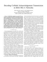
Figure 1: Test images (Image 1 to Image 24, enumerated from left-to-right and top-to-bottom).
High correlation and similarity of detail wavelet coefficients explain the performance gain when denoising in
luminance/color-difference images. The luminance Y is an additive combination of R, G and B color components
and hence preserves the high-frequency image content. On the other hand, the color differences Cb and Cr are
obtained by subtracting the color components: Cb ∝ Y-B and Cr ∝ Y-R. This effectively cancels out high
frequencies, leading to smoother images. These smooth images separate the image signal and noise energy into
low and high frequencies and hence are easier to denoise.
Building on these observations, we make the following contributions:
• We derive an optimal luminance/color-difference space projection that minimizes the noise variance in the
luminance image, leading to better edge preservation. Color-difference images comprise a larger portion
of noise but are smooth and hence can be efficiently denoised without sacrificing the quality.
• We propose a method to estimate the image and noise statistics, necessary to derive the optimal color space
projection, directly from the noisy image data. The estimation approach uses similarity of detail wavelet
coefficients to derive an overconstrained system of linear equations. We then solve this system of equations
for the least squares estimates of the signal variance and the covariance matrix of the noise.
The remainder of the paper is organized as follows. In Section 2 we present a series of experiments that con-
firm strong correlation and similarity of detail wavelet coefficients. Section 3 provides a necessary background
2

Table 1: Pairwise correlation of wavelet coefficients in the three finest scales.
Color R & G R & B G & B
Image Scale LH HL HH LH HL HH LH HL HH
0 0.983 0.993 0.995 0.974 0.991 0.994 0.991 0.996 0.994
1 1 0.978 0.991 0.997 0.969 0.988 0.996 0.992 0.997 0.997
2 0.947 0.968 0.989 0.934 0.954 0.983 0.995 0.995 0.995
0 0.811 0.879 0.969 0.731 0.833 0.963 0.979 0.989 0.980
2 1 0.687 0.834 0.974 0.540 0.755 0.968 0.973 0.985 0.992
2 0.256 0.584 0.857 0.012 0.364 0.822 0.958 0.957 0.985
0 0.942 0.964 0.957 0.880 0.929 0.937 0.887 0.950 0.939
3 1 0.951 0.960 0.974 0.871 0.903 0.952 0.877 0.929 0.962
2 0.917 0.893 0.913 0.737 0.631 0.747 0.767 0.741 0.826
0 0.892 0.967 0.979 0.906 0.970 0.980 0.989 0.993 0.983
4 1 0.878 0.829 0.960 0.895 0.859 0.966 0.991 0.985 0.993
2 0.654 0.637 0.836 0.711 0.698 0.864 0.980 0.977 0.984
0 0.985 0.982 0.989 0.966 0.965 0.984 0.977 0.971 0.979
5 1 0.980 0.975 0.995 0.952 0.950 0.990 0.975 0.967 0.991
2 0.945 0.939 0.970 0.850 0.868 0.929 0.930 0.924 0.963
on wavelet-based denoising. Section 4 proposes an optimal luminance/color-difference projection for image de-
noising. In Sections 5 and 6, we describe the noise estimation procedure and a modified denoising method for
color-difference images. A summary of the proposed denoising method is given in Section 7. Experimental
results are presented in Section 8 to demonstrate the superiority of the proposed method over existing solutions,
both in PSNR and in visual quality. Section 9 concludes the paper and discusses future work.
2 Inter-Color Correlations of High-Frequency Coefficients
Gunturk et al. [22] has shown that high-frequency wavelet coefficients of color components are strongly cor-
related, with correlation coefficients ranging from 0.98 to 1 for most images. This property has been widely
exploited in color filter array (CFA) demosaicking [20]-[26]. In CFA imaging, only one color component is
sampled at each pixel location, and the other color components are interpolated (or demosaicked) from their
neighboring samples. Typical CFA demosaicking methods use color differences to reduce the high-frequency
content of the images, leading to the smoother and hence more suitable signals for interpolation. We replicated
Gunturk’s et al. [22] results for Daubechies-4 wavelet 1 [27] and the three finest scales in Table 1. These results
demonstrate that correlations remain strong even for coarser scales. Here LH, HL and HH are vertical, horizontal
and diagonal detail wavelet subbands, respectively. Overall, the correlation in the HH subband appears to be the
strongest among all the subbands.
In general, perfect correlation between two random variables does not necessarily suggest their equality.
1 Its analysis filters are H0 = (−0.1294, 0.2241, 0.8365, 0.4830), H1(n) = (−1) n H0(4 − n), and synthesis filters are G0(n) =
H0(4 − n), G1 = (−1) n H0(n).
3

However, the observed smoothness in color-difference images means that the high-frequency coefficients of
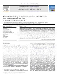
color components are not only correlated but also approximately equal to each other. To demonstrate this we
plotted the 3D scatter diagrams of high-frequency wavelet coefficients in Figure 2. Here, the coordinates of each
point are the magnitudes of the R, G, and B detail wavelet coefficients taken from the same image location of
Image 1 in Figure 1. The points are compactly clustered along the line of vector 1 = (1, 1, 1) T . Similar scatter
diagrams can be obtained for all other test images. These results are similar to Hel-Or’s directional derivatives
scatter plots [24], but are extended to all detail wavelet coefficients and fine scales.
(a) LH, scale 0 (b) HL, scale 0 (c) HH, scale 0
(a) LH, scale 1 (b) HL, scale 1 (c) HH, scale 1
Figure 2: Scatter plots of detail wavelet coefficients. The coordinates of each point are the values of the R, G,
and B components.
The scatter plots also suggest that there exists a more efficient basis capable of compact representation
of the wavelet coefficients. This decorrelation property has been extensively employed in color image com-
pression, by transforming the image from RGB to YCbCr space [28]. Let RGB space correspond to the
standard basis in 3D, then the basis vectors for a typical YCbCr space are v = (0.299, 0.587, 0.114) T ,
d1 = (−0.147, −0.289, 0.436) T and d2 = (0.615, −0.515, −0.100) T [18]. Let x1, x2 and x3 be the values
of the R, G and B detail wavelet coefficients (horizontal, vertical or diagonal) of a particular image location,
4

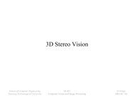
espectively. We call x = (x1, x2, x3) T a signal vector. In Figure 3 we overlay the YCbCr basis vectors on
the scatter plot of all signal vectors. As we can see, vectors d1 and d2 are orthogonal to vector 1. Hence, the
projection of the signal vectors onto d1 and d2 is close to zero. This leads to cancelation of high frequencies and
results in smoother color-difference images that are easier to compress and denoise (see Section 3).
Figure 3: Basis vectors of YCbCr space projection.
Figure 3 also shows that vector v is not aligned with vector 1. The reason is that the luminance Y is chosen to
approximate the grayscale image intensity. This makes YCbCr space backward compatible with the older black-
and-white analog television sets [18]. However, there is a large family of luminance/color-difference spaces, all
having basis vectors d1 and d2 orthogonal to 1, but using different definitions of Y. For example, orthonormal
double-opponent color-difference basis [19] has vector v aligned with 1. However, an efficient basis for a noise-
less image is not necessarily the best for image denoising. This is the topic of Section 4, where we estimate an
optimal space for image denoising from the image noise statistics. To quantify the image denoising performance,
we first introduce several important results from wavelet-based denoising in Section 3.
3 Wavelet-Based Denoising of Grayscale Images
Wavelet denoising is typically based on thresholding and/or shrinkage of wavelet coefficients [2, 7]. The main
idea is to classify high frequency wavelet coefficients into two categories, such as Small and Large, or Noise and
Signal [2], and apply different denoising rules to each category. Let x and ˜x be the wavelet coefficient and its
noisy version, i.e., ˜x = x + n, where n is the noise which is assumed to be zero mean and independent from the
5

signal. let q ∈ {S, L} be the state. Then typical denoising rule for coefficients in state q has the following form:
where β(q) ∈ [0, 1] is the shrinkage coefficient.
ˆx = β(q)˜x (1)
Small coefficients correspond to smooth areas of the image; large coefficients occur near the edges. In a noisy
image the coefficients in smooth areas contain primarily noise; hence such coefficients should be reduced or even
put to zero (β is close to 0). On the other hand, the proportion of the noise in the large coefficients near the edges
is small; hence these coefficients should be preserved (β is close to 1).
Hard assignment rules don’t take into account the uncertainty associated with the state estimation. Better
performance can be achieved by computing for each coefficient the probability that it is affected or unaffected
by noise. The manipulation of the coefficient is then based on this probability. Let p(q|˜x) the conditional state
probabilities. In approach by Pi˘zurica and Philips [11] the shrinkage coefficient was varied according to the ratio
of p(L|˜x) and p(S|˜x). In [4, 5] the wavelet coefficients are modelled as a mixture of two zero-mean Gaussian
distributions with variances σ 2 q + σ 2 n, where σ 2 q and σ 2 n are the signal and noise variances respectively. Then
Minimum Mean Square Error (MMSE) estimate of x is
where
ˆx = p(S|˜x)β(S)˜x + p(L|˜x)β(L)˜x (2)
β(q)˜x =
σ2 q
σ 2 q + σ 2 n
˜x, q ∈ {S, L} (3)
are conditional MMSE estimates. Portilla [6] used a similar framework, but modelled the states via a continuous
scale parameter.
For the hard assignment based denoising, estimation performance depends on the quality of coefficient clas-
sification and the choice of shrinkage coefficient. Smaller noise leads to better classification and hence better
denoising performance. Classification can also be significantly improved by exploiting intra- or inter-scale corre-
lations [9]. Bao and Zhang [8] showed this by applying shrinkage to inter-scale products of wavelet coefficients.
Similarly, for the soft assignment based wavelet denoising, estimation performance depends on the quality
of obtained conditional state probabilities and the choice of shrinkage coefficient. Estimation of conditional state
probabilities can be improved by exploiting inter- and intra-scale correlations, either through constraining the
wavelet coefficient by it local neighborhood of [6], or joint estimation on a tree [4, 5], or using Markov Random
Field modelling [3].
6

Smaller noise also leads to smaller estimation error in conditional MMSE estimates (3). This is the topic of
the following Lemma.
Lemma 1 For a fixed signal variance σ 2 q, the error of conditional MMSE estimate (3) is a non-decreasing func-
tion of error variance σ 2 n.
Proof: From (3) the estimation error variance is
⎡
ε 2 = E (x − ˆx) 2 = E ⎣
σ 2 n
σ 2 q + σ 2 n
x − σ2 q
σ2 q + σ2 n
n
2 ⎤
⎦ = σ2 qσ 2 n
σ 2 q + σ 2 n
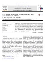
which is a non-decreasing function of σ 2 n for a fixed σ 2 q, as shown in Figure 4.
= σ2 q
σ2 q
σ2 n
Corollary 1 The estimation error variance is always smaller than the signal variance and the noise variance;
i.e.,
∀σ 2 n → ε 2 ≤ σ 2 q, ε 2 ≤ σ 2 n
Corollary 1 explains why it is easier to denoise color differences (Cb and Cr), where suppression of high frequen-
cies leads to small detail wavelet coefficients (or small σ 2 q). Therefore, the estimation error variance is always
small, regardless of how large the noise is, as depicted in Figure 4. This suggests that the denoising performance
can be improved by transforming the image in the color space so that the signal energy is concentrated in one of
the transformed color components. In Section 4 we show that minimizing
The results of Lemma 1 and its corollary are likely to hold even for techniques that don’t use conditional
MMSE estimates. However, the proof will have to be done on a case by case basis and is out of scope of this
paper. Without loss of generality, our experimental results are based on uHMT denoising approach [5].
4 The Optimal Color Space Projection
In Section 2 we showed that detail wavelet coefficients are strongly correlated across image color components,
with the correlation coefficient close to 1. For the sake of simplicity in our following analysis, we assume perfect
correlation, namely
E(xixj) =
+ 1
E(x2 i )E(x2
j ) = s2 i s2 j , ∀i, j (5)
where xi’s are the detail wavelet coefficients in the i-th color component of the noiseless image, and s 2 i ≡ E(x2 i ).
This assumption may not be satisfied exactly in practice and can be relaxed, see Appendix A for the treatment of
the general case of an arbitrary signal covariance matrix.
7
(4)

Estimation error variance
1
0.9
0.8
0.7
0.6
0.5
0.4
0.3
0.2
0.1
0
10 2
10 1
10 0
σ 2
n
10 1
2
σ q = 1
σ 2
q
= 0.1
Figure 4: The estimation error variance as a function of noise variance.
For a typical color image we have s 2 1 s2 2 s2 3 = ¯s2 (see discussion in Section 2). However, the results
derived in this section are applicable to arbitrary signal variances.
Let vector s = (s1, s2, s3) T . We consider a family of luminance/color-difference spaces with basis vectors
(v, d1, d2), where d1 and d2 are orthogonal to s. Our goal is to determine a basis that yields the best denoising
performance. Let xv = v T x be the luminance projection, and xdi = dT i x, i = 1, 2, be the color-difference
projections. Varying the direction of di changes the noise components of xdi
10 2
only; the signal component of
xdi , and hence its variance σ2 q, remains small. This means good denoising performance, as the estimation error
variance ε 2 is always smaller than σ 2 q (see Corollary 1). On the other hand, the luminance xv has a large signal
component. Hence, according to Lemma 1, its denoising performance can be improved by reducing the projected
noise variance.
This observation is illustrated in Table 2, where we apply uHMT denoising to color components in YCbCr
space. Denoising Cb and Cr leads to 6-7 dB better PSNR than denoising Y. Hence, the performance of luminance
denoising, and not that of the color differences, is the key factor in the overall denoising performance.
Our goal is to find a basis (v, d1, d2) with optimal luminance projection for image denoising purpose. Note
that the basis is not orthogonal in general, because d1 and d2 can not be simultaneously orthogonal to v and s.
To simplify the analysis we normalize the coordinates of v = (v1, v2, v3) T so that the variance of the signal
projection onto v is fixed. This is the topic of the following lemma.
Lemma 2 Let x be a random vector that satisfies assumption (5). If we normalize v so that v T s = 1, then the
expected squared norm of the projection of x onto v is always equal to 1 and hence doesn’t depend on v.
8

Table 2: PSNR performance (in dB) of Y, Cb and Cr using the uHMT method in the case of uncorrelated noise.
Color σn = {0.1, 0.1, 0.1} σn = {0.15, 0.1, 0.05}
Image Y Cb Cr Y Cb Cr
1 26.69 37.46 36.68 26.16 38.39 35.69
2 30.96 36.90 35.56 30.59 37.99 34.55
3 30.96 36.43 36.96 30.47 37.81 36.09
4 30.73 37.69 36.14 30.37 38.85 35.16
5 26.80 35.85 36.06 26.18 36.78 35.08
6 27.57 35.99 36.65 26.95 36.15 35.11
7 29.94 36.67 36.78 29.40 37.83 35.80
8 26.48 36.52 35.79 25.42 37.16 34.48
9 30.19 37.04 37.34 29.62 38.06 36.25
10 32.11 37.55 37.51 31.59 38.35 36.41
Average 29.24 36.81 36.55 28.68 37.74 35.46
Proof: Let xv = v T x be the projection of x onto v. Then E(x 2 v) = E(v T xx T v) = v T E(xx T )v. Since the
covariance matrix of the signal is E(xx T ) = ss T , we have E(x 2 v) = v T ss T v = 1.
If the variance of xv is fixed, then choosing the direction of vector v that minimizes the noise projection will
minimize the estimation error of the luminance, as follows from Lemma 1. Yet, this doesn’t guarantee optimality
of v, since the contribution of the luminance component in the inverse formula might depend on v. However, in
Lemma 3 we prove that the constraint v T s = 1 also fixes the contribution of xv in the inverse projection.
Lemma 3 Let x = (x1, x2, x3) T be a random vector that satisfies assumption (5). Let T be an invertible color
projection, such that
⎛
⎜
⎝
xv
xd1
xd2
⎞
⎟
⎠
⎛
⎜
= T ⎜
⎝
x1
x2
x3
⎞
⎛
⎟
⎠ =
⎜
⎝
v T
d T 1
d T 2
⎞ ⎛
⎟ ⎜
⎟ ⎜
⎠ ⎝
where v T s = 1 and d T 1 s = d T 2 s = 0. Then, the corresponding inverse projection is,
where R is a 3 × 2 matrix.
⎛
⎜
⎝
x1
x2
x3
⎞
⎛
⎟
⎠ =
⎜
⎝
s1
s2
s3
⎞
⎟
⎠ xv
⎛
+ R
⎝ xd1
xd2
x1
x2
x3
⎞
⎞
⎟
⎠
(6)
⎠ (7)
Proof: Let T −1 = (r, R), where r is the first column of T −1 . From TT −1 = I it follows that v T r = 1 and
d T 1 r = d T 2 r = 0. Hence, clearly r = s and we obtain (7).
To simplify the inverse projection, we use four basis vectors (one luminance and three color differences)
9

instead of three:
xv = v T x
xdi = xi − sixv = xi − siv T x (8)
One can easily check that so-defined color difference vectors are orthogonal to s. The inverse projection is then
xi = sixv + xdi
Let ˆxi be a denoised version of xi. From (9) it follows that the quality of estimate ˆxi = siˆxv + ˆxdi depends
on v indirectly through the estimation error of ˆxv and ˆxdi . The constraint vT s = 1 fixes the signal variance
of xv according to Lemma 2, and fixes the contribution of xv in the inverse projection according to Lemma 3.
The estimation error of color differences is comparatively small and can be neglected. Hence, choosing v that
minimizes the variance of the luminance noise projection leads to optimal denoising. Lemma 4 relates optimal v
to the signal and noise statistics.
Lemma 4 Let n = (n1, n2, n3) be the noise vector in RGB space and Σn its covariance matrix. Then vector v
with the smallest projected noise variance is
vopt = arg min
vT v
s=1
T Σnv = Σ−1 n s
sT Σ −1
n s
Proof: Let nv = vT n be the projection of n onto v. The variance of nv is E nT
v nv = vT Σnv. According
to Lagrange multiplier method [30], the minimization of v T Σnv under the constraint v T s = 1 is equivalent to
minimization of functional v T Σnv − 2λv T s, where 2λ is the Lagrange parameter. Setting the derivative of the
functional to zero yields
d v T Σnv − 2λv T s
dv
= 2Σnv − 2λs = 0
Solving this equation for v and normalizing the result yields (10).
Figure 5 shows the effect of optimal luminance projection on the denoising performance. Using vopt instead
of v = (0.299, 0.587, 0.114) T from YCbCr leads to better edge preservation and overall image quality.
To obtain vopt we need the noise covariance matrix Σn = E(nn T ), which is typically unknown beforehand.
In Section 5 we discuss how to estimate Σn = E(nn T ) directly from the noisy image data.
10
(9)
(10)

5 Estimation of Noise Covariances
Wavelet coefficients in the HH subband of the finest scale are typically smaller than the coefficients in other
subbands, making it more convenient for noise estimation. For example, in a popular Donoho’s estimator [2], the
standard deviation of the noise is computed as
ˆσn = Median(|˜xi|)
0.6745
where ˜xi are the noisy HH wavelet coefficients. However, in images with fine structures, such as textures, the
HH coefficients are generally larger, leading to potentially inaccurate estimation [8].
Donoho’s estimator can be straightforwardly extended to color images by applying it to each color component
independently. However, this will only produce the estimates of the noise variances and not the noise correlations.
We propose a novel approach capable of estimating the full covariance matrix of the noise, using the similarity
(a) (b) (c)
Figure 5: (a) Noiseless luminance. (b) Denoised luminance using v = (0.299, 0.587, 0.114) T . (c) Denoised
luminance using vopt.
11
(11)

Table 3: Comparison of normalized error of proposed and Donoho’s noise estimator
Noise 2
Uncorrelated Correlated
Uniform Nonuniform Uniform Nonuniform
Covariance matrix Diag. Off-diag. Diag. Off-diag. Diag. Off-diag. Diag. Off-diag.
Donoho’s 0.059 - 0.090 - 0.059 - 0.089 -
Proposed uncorrelated (13) 0.012 - 0.020 - - - - -
Proposed correlated (17) 0.050 0.049 0.089 0.063 0.049 0.033 0.087 0.037
property of detail wavelet coefficients. Unlike Donoho’s approach, our estimates are derived simultaneously for
all color components by solving a system of linear equations. We first discuss the case of uncorrelated noise,
E(ninj) = 0 for i = j, in Section 5.1. A more general case of correlated noise is considered in Section 5.2.
5.1 Estimation of uncorrelated noise variances
Similar to Donoho’s estimator, we use the wavelet coefficients in the HH subband of the finest scale. Table 1
and Figure 2 show that the HH subband coefficients exhibit more similarity than other subbands. We use perfect
correlation assumption (5) and in addition assume that the expected squared norm of the signals is the same for
all color components: E(xixj) = s 2 1 = s2 2 = s2 3 = ¯s2 . Then the covariance matrix of a noisy signal ˜x = x + n
is
⎧
⎨ ¯s
Σ˜x(i, j) = E{˜xi˜xj} =
⎩
2 i = j
where i, j = {1, 2, 3}. Let θ = ¯s 2 , σ 2 n1 , σ2 n2 , σ2 n3
¯s 2 + σ 2 ni i = j
(12)
T be the vector of unknown parameters, and y =
(Σ˜x(1, 1), Σ˜x(2, 2), Σ˜x(3, 3), Σ˜x(1, 2), Σ˜x(1, 3), Σ˜x(2, 1)) T be the data vector. Rewriting (12) in a matrix form
y = B0θ,
we obtain an overconstrained system of 6 equations and 4 unknowns. A least squares estimate (LSE) of θ can be
obtained by using the pseudoinverse of B0 [29]:
ˆθ = B T −1 0 B0 B0y (13)
We applied the Donoho’s estimator and the proposed algorithm to our test images in Figure 1. Table 3 shows
that the normalized average estimation error |ˆσn−σn|
of the proposed algorithm is 4-5 times smaller than the error
σn
of Donoho’s estimator for the case of uncorrelated noise.
2 For the uncorrelated noise, the uniform means equal variance noise added to R, G and B components (σn = {0.1, 0.1, 0.1}),
while the nonuniform means unequal variance noise (σn = {0.15, 0.10, 0.05}). For the correlated noise, the uniform means σn =
{0.10, 0.10, 0.10}, and {0.4, 0.2, 0.3} stands for R&G, R&B, and G&B correlation coefficients respectively. The nonuniform means
12

5.2 Estimation of correlated noise covariances
In general, the noise in different color planes may be correlated:
Σn(i, j) = σ 2 ni,j = E {ninj} = 0, i = j
For example, a high temperature can cause excessive thermal noise on a color sensor. The noise is temperature
dependent and hence is likely to be similar in the local neighborhood of the color sensors [32]. In this case,
assuming uncorrelated noise and using estimate (13) can lead to poor estimates of the luminance basis vector
vopt and hence poor denoising performance, as shown in Table 6.
For correlated noise we can rewrite (12) as
⎧
⎨
Σ˜x(i, j) =
⎩
¯s 2 + σ 2 ni,j i = j
¯s 2 + σ 2 ni
where i, j = {1, 2, 3}. Let θ be the vector of seven unknown parameters (signal variance, three noise variances,
and three noise covariances). Rewriting (14) in a matrix form yields
y = B1θ
This is an underconstrained system with 6 equations and 7 unknowns. To provide additional constraints we use
Donoho’s estimator (11) for σ 2 ni ’s, thus adding three more equations to (14). Let y d be the vector of Donoho’s
estimated noise variances:
i = j
(14)
y d = Aθ (15)
Since Donoho’s estimator is not as accurate as (14), we take (14) as a constraint and obtain a constrained LSE
estimate of (15):
ˆθ = arg min
y=B1θ (y d − Aθ) T (y d − Aθ) (16)
According to Theorem 19.2.1 in [31], ˆ θ is the first part of the solution to the following system of linear equations:
⎛
⎝ A BT 1
B1 0
⎞ ⎛
⎠ ⎝ θ
⎞ ⎛
⎠ =
r
⎝ AT y d
y
σn = {0.05, 0.15, 0.10}, with correlations {0.3, 0.3, 0.3}. The same types of noise are used further in the paper.
13
⎞
⎠

Hence,
⎛
⎝ ˆ θ
r
⎞
⎠ =
⎛
⎝ A BT 1
B1 0
⎞
⎠
−1 ⎛
⎝ AT y d
y
⎞
⎠ (17)
Table 3 shows the estimation performance of the proposed estimator (17) on the diagonal and off-diagonal
entries of the noise covariance matrix. Performance on the diagonal entries is similar to that of the Donoho’s
estimator. The non-diagonal entries are estimated equally well. Hence the estimator (17) can be used in the case
when it is unknown a priori whether the noise is correlated or not.
Even though the assumptions of perfect signal correlation and uniform variances may not be satisfied in real
life, experimental results suggest that estimator (17) is sufficiently precise for the optimal luminance projection-
based wavelet denoising, see Table 6. The PSNR performance is only 0.3-dB worse compared to using exact
noise covariance matrix.
6 Denoising of Color-Difference Images
Statistical description of the optimal luminance projection resembles that of grayscale images. Hence the standard
grayscale image denoising approaches can be straightforwardly applied to luminance denoising. On the other
hand, the color-difference components are much smoother, and might require some modifications to the existing
grayscale approaches. The modifications are likely to be algorithm dependent and should be decided on a case
by case basis. We consider this problem on the example of uHMT denoising approach.
Compared to grayscale images, the edges of color difference images are smaller in amplitude, leading to
smaller detail wavelet coefficients in the fine scales. For a sufficiently noisy image, the the signal variance in these
scales is much smaller than the noise variance, σ 2 S < σ2 L ≪ σ2 n. This leads to the following two observations:
1. The variances of noisy coefficients in two states are similar to each other, i.e. σ 2 S + σ2 n ≈ σ 2 L + σ2 n, making
it difficult to distinguish these coefficients
2. The shrinkage parameters corresponding to conditional MMSE estimates are close to zero:
σ 2 S
σ 2 S + σ2 n
≈ 0,
σ 2 L
σ 2 L + σ2 n
≈ 0 (18)
The first observations is likely to lead to misclassification of fine scale coefficients. Since the conditional dis-
tributions of large and small coefficients are close to each other, the prior state probabilities p(S), p(L) will be
the deciding factor in computing conditional state probabilities p(q|˜x). Since for a typical image p(S) ≫ p(L),
14

hence p(S|˜x) ≫ p(L|˜x) for a large range of ˜x. This observation is supported by experiment in Figure 6(b):
classifying coefficients according to conditional state probabilities puts an overwhelming majority of fine scale
coefficients into the Small state.
On the other hand, the detail wavelet coefficients in the coarser scales are still large and should allow for a
good separation of large and small coefficients. However, contrary to our expectations, an overwhelming majority
of the coarse-scale coefficients are also classified as small, as shown in Figure 6(b). This can be explained by a
tie between the neighboring scales, which is introduced to exploit the inter-scale correlations [4, 8]. The original
idea of scale connections was primarily for coarser scale coefficients to help classification of the finer scale ones.
In color difference images we obtain an opposite effect - wrongly classified fine scale coefficients adversely affect
the classification in coarser scales.
We propose to resolve this problem by separating the fine and coarse scales using the following simple test:
⎧
⎨
⎩
F ine ˆσ 2 di ≤ tˆσ2 n
Coarse ˆσ 2 di > tˆσ2 n
where ˆσ 2 di and ˆσ2 n are signal and noise variances, estimated from noisy image data, and t is the tolerance parameter
chosen empirically. If the noise dominates the signal, we set the scale as Fine, otherwise we set it as Coarse.
For simplicity we treat all fine scale coefficients as small, since the conditional denoising rules are similar to
each other according to (18). The denoising in coarse scales is done in the same way as before. Scale separation
yields much better classification and denoising performance, as shown in Figure 6(c)(d) and Table 4. In particular,
the proposed modification yields an average PSNR gain of 3 dB in color difference images.
(a) (b) (c) (d)
Figure 6: (a) Color-difference image. The sates of wavelet coefficients (b) after uHMT denoising, (c) after uHMT
denoising with Fine/Coarse-Scale separation, and (d) in coarse scale after uHMT denoising with Fine/Coarse-
Scale separation; gray and white pixels correspond to small and large coefficient states, respectively.
15
(19)

Table 4: PSNR performance (in dB) of uHMT on color-difference images with and without Fine/Coarse-scale
separation
Color σn = {0.1, 0.1, 0.1} σn = {0.15, 0.1, 0.05}
Image Without F/C F/C Without F/C F/C
1 Cb 37.46 41.74 38.39 42.53
Cr 36.68 39.56 35.69 38.66
2 Cb 36.90 39.35 37.99 40.71
Cr 35.56 36.59 34.55 34.75
3 Cb 36.43 38.66 37.81 40.06
Cr 36.96 41.05 36.09 39.78
4 Cb 37.69 43.34 38.85 44.38
Cr 36.14 37.84 35.16 36.88
5 Cb 35.85 36.86 36.78 37.60
Cr 36.06 37.43 35.08 36.48
Average Cb 36.87 39.99 37.96 41.06
Cr 36.28 38.49 35.32 37.31
7 Summary of the Proposed Denoising Method
The proposed optimal color projection (OCP) based denoising method consists of the following four key steps:
1. For a given RGB image, use (17) to estimate the covariance matrix of the noise Σn. If the noise is known
to be uncorrelated, then estimator (13) can be used to achieve slightly better performance.
2. Use ˆ Σn and (10) to derive the optimal color projection. Applying it to the original RGB image yields the
optimal projection of luminance ˜xopt and color differences ˜xdi , as defined in (8).
3. Apply the uHMT (or any other grayscale denoising approach) to new color components. If necessary,
modify the algorithm to suit the properties of color differences, as we did with uHMT by Fine/Coarse-
scale separation.
4. Reconstruct the RGB color components using the inverse color projection (9).
Note that the proposed scheme is not constrained by the uHMT denoising approach. Applying optimal projection
to other popular wavelet-based denoising approaches leads to similar performance improvement, as shown in
Section 8.2.
The complexity of the proposed denoising algorithm primarily depends on the adopted denoising method, and
hence is increased by a factor of three-four (depending on the number of color difference components) compared
to grayscale image denoising. The complexities of noise estimation and color projection steps are relatively
small.
16

Table 5: Comparison of CPSNR performance (in dB) of uHMT in RGB, YCbCr, and proposed OCP color spaces
Uncorrelated noise Correlated noise
Uniform Nonuniform Uniform Nonuniform
RGB 27.11 27.19 27.17 27.25
YCbCr 28.22 27.78 27.63 26.91
OCP 28.79 29.51 27.94 29.02
Table 6: Comparison of CPSNR performance (in dB) of Donoho’s and proposed noise estimators
Uncorrelated noise Correlated noise
Uniform Nonuniform Uniform Nonuniform
Donoho 28.92 29.67 27.53 28.92
Proposed 29.17 29.81 28.21 29.31
exact 29.17 29.90 28.28 29.51
8 Experimental Results and Discussion
In our experiments we use 24 test color images shown in Figure 1. As a performance measure we adopt the color
peak signal-to-noise ratio (CPSNR), defined as the average Mean Square Error (MSE) of the denoised color
components, CPSNR = −10 log( 1
3
c∈{R,G,B} MSEc), for normalized to [0, 1] RGB values.
8.1 Performance contributions of proposed algorithm components
Our proposed algorithm, when coupled with uHMT, consists of three main components (Section 7): optimal color
projection (OCP), noise estimator, and denoising of color difference images with separating Fine/Coarse scales
(F/C). In this section we show the effect of each individual component on the resultant denoising performance.
To demonstrate the effect of color projection we compare the average CPSNR performance of applying
uHMT in RGB, YCbCr and the proposed OCP color spaces in Table 5. Denoising in OCP substantially outper-
forms denoising in RGB, by an average of 0.8-2.3dB depending on the relative noise distribution. The difference
between denoising in OCP and YCbCr is more subtle. Average OCP gain over YCbCr is only 0.3-0.6dB for
uniform noise. This can be explained by the similarity of the optimum luminance projection vector and vector
Y = (0.299, 0.587, 0.114) from YCbCr under the uniform noise. However, the performance gain grows up to
1.6-2.1dB for the case of non-uniform noise.
The proposed noise estimation technique also has substantial effect on the overall denoising performance,
especially for the correlated noise. According to results in Table 6, our method outperforms the Donoho’s by
0.15-0.3dB for the uncorrelated noise and by 0.4-0.7dB for the correlated noise. Moreover, this performance is
only about 0.15dB worse compared with the case when exact noise covariance matrix is known.
The proposed separation of Fine/Coarse scale (F/C) in uHMT substantially improves the denoising perfor-
17

Table 7: Comparison of CPSNR performance (in dB) with or without separating Fine/Coase scales (F/C) in
denoising color different images.
Uncorrelated noise Correlated noise
Uniform Nonuniform Uniform Nonuniform
without F/C 28.79 29.51 27.94 29.02
with F/C 29.17 29.81 28.21 29.31
Table 8: CPSNR performance (in dB) by applying OCP into different approaches for grayscale images.
Uncorrelated noise Correlated noise
Uniform Nonuniform Uniform Nonuniform
RGB 27.03 26.95 27.03 26.99
Hard-Thr YCbCr 28.30 27.84 27.71 26.88
OCP 28.73 29.35 27.93 29.19
RGB 27.59 27.48 27.59 27.51
Soft-Thr YCbCr 28.77 28.31 28.19 27.38
OCP 29.21 29.75 28.45 29.54
RGB 27.80 27.72 27.67 27.60
GSM YCbCr 28.90 28.46 28.31 27.52
OCP 29.72 30.44 28.62 29.74
mance of color difference images. The color difference images contribute less to the overall denoising perfor-
mance compared to the luminance. Overall improvement is 0.3-0.4 on average, as shown in Table 7).
In summary, color projection is the main factor in the overall denoising performance improvement, followed
by the noise estimation and the adaption of denoising to color differences. The improvements are already notice-
able for images with uniform uncorrelated noise and become quite substantial in image with correlated and/or
nonuniform noise.
8.2 OCP with other grayscale wavelet-based denoising approaches
The proposed OCP can be combined with any grayscale wavelet-based denoising approach. In Table 8 we show
the results of combining OCP with several existing approaches. In this table, Hard-Thr and Soft-Thr are hard
and soft thresholding of wavelet coefficients proposed in [7]. GSM stands for denoising based on Gaussian Scale
Mixtures model, proposed by Portilla et al [6]. We used redundant wavelet transform in Hard-Thr and Soft-Thr,
and orthogonal wavelet transform in GSM. The observed performance gains are similar to the ones we observed
in uHMT (Table 5).
18

8.3 Comparison to existing state-of-the-art methods
We also compared the proposed OCP denoising with three state-of-the-art methods, wiener filtering wiener2 3 ,
and two recently proposed wavelet-based denoising methods, LSAI 4 [11], MML [13] 5 . For fairness, we adopt
an orthogonal wavelet transform for all wavelet-based tested approaches. As shown in Table 9, the proposed
approach outperforms all others on every test image.
In particular, for uniform noise, the average CPSNR gains of RGB is 3dB, 1.7dB, and 1dB over wiener2,
LSAI, and MML respectively, as shown in Table 10. Even larger gains are achieved for nonuniform noise, where
average PSNR gain for the noisiest component becomes 5dB, 2.7dB, and 1.9dB.
Table 9: CPSNR performance (in dB) of wiener2, LSAI, MML, and OCP methods.
Uncorrelated noise Correlated noise
Color Uniform Nonuniform Nonuniform
Image wiener2 LSAI MML Ours wiener2 LSAI MML Ours wiener2 LSAI MML Ours
1 24.71 25.25 26.67 27.42 24.36 25.26 27.42 28.73 24.40 25.11 26.93 27.48
2 27.03 29.17 29.20 30.22 26.30 29.07 29.20 30.48 26.73 29.16 29.50 30.14
3 26.87 29.34 29.43 30.54 26.35 29.19 29.66 30.76 26.38 29.14 29.60 30.97
4 26.90 29.10 29.34 30.41 26.33 29.08 29.56 30.85 26.46 29.04 29.41 30.39
5 25.30 24.98 26.47 27.11 24.94 24.94 27.02 28.11 24.93 24.86 26.62 27.34
6 25.13 25.89 27.21 28.01 24.71 25.74 27.37 28.66 24.74 25.76 27.41 28.59
7 26.84 27.93 28.51 29.74 26.30 27.96 28.95 30.46 26.29 27.75 28.73 30.01
8 24.12 25.00 26.40 27.04 23.78 24.88 26.93 28.13 23.83 24.77 26.71 27.39
9 26.71 28.23 28.98 30.24 26.18 28.10 29.32 30.72 26.15 27.97 29.22 30.77
10 27.15 30.55 30.28 32.08 26.53 30.24 30.30 32.63 26.56 30.23 30.46 32.56
11 26.12 26.99 27.95 29.02 25.69 26.90 28.41 29.79 25.60 26.85 28.11 29.27
12 27.00 29.67 29.58 31.04 26.40 29.61 29.70 31.59 26.44 29.18 29.32 30.89
13 24.31 24.10 26.08 26.52 23.94 24.22 26.80 27.80 23.96 24.10 26.06 26.28
14 26.32 26.72 27.56 28.23 25.83 26.59 27.78 28.50 25.82 26.66 27.75 28.42
15 26.94 28.78 28.86 29.96 26.31 28.62 28.80 30.16 26.36 28.37 28.34 29.48
16 26.66 29.05 29.53 30.83 26.17 28.96 29.73 31.70 26.15 28.90 29.73 31.52
17 26.93 28.37 28.84 30.23 26.37 28.32 29.11 31.00 26.25 27.96 28.38 30.24
18 26.37 26.38 27.49 28.19 25.85 26.33 27.76 28.93 25.91 26.33 27.73 28.53
19 25.43 26.53 27.73 28.39 24.97 26.31 27.99 29.16 25.05 26.35 28.15 29.02
20 26.47 27.21 27.39 28.45 25.58 26.63 26.81 28.03 25.77 26.80 26.16 27.37
21 25.85 26.55 27.86 28.76 25.39 26.50 28.32 29.66 25.43 26.43 28.25 28.70
22 26.47 27.49 28.09 28.90 25.86 27.40 28.25 29.54 26.01 27.42 28.35 29.05
23 27.28 30.25 30.13 31.40 26.64 29.93 30.06 31.46 26.70 29.75 30.23 31.32
24 25.68 25.73 26.82 27.52 25.12 25.77 27.19 28.65 25.18 25.50 26.97 27.57
Average 26.19 27.47 28.18 29.17 25.66 27.36 28.44 29.81 25.71 27.27 28.25 29.31
We can provide a simple intuition explaining the outstanding performance of the proposed OCP denoising,
especially on images with non-uniform noise. Existing denoising techniques, such as wiener2, LSAI or grayscale
3
The spatial filtering, the function “wiener2” in MATLAB is used.
4
We used the software provided by the authors with a minor modification to allow for different noise variances in the R,G and B
components.
5
The paper mentions two alternative parameter estimation, using MAP or ML framework. We adopted the latter one since it yields
better CPSNR.
19

Table 10: Average PSNR performance (in dB) of RGB from wiener2, LSAI, MML, and OCP methods.
Uncorrelated noise Correlated noise
Uniform Nonuniform Nonuniform
wiener2 LSAI MML Ours wiener2 LSAI MML Ours wiener2 LSAI MML Ours
R 26.11 27.59 28.20 29.23 23.23 25.88 26.72 28.63 30.22 29.87 30.93 30.94
G 26.15 27.60 28.34 29.43 26.15 27.61 29.00 30.45 23.30 25.84 26.84 28.68
B 26.22 27.86 28.49 29.59 30.30 30.41 31.58 31.82 26.23 27.69 28.70 29.65
approaches in YCbCr assign approximately equal weight to each color component. In the proposed OCP denois-
ing, less noisy channels have larger weight in the final reconstruction. This results in better denoising, since
smaller noise leads to smaller estimation error according to Lemma 1.
Another advantage of the proposed OCP denoising method is better edge preservation. To show this we
partition the image into two regions corresponding to edges and smooth areas, and compare their denoising per-
formance. We use Canny edge detection [33] followed by thresholding to obtain the classification. Table 11
shows the CPSNR of the two regions for wiener2, LSAI, MML, and OCP methods. LSAI uses intra-scale corre-
lations and hence outperforms wiener2 in smooth regions. However, both algorithms achieve similar performance
in the edge regions. The proposed OCP denoising is superior to both LSAI and wiener2, outperforming LSAI by
2-3 dB in edge regions and by 1-1.5 dB in smooth regions. MML denoising fairs well in the edge region, but still
about 0.35-0.9dB worse compared to OCP. However, its performance in the smooth regions is quite poor, even
compared to the LSAI approach.
The visual quality improvements are even more striking than the PSNR gains. We applied the wiener2, LSAI,
MML, uHMT on YCbCr and uHMT on OCP to several test images. The results are shown in Figures 7, 8, and
9. The proposed OCP denoising leads to much fewer color artifacts and better edge preservation compared with
the other methods.
Figure 7 shows an image of a fence. The OCP denoising preserves edges better than the other methods, while
almost completely removing the color artifacts. MML also produces sharp edges, but fails in the smooth regions.
Similar observations can be made for the image of a bird in Figure 8. The LSAI oversmoothes the cheek area
but reveals some color artifacts in the area above the eye. The OCP preserves the cheek texture and successfully
removes the artifacts. An example of the OCP’s superior edge preservation is shown in Figure 9. In the original
image there are several parallel background thin lines that go across the wheel. The OCP denoising is the only
method that preserves these lines without introducing color artifacts in the smooth areas.
20

(a) Origin image (b) Noisy image
(c) wiener2 (d) LSAI
(e) MML (f) Ours
Figure 7: Comparison of different denoising approaches on the fence image corrupted by uncorrelated nonuniform
noise.
21

(a) Origin image (b) Noisy image
(c) wiener2 (d) LSAI
(e) MML (f) Ours
Figure 8: Comparison of different denoising approaches on the parrot image corrupted by uncorrelated nonuniform
noise.
22

Table 11: CPSNR performance (in dB) in the edge (E) and smooth (S) image regions.
Uncorrelated noise Correlated noise
Color Uniform Nonuniform Nonuniform
Image wiener2 LSAI MML Ours wiener2 LSAI MML Ours wiener2 LSAI MML Ours
1 E 23.28 23.67 25.81 26.15 23.06 23.60 26.71 27.78 23.06 23.50 25.95 26.19
S 26.54 27.37 27.59 28.92 25.94 27.54 28.15 29.81 26.06 27.27 28.02 28.99
2 E 25.93 26.61 27.69 28.28 25.46 26.55 27.88 28.87 25.65 26.73 27.89 28.49
S 27.87 32.10 30.48 32.07 26.90 31.91 30.27 31.94 27.54 31.82 30.89 31.64
3 E 25.42 25.86 27.24 27.65 25.10 25.78 27.68 27.89 25.13 25.86 27.47 28.26
S 27.71 32.76 30.92 32.86 27.04 32.46 30.95 32.91 27.08 32.15 31.02 33.01
4 E 25.97 26.63 27.88 27.29 25.57 26.66 28.32 29.09 25.72 26.77 28.07 28.65
S 27.60 31.93 30.59 31.23 26.88 31.80 30.57 32.50 27.00 31.48 30.52 32.04
5 E 23.79 23.28 25.53 25.78 23.55 23.19 26.25 26.96 23.53 23.20 25.52 25.95
S 27.31 27.38 27.51 28.76 26.70 27.45 27.84 29.48 26.72 27.18 27.91 29.07
6 E 23.48 23.99 26.05 26.47 23.21 24.02 26.66 27.72 23.25 23.92 26.41 27.30
S 27.18 28.45 28.46 29.94 26.47 27.91 28.05 29.61 26.49 28.19 28.44 30.01
7 E 25.33 25.16 26.84 27.43 25.00 25.27 27.53 28.44 25.02 25.12 27.01 27.80
S 27.92 30.72 29.76 31.66 27.18 30.59 29.94 32.10 27.15 30.28 30.02 31.86
8 E 22.38 23.30 25.31 25.45 22.13 23.21 26.15 26.97 22.17 23.00 25.55 25.65
S 25.81 26.64 27.31 28.49 25.32 26.47 27.52 29.08 25.40 26.50 27.67 28.22
9 E 25.13 25.33 27.22 27.84 24.80 25.30 27.85 28.72 24.77 25.20 27.46 28.54
S 27.86 31.27 30.31 32.41 27.13 30.93 30.36 32.31 27.11 30.75 30.55 32.74
10 E 25.89 26.57 28.13 28.87 25.49 26.38 28.52 29.73 25.53 26.49 28.36 29.25
S 27.68 33.60 31.34 34.05 26.94 33.10 31.11 34.37 26.97 32.90 31.48 34.47
11 E 24.53 24.55 26.46 26.21 24.26 24.43 27.13 28.00 24.23 24.54 26.75 27.49
S 27.61 29.95 29.30 29.27 26.98 29.93 29.52 31.60 26.81 29.52 29.30 31.02
12 E 26.06 27.54 28.40 29.35 25.65 27.72 28.86 30.33 25.64 27.18 28.30 29.39
S 27.70 31.85 30.51 32.64 26.95 31.41 30.32 32.68 27.02 31.15 30.09 32.16
Average E 24.76 25.21 26.88 27.23 24.44 25.18 27.46 28.37 24.47 25.13 27.06 27.75
S 27.40 30.34 29.51 31.03 26.70 30.13 29.55 31.53 26.78 29.93 29.66 31.27
9 Conclusions and Future Work
Exploiting inter-color correlations can improve the performance of color image denoising. In this paper we
developed a novel denoising approach that is based on similarity of detail wavelet coefficients across the color
components. The denoising is done by projecting the image onto an optimal luminance/color-difference space
adapted to image noise. The projection minimizes the noise in the luminance component, thus preserving the
high-frequency contents of the image. On the other hand, the color-difference components are smooth and can
be easily denoised regardless of the amount of noise present.
Another contribution of this paper is a novel approach to estimation of the inter-color covariance matrix of
the noise that is used to determine the optimal color projection. The proposed estimator is shown to be more
accurate than the popular Donoho’s estimator in the case of uncorrelated noise. It also demonstrates remarkable
performance for correlated noise across the color components.
Experimental results suggest that the proposed optimal color projection (OCP) denoising method outperforms
23

the existing solutions not only in PSNR but also in visual quality. In particular, the OCP denoising demonstrates
superior edge preservation properties while removing almost all color artifacts.
In the current work we have exploited inter-color correlations, but assumed the noise to be uncorrelated
between the pixels of the same color component. In the future we plan to extend the proposed algorithm to take
into account the noise correlations between neighboring pixels.
A Optimal color projection for arbitrary signal covariance matrix
In Section 4 we assumed perfect correlation between detail wavelet coefficients of RGB color components. In
this section we explain how to relax this assumption to an arbitrary covariance matrix Σx. The direction that
preserves energy of the signal is given by the eigenvector of Σx corresponding to largest eigenvalue. Let u0 be
such an eigenvector. It’s easy to check that u0 is a generalization of the signal vector s, since u0 = s when
Σx = ss T . New color difference projection vectors, d1 and d2, are defined as orthogonal to u0.
By normalizing the luminance projection vector v by v T u0 = 1 we satisfy the conditions of Lemma 3. The
so defined basis (v, d1, d2) fixes the contribution of the luminance xv = v T x in the inverse projection. The
estimation error of color differences is comparatively small and can be neglected. Hence, choosing the optimal
v for the luminance noise projection leads to optimal denoising.
However, unlike in the perfect correlation case, the constraint v T u0 = 1 does not fix the variance of xv.
Hence, instead of minimizing the noise projection, we seek a projection that maximizes the signal-to-noise ratio
(SNR). The variance of the signal and the noise projections onto a vector v are E[(v T x) 2 ] = v T Σxv and
E[(v T n) 2 ] = v T Σnv respectively. The following Lemma shows how to obtain v that maximizes ratio vT Σxv
v T Σnv .
Lemma 5 The optimal vector v that yields the largest SNR projection is the eigenvector of the matrix Σ −1
n Σx
corresponding to the largest eigenvalue.
Proof: Setting the derivative of vT Σxv
vT Σnv
to zero yields
d
vT Σxv
vT
Σnv
dv
= 0 ⇛ Σ −1
n Σxv = vT Σxv
v T Σnv v
Hence the necessary condition for v is to be an eigenvector of Σ −1
n Σx. Let Σ −1
n Σxv = λv. Then
vT Σxv
vT Σnv = vT Σnλv
vT Σnv
24
= λ

Table 12: CPSNR performance (in dB) using the perfect correlation assumption vs arbitrary signal covariance
matrix
Uncorrelated noise Correlated noise
Uniform Nonuniform Uniform Nonuniform
Arbitrary 29.23 29.92 28.29 29.49
Assumption 29.19 29.89 28.28 29.51
Setting v to an eigenvector corresponding to the largest eigenvalue maximizes vT Σxv
vT Σnv
and hence the SNR.
One can check that vector v obtained using Lemma 5 coincides with the one obtained by Lemma 4 when
Σx = ss T .
Signal covariance matrix varies across subband and scales. Hence one can potentially use a different color
projection for each subband and scale of the wavelet tree. However, the main problem here is to estimate the
noise and signal covariance matrices simultaneously. If the noise covariance matrix is known beforehand, the
signal covariance matrix can be estimated using
ˆΣx = E(˜x˜x T ) − Σn
Applying color projection to each scale increases the computational complexity but leads to only modest
improvements in the denoising performance, as shown in Table 12. The difference between CPNSR doesn’t
exceed 0.04dB.
25
(20)

(a) Origin image (b) Noisy image
(c) wiener2 (d) LSAI
(e) MML (f) Ours
Figure 9: Comparison of different denoising approaches on the digital camera test image corrupted by correlated
nonuniform noise.
26

References
[1] A. K. Jain, “Fundamentals of digital image processing”, Prentice Hall, 1989.
[2] D. L. Donoho and I. M. Johnstone, “Adapting to unknown smoothness via wavelet shrinkage,” J. Amer.Statist.Assoc.,, vol. 90, pp.
1200-1224, 1995.
[3] M. Malfait and D. Roose, “Wavelet-based image denoising using a Markov Random Field a prior model,” IEEE Trans. on Image
Processing, vol. 6, no. 4, pp. 549-565, Apr 1997.
[4] M. S. Crouse, R. D. Nowak and R. G. Baraniuk, “Wavelet-based statistical signal processing using Hidden malkov Models,” IEEE
Trans. on Signal Processing, vol. 46, no. 4, pp. 886-902, Apr 1998.
[5] J. Romberg, H. Choi and R. G. Baraniuk, “Bayesian tree-structured image modeling using wavelet-domain Hidden Markov Models,”
IEEE Trans. on Image Processing, vol. 10, no. 7, pp. 1056-1068, July 2001.
[6] J. Portilla, V. Strela, M. J. Wainwright, and E. P. Simoncelli, “Image Denoising Using Scale Mixtures of Gaussians in the Wavelet
Domain,” IEEE Trans. on Image Processing, vol. 12, no. 11, Nov 2003.
[7] M.Lang, H.Guo, J. E.Odegard, C. S.Burrus, and R. O.Wells, “Noise reduction using an undecimated discrete wavelet transform” ,
IEEE Signal Processing Letter, vol. 3, pp. 10-12, Jan. 1996.
[8] P. Bao and L. Zhang, “Noise reduction for magnetic resonance images via adaptive multiscale products thresholding,” IEEE Trans.
on Medical Imaging, vol. 22, no. 9, pp. 1089-1099, Sep 2003.
[9] J. Liu and P. Moulin, “Information-theoretic analysis of interscale and intrascale dependencies between image wavelet coefficients
” IEEE Trans. on Image Processing, vol. 10, no. 11, Nov 2001.
[10] P. Scheunders, “Wavelet thresholding of multivalued images,” IEEE Trans. on Image Processing, vol. 13, no. 4, pp. 475-483, Apr
2004.
[11] A. Pi˘zurica and W. Philips, “Estimating probability of presence of a signal of interest in multiresolution single- and multiband
image denoising,” to appear in IEEE Trans. on Image Processing.
[12] A. Pi˘zurica, “Image denoising using wavelets and spatial context modeling,” Ph.D. thesis, Ghent University, June 2002.
[13] P. Scheunders, J, Driesen,“Least-squares interband denoising of color and multispectral images,” IEEE Int. Conf. Image Processing,
Singapore, Oct 2004.
[14] O. Ben-Shahar and S. W. Zucher “Hue fields and color curvatures: a perceptual organization approach to color image denoising,”
IEEE conference on CVPR, June 2003.
[15] T. F. Chan, S. H. Kang, and J. Shen “Total Variation Denoising and Enhancement of Color Images Based on the CB and HSV Color
Models,” Journal of Visual Communication and Image Representation, vol. 12, pp. 422-435, June 2001.
[16] B. Tang and V. Caselles, “Color Image Enhancement via Chromaticity Diffusion,” IEEE Trans. on Image Processing, vol. 10, no.
5, pp. 701-707, May 2001.
[17] S. Kim and S. H. Kang, “Implicit Procedures for PDE-based Color Image Denoising via Brightness-Chromaticity Decomposition,”
Technical Report, Department of Mathematics, University of Kentucky, Lexington, KY, July 2002.
[18] C. A. Poynton, “A technical introduction to digital video,” John Wiley & Sons, Inc., 1996.
[19] B. Wandell, “Foundations of vision,” Sinaur Associates, 1995.
27

[20] J. F. Hamilton and J. E. Adams, “Adaptive color plane interpolation in single sensor color electronic camera,” U.S. Patent, no.
5,629,734, 1997.
[21] S. C. Pei and I. K. Tam, “Effective color interpolation in CCD color filter array using signal correlation,” IEEE Int. Conf. Image
Processing, vol. 3, 2000.
[22] B. K. Gunturk, Y. Altunbasak and R. M. Mersereau, “Color plane interpolation using alternating projections,” IEEE Trans. on Image
Processing, vol. 11, no. 9, pp. 997-1013, Sep 2002.
[23] L. Chang and Y.-P. Tan, “Effective use of Spatial and Spectral Correlations for Color Filter Array Demosaicking,” IEEE Trans. on
Consumer Electronics, vol. 50, no. 1, pp. 355-365, Feb 2004.
[24] Y. Hel-Or, “The Canonical Correlations of Color Images and their use for Demosaicing,” Technical Report, HP Labs, HPL-2003-
164R1, Feb 2004.
[25] X. Wu and N. Zhang, “Primary-consistent soft-decision color demosaicking for digital cameras,” IEEE Trans. on Image Processing,
vol. 13, no. 9, pp. 1263-1274, Sep 2004.
[26] D. D. Muresan and T. P. Parks, “Demosaicking using optimal recovery,” IEEE Trans. on Image Processing, vol. 14, no. 2, pp.
267-278, Feb 2005.
[27] I. Daubechies, ”Orthonormal bases of compactly supported wavelets,” Communications on Pure and Applied Mathematics, vol. 16,
pp. 909-996, Jan 1988.
[28] V. Bhaskaran and K. Konstantinides, “Image and video compression standards”, Kluwer Academic Publishers, 1995.
[29] B. Widrow, and S. Stearns, “Adaptive signal processing,” New Jersey, Prentice Hall, 1990.
[30] D. P. Bertsekas, “Constrained optimization and Lagrange multiplier methods,” New York, Academic Press, 1982.
[31] D. A. Harville, “Matrix algebra from a statistician’s perspective,” New York, Springer, 1997.
[32] G. C. Holst, “CCD Arrays cameras and displays,” JCD Publishing and SPIE Optical Engineering Press, 1998.
[33] J. F. Canny, “A computational approach to edge detection”, IEEE Trans. on Pattern Analysis and Machine Intelligence, vol. 8, no.
6, pp. 679-698, Nov 1986.
28