Download - Arab Journal of Nuclear Sciences and Applications
Download - Arab Journal of Nuclear Sciences and Applications
Download - Arab Journal of Nuclear Sciences and Applications

Create successful ePaper yourself
Turn your PDF publications into a flip-book with our unique Google optimized e-Paper software.
<strong>Arab</strong> <strong>Journal</strong> Of <strong>Nuclear</strong> Science And <strong>Applications</strong>, 46(2), (276-286) 2013<br />
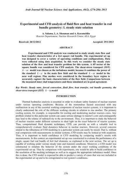
Experimental <strong>and</strong> CFD analysis <strong>of</strong> fluid flow <strong>and</strong> heat transfer in rod<br />
bundle geometry: I. steady state solution<br />
A. Salama, L.A. Shouman <strong>and</strong> A. Karameldin<br />
Reactor Departement, <strong>Nuclear</strong> Research Center, AEA, Egypt<br />
Received: 20/12/2012 Accepted: 29/1/2013<br />
ABSTRACT<br />
Experimental <strong>and</strong> CFD analysis was conducted to study steady state flow <strong>and</strong><br />
heat transfer characteristics <strong>of</strong> a 4x4 square rod bundle. The experimental set up<br />
was designed to cover a variety <strong>of</strong> operating conditions <strong>and</strong> configurations. Data<br />
were collected using data acquisition. In this work we consider the steady state<br />
solution <strong>of</strong> the flow <strong>and</strong> heat transfer problem for this system. A 45o-sector <strong>of</strong> the<br />
square bundle was considered for CFD analysis. The shear-stress transport (SST)<br />
k <br />
model was chosen as the turbulence model, because it combines the power <strong>of</strong><br />
the st<strong>and</strong>ard <br />
k in the main flow field <strong>and</strong> the st<strong>and</strong>ard <br />
276<br />
k model in the<br />
near wall regions. Fine meshes were considered in the boundary layer region to<br />
accurately capture the basic characteristics <strong>of</strong> the flow field. Comparisons between<br />
the measured inner clad temperatures <strong>and</strong> those simulated are in good agreement.<br />
Key Words: Steady state, forced convection, fluid flow, heat transfer, rod bundle geometry, the<br />
shear-stress transport (SST) <br />
k model<br />
INTRODUCTION<br />
Thermal hydraulics analysis is essential in order to evaluate safety features <strong>of</strong> nuclear reactors<br />
under various operating conditions. Because <strong>of</strong> the tremendous hazard associated with any<br />
malfunction in any <strong>of</strong> the essential working components <strong>of</strong> nuclear reactor systems, it is important to<br />
clearly underst<strong>and</strong> the role <strong>of</strong> the different working circuits in relation to one another. The primary<br />
cooling system, for example, is responsible for cooling <strong>and</strong> moderating nuclear reactors cores. Any<br />
problem related to this particular system can cause serious damage to reactor’s core <strong>and</strong> consequently<br />
may lead to the release <strong>of</strong> radioactivity to the environment. Thus, it is important to study the behavior<br />
<strong>of</strong> nuclear reactors under different scenarios to shed light on the exact behavior <strong>of</strong> reactor systems.<br />
Thus, computational fluid dynamic techniques, CFD, can provide us with a valuable tool to<br />
comprehensively evaluate fluid dynamics behavior in nuclear reactors. However, several concerns<br />
related to the robustness <strong>of</strong> CFD modeling to a particular system can easily be raised. That is, without<br />
real comparison with measurements in similar systems, CFD results may be looked at with suspicion.<br />
Thus, it is important to build confidence in CFD modeling by comparing model’s results with<br />
measurements. In this context an experimental set up was constructed to evaluate the performance <strong>of</strong> a<br />
single, square fuel rod bundle <strong>of</strong> 4x4 fuel elements, as explained in the next section. The set up is<br />
capable <strong>of</strong> working under various steady state <strong>and</strong> transient conditions. Moreover, a CFD model was<br />
constructed to simulate the behavior <strong>of</strong> the system under the exact working conditions <strong>of</strong> the<br />
experimental set up. Thus by comparison with experiments, one would be able to build confidence in<br />
the resolution <strong>of</strong> the meshing technique as well as to suggest the appropriate turbulence model. Once<br />
this is done, the CFD model is expected be able to predict a variety <strong>of</strong> cases that was not included in<br />
the experimental set up <strong>and</strong> to be extrapolated to real system’s conditions.
<strong>Arab</strong> <strong>Journal</strong> Of <strong>Nuclear</strong> Science And <strong>Applications</strong>, 46(2), (276-286) 2013<br />
THE EXPERIMENTAL SET UP<br />
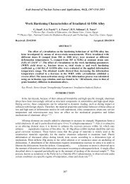
The aim <strong>of</strong> the present experimental work was to study the effect <strong>of</strong> the thermal <strong>and</strong> hydraulic<br />
parameters on the fuel clad integrity <strong>of</strong> an electrically heated test section. This test section simulates a<br />
full square bundle <strong>of</strong> Egypt’s first research reactor (ET-RR1). A schematic diagram <strong>of</strong> the experimental<br />
set up with all its main components is shown in (Fig. 1). It is composed <strong>of</strong> two main loops namely the<br />
primary <strong>and</strong> secondary cooling circuits. In the primary loop, flow is induced in the fuel bundle (test<br />
section) downward through the plenum flange to the pump, through the ball valve, the orifice meter,<br />
the heat exchanger <strong>and</strong> finally to the lower plenum orifice flange where it flows upward in the core<br />
tube <strong>and</strong> back to the test section. In the secondary circuit, flow is induced by the circulating pump to<br />
the cooling tower, to the shell side <strong>of</strong> the heat exchanger <strong>and</strong> back to the pump. The core tube was mad<br />
<strong>of</strong> stainless steel with an inner diameter <strong>of</strong> 142 mm <strong>and</strong> a height <strong>of</strong> 940 mm. A manometer tapping was<br />
drilled at 700 mm from the base <strong>of</strong> the core tube <strong>and</strong> another tapping at about 750 mm from core tube<br />
base was constructed for thermocouples outlets. The coolant entrance <strong>and</strong> exit were located in the<br />
orifice flange (Fig.4) where they were separated by the test section body as shown in (Fig.1). The<br />
power header was constructed above the core tube to facilitate assembling <strong>and</strong> disassembling <strong>of</strong> the<br />
test section <strong>and</strong> its components <strong>and</strong> also to host the D.C. power grid to the heating elements within the<br />
test section. It was made <strong>of</strong> stainless steel tube <strong>of</strong> 148 mm in diameter <strong>and</strong> 185 mm in height.<br />
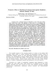
The square bundle consisted <strong>of</strong> the fuel rods, the upper grid <strong>and</strong> the lower grid (Fig.3). A set <strong>of</strong><br />
16 rods <strong>of</strong> 10 mm outer diameter was used to simulate actual fuel rods. One <strong>of</strong> these rods, towards the<br />
center <strong>of</strong> the rod bundle, was instrumented with thermocouples for temperature measurements <strong>and</strong> was<br />
surrounded by 8 heating rods to mimic the ambient heating conditions <strong>of</strong> the instrumented rod. The<br />
other 7 rods were just used to provide the same hydraulic resistance in the actual square fuel bundle.<br />
The heating element (Fig. 2) was made <strong>of</strong> stainless steel <strong>and</strong> was machined to produce a heat<br />
generation function representing a distorted cosine with the maximum heat generation rate towards the<br />
lower half <strong>of</strong> the heating element. Direct electric current was supplied to the test section from a 100<br />
KVA electric power supply. Chromel-Alumel, type K thermocouples were used for temperature<br />
measurements. The thermocouple wires were 0.1 mm in diameter with each <strong>of</strong> its two wires wrapped<br />
with glass wool insulator. Moreover, the thermocouples were completely insulated from the DC power<br />
conducted to the heating rods as well as the cooling water. This was achieved by coating the<br />
thermocouples body <strong>and</strong> the junctions with a thin layer <strong>of</strong> a thermal paint to provide rapid response to<br />
temperature variations. The thermocouples were calibrated using the cold junction method <strong>and</strong> a third<br />
order polynomial was fitted to readily transform the measured voltage to temperature readings. The<br />
clad surface temperature distribution during steady state runes was determined by a set <strong>of</strong> nine<br />
thermocouples impeded at the outer surface <strong>of</strong> the insulator material between the heating element <strong>and</strong><br />
the clad inner surface.<br />
The volumetric flow rate <strong>of</strong> the primary coolant circuit was measured using a st<strong>and</strong>ard<br />
calibrated sharp-edged orifice meter. The orifice plate was located around 110 cm away from the<br />
regulating valve to ensure fully developed flow conditions. Also the orifice meter was calibrated to<br />
relate the measured pressure drop across the orifice plate with the flow rate measurements.<br />
277
<strong>Arab</strong> <strong>Journal</strong> Of <strong>Nuclear</strong> Science And <strong>Applications</strong>, 46(2), (276-286) 2013<br />
Fig.1. A schematic diagram <strong>of</strong> the experimental set up<br />
278
<strong>Arab</strong> <strong>Journal</strong> Of <strong>Nuclear</strong> Science And <strong>Applications</strong>, 46(2), (276-286) 2013<br />
Fig. 2. Lower plenum orifice flange.<br />
Fig. 3. Sectional view <strong>of</strong> the test section.<br />
Fig.4. Sectional view <strong>of</strong> the heating element<br />
279
<strong>Arab</strong> <strong>Journal</strong> Of <strong>Nuclear</strong> Science And <strong>Applications</strong>, 46(2), (276-286) 2013<br />
The data obtained from measuring instruments were collected <strong>and</strong> processed using data<br />
acquisition system. The raw data from measuring transducers are usually <strong>of</strong> low level <strong>and</strong> are thus<br />
prone to distortion. For example, the emf <strong>of</strong> the different thermocouples junctions was found to be<br />
ranging from 0 to 60.84 v/ o c (at 20 o c). A set <strong>of</strong> sequenced operations was introduced to make these<br />
signals amenable for recording in a computer. This includes amplifications, filtration, multiplexing,<br />
conversion to digital signal, demultiplexing, recording <strong>and</strong> finally processing. All these operations<br />
should take place in no time, hypothetically. However, there is indeed some time taken during these<br />
processes <strong>and</strong> if this time is larger than the time it takes for the physical phenomena to change, the<br />
automated measuring system will not be able to catch the actual changes <strong>of</strong> the studied phenomena. It<br />
is thus important to minimize these response times during each <strong>of</strong> the above mentioned processes. All<br />
cautions were taken to achieve this goal including the minimization <strong>of</strong> thermocouple diameter, the<br />
choice <strong>of</strong> a higher rate A\D converter, etc. After assembling the test rig, a cold run was carried out to<br />
check the consistency <strong>of</strong> the operating conditions, measuring devices <strong>and</strong> data acquisition system.<br />
MODELING APROACH<br />
The direct numerical solution <strong>of</strong> the momentum <strong>and</strong> energy equations in such a complex system<br />
which runs at moderately higher Reynolds number may not be attainable with the current available<br />
computing powers. The other alternative may be to adopt the RANS technique in order to make the<br />
system amenable to solution. In the RANS technique, one ab<strong>and</strong>ons the need for comprehensive,<br />
complete details <strong>of</strong> the instantaneous flow field <strong>and</strong> heat transfer, <strong>and</strong> is satisfied with the time<br />
averaged quantities that RANS determines. Albeit the fact that these averaged quantities provides us<br />
with somehow crude approximation to the real variables, they are, in most <strong>of</strong> our engineering<br />
applications, acceptable <strong>and</strong> can provide us with quite satisfying criteria for design purposes. The<br />
problem <strong>of</strong> using RANS approach, however, is that till now, there is no unifying set <strong>of</strong> equation to<br />
model all kinds <strong>of</strong> turbulent flows <strong>and</strong> heat transfer scenarios. The reason for this may be the fact that<br />
performing time averaging <strong>of</strong> the momentum <strong>and</strong> energy equations results in unclosed systems. In<br />
other words, the RANS equations contains terms that are related to the fluctuation components <strong>of</strong> the<br />
corresponding averaged quantities. There exist quite a number <strong>of</strong> models to close the system <strong>of</strong><br />
equations <strong>and</strong> to propose relationships between the averaged fluctuating components <strong>and</strong> the mean<br />
field variables. On the other h<strong>and</strong>, since turbulence models are usually valid in the main flow field,<br />
special care need to be taken should there exist confining walls. The reason for that stems from the<br />
complex structure <strong>of</strong> the boundary layer in the vicinity <strong>of</strong> the confining walls. That is, while the flow<br />
in the main stream may be quite chaotic <strong>and</strong> turbulent, the flow right near to the wall is still laminar<br />
because <strong>of</strong> the viscosity effects. This layer, where viscous effects dominate inertial effects, is called the<br />
laminar sublayer <strong>and</strong> is confined closer to the wall boundaries. Right subsequent to this layer is a layer<br />
called the buffer zone in which a transition from laminar flow to the full turbulent flow is taking place.<br />
It is apparent that turbulence models are not applicable in this two regions <strong>and</strong> hence special treatment<br />
need to be devised. Two approaches are currently available to simulating the near-wall region. In the<br />
first approach, both the viscous sublayer <strong>and</strong> the buffer zone are not resolved <strong>and</strong> semi-empirical<br />
formulas are used to smoothly extend the turbulence models to wall. These formulas are called wallfunctions<br />
<strong>and</strong> they comprise law <strong>of</strong> the wall for mean quantities <strong>and</strong> formulas for near wall turbulent<br />
quantities. In the second approach, on the other h<strong>and</strong>, the turbulence models are modified in such a<br />
way as to be able to resolve the viscosity-affected region. The draw back <strong>of</strong> this approach, however, is<br />
that it requires a very fine mesh in the vicinity <strong>of</strong> the wall including nodes in the viscous sub layer.<br />
1-The choice <strong>of</strong> turbulence model.<br />
As stated earlier, the main focus <strong>of</strong> this research was to study the integrity <strong>of</strong> the clad material<br />
under different operating conditions. Hence, no measurements were taken to evaluate turbulence<br />
quantities (e.g., Reynolds stresses) that may help in suggesting the appropriate turbulence model. It<br />
280
<strong>Arab</strong> <strong>Journal</strong> Of <strong>Nuclear</strong> Science And <strong>Applications</strong>, 46(2), (276-286) 2013<br />
was, thus, important to survey over the available turbulence models in terms <strong>of</strong> their criteria <strong>of</strong><br />
applicability, limitations <strong>and</strong> restrictions in order to choose the one that might be appropriate to model<br />
this complex system. Moreover, literature surveys were conducted to explore on what other researcher<br />
have recommended for similar systems. It was found that substantial amount <strong>of</strong> research work have<br />
been done on rod bundle geometry using the st<strong>and</strong>ard k turbulence models over the past few<br />
decades for a recent in-depth review on CFD analysis on rod bundle geometries ( Tzanos 2001 (1) ). In<br />
general, there is a great deal <strong>of</strong> agreement between researchers that the st<strong>and</strong>ard k model may not<br />
be the turbulence model <strong>of</strong> choice in rod bundle geometries. On the other h<strong>and</strong>, most <strong>of</strong> these<br />
researches have considered periodic arrays <strong>of</strong> rods which allowed them to solving the flow in<br />
elementary sections <strong>and</strong> assuming symmetry across the boundaries (Rapley <strong>and</strong> Gosman 1986 (2) ;<br />
Baglietto <strong>and</strong> Ninokata, 2005 (3) ; <strong>and</strong> many others). However, as Chang <strong>and</strong> Tavoularis, 2007 (4) pointed<br />
out, this approach restricts the solution based on the fact that symmetry in geometrical configurations<br />
does not necessarily imply symmetry in the flow. In other words, simulating a full sector may be<br />
required to better capture the essential features <strong>of</strong> the flow field. It was reported the use <strong>of</strong> the shearstress<br />
transport (SST) k <br />
model to perform CFD analysis <strong>of</strong> flow field in a triangular rod bundle<br />
by Toth <strong>and</strong> Aszodi (2008) (5) . Chang <strong>and</strong> Tavoularis, 2005 (6) , on the other h<strong>and</strong>, used the unsteady<br />
Reynolds averaged Navier-Stokes equations supplemented by a st<strong>and</strong>ard Reynolds stress model to<br />
simulate the experimental work <strong>of</strong> Guellouz <strong>and</strong> Tavoularis 2000 (7) a,b <strong>and</strong> reported good agreement.<br />
In this work, we consider the use <strong>of</strong> the shear-stress transport (SST) <br />
Toth <strong>and</strong> Aszodi, 2008 (5) . Moreover, the two approaches to dealing with the near wall region were<br />
considered with the aim that if it is founded that the wall function approach provides reasonable<br />
approximation to the measured inner clad surface temperature, then it might be recommended for<br />
further investigation since it usually requires less computing resources.<br />
2-The Shear-Stress Transport (SST) <br />
k model<br />
281<br />
k model as suggested by<br />
k <strong>and</strong> SST models, which are basically two equation eddy-viscosity models, the<br />
In both the <br />
Reynolds stresses can be calculated from the eddy-viscosity hypothesis introduced by Boussinesq,<br />
(Pope, 2000 (8) ):<br />
2 <br />
<br />
U<br />
uiu j k<br />
ij <br />
t<br />
3 <br />
<br />
x<br />
j<br />
i<br />
U<br />
<br />
x<br />
i<br />
j<br />
<br />
<br />
<br />
<br />
As suggested by Menter, if it is possible to combine the st<strong>and</strong>ard <br />
shows to be relatively accurate if applied to the near wall region with the <br />
accurate in the far field, one may obtain a model that may be used in a variety <strong>of</strong> applications<br />
involving confining walls. This model is called the shear-stress transport <br />
basically the same formulation as the st<strong>and</strong>ard <br />
activate the <br />
region. In addition the definition <strong>of</strong> turbulent viscosity is modified to account for the transport <strong>of</strong> the<br />
turbulent shear stress.<br />
(1)<br />
k model, Wilcox, which<br />
k model which is also<br />
k model. It has<br />
k model but it includes blending function to<br />
k model in the near-wall region or the transformed <br />
k away from the wall<br />
In this model, the turbulent kinetic energy, k, <strong>and</strong> the specific dissipation rate, , may be<br />
obtained from the following transport equations (FLUENT, 2006 (9) ):<br />
k<br />
~<br />
( k)<br />
( kui<br />
) (<br />
k<br />
) Gk<br />
Yk<br />
S k<br />
(2)<br />
t<br />
xi<br />
x<br />
j <br />
x<br />
j
<strong>Arab</strong> <strong>Journal</strong> Of <strong>Nuclear</strong> Science And <strong>Applications</strong>, 46(2), (276-286) 2013<br />
<br />
<br />
( ) ( u<br />
) <br />
G<br />
Y<br />
D<br />
S<br />
(3)<br />
<br />
<br />
i<br />
<br />
t xi<br />
x<br />
j x<br />
j<br />
where k<br />
G~ represents the generation <strong>of</strong> turbulence kinetic energy due to the mean velocity gradients,<br />
G the generation <strong>of</strong> , k<br />
<strong>and</strong> <br />
Y represents the dissipation <strong>of</strong> k <strong>and</strong> due to turbulence, <br />
S k , S<br />
are source terms.<br />
Now, k<br />
as<br />
<strong>and</strong> <br />
<br />
t<br />
k ,<br />
k<br />
represents effective diffusivity <strong>of</strong> k <strong>and</strong> , k<br />
282<br />
Y <strong>and</strong><br />
D represents the cross-diffusion term, <strong>and</strong><br />
represent the effective diffusivity <strong>of</strong> the k <strong>and</strong> , respectively, which are defined<br />
<br />
t<br />
with k<br />
<br />
<strong>and</strong> <br />
are the turbulent Pr<strong>and</strong>tl numbers <strong>and</strong> that is<br />
where the blending function is used to ensure that the model equations would work in both the nearwall<br />
<strong>and</strong> the far-field regions.<br />
On the other h<strong>and</strong>, the energy equation is modeled analogous to Reynolds treatment to<br />
turbulent momentum transfer. That is the energy equation as modeled in FLUENT takes the form:<br />
<br />
T <br />
E ui<br />
E p <br />
<br />
( ) [ ( )] keff<br />
u <br />
i ( ij ) eff S h<br />
(4)<br />
t<br />
xi<br />
x<br />
<br />
j x <br />
j <br />
k is the effective thermal conductivity, <strong>and</strong> eff<br />
( is the deviatoric<br />
Where E is the total energy, eff<br />
stress tensor. This term represents the irreversible dissipation <strong>of</strong> kinetic energy to heat energy.<br />
Moreover, the unified wall thermal treatment blends the laminar <strong>and</strong> logarithmic pr<strong>of</strong>iles according to<br />
the method <strong>of</strong> Kader (1981 (10) ) in which the convective heat flux is calculated as, (Koncar et al. 2005)<br />
C u<br />
q <br />
L pL W<br />
( TW<br />
T<br />
l,<br />
( nw)<br />
T <br />
y ( L)<br />
Here )<br />
l,<br />
( nw<br />
)<br />
T is the liquid temperature in the near-wall computational cell,<br />
dimensional temperature at the non-dimensional distance from the near-wall cell,<br />
friction velocity.<br />
3-Mesh sensitivity analysis<br />
ij )<br />
<br />
<br />
y (L)<br />
(5)<br />
T is the non-<br />
<br />
y nw <strong>and</strong> w<br />
u is the<br />
In this work we consider two kinds <strong>of</strong> meshes, in the first one both the viscous sublayer <strong>and</strong> the<br />
buffer zone are not resolved <strong>and</strong> hence wall function technique was assumed. Although this meshing<br />
strategy is considered coarse, it is amid at giving a rough estimation on the axial clad temperature<br />
pr<strong>of</strong>ile based on the availability <strong>of</strong> less computing resources. In the other approach, a very fine mesh<br />
in the neighborhood regions <strong>of</strong> heating rods <strong>and</strong> basket wall were assumed. As Toth <strong>and</strong> Aszodi<br />
(2008 (8) <br />
) reported in their work that meshes with average y <strong>of</strong> approximately 1 <strong>and</strong> 20.1 were<br />
acceptable to capturing the basic flow field characteristic. Hence, meshes which are very fine near the<br />
wall may be difficult to implement, particularly for complicated, larger geometries. In this work,<br />
however, we consider a mesh with <br />
opportunity to get accurate estimation <strong>of</strong> the flow field at reasonable cost in terms <strong>of</strong> computing<br />
resources in addition to the fact that, this work is not primarily aiming at examining processes in the<br />
y in the order <strong>of</strong> 5. It is believed that this will also give us the
viscous sub-layer.<br />
<strong>Arab</strong> <strong>Journal</strong> Of <strong>Nuclear</strong> Science And <strong>Applications</strong>, 46(2), (276-286) 2013<br />
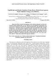
Fig. 5-a,b show cross sectional grids for 45 o -sector <strong>of</strong> the complete rod bundle with Fig.5-a<br />
shows the coarse mesh <strong>and</strong> Fig.5-b represents the finer mesh. Fig. 6, on the other h<strong>and</strong>, shows the 3D<br />
mesh <strong>of</strong> a sectional cut <strong>of</strong> the simulated sector.<br />
RESULT AND DISCUSSION<br />
The steady state simulation was performed on a windows-based personal computer with Intel<br />
Quad dual processor. The commercial CFD code FLUENT 6.2.12, which solves the governing<br />
equations by the finite volume approach, was used for simulation. The convective terms were<br />
discretized using a second-order upwind scheme. The pressure field was coupled to the velocity field<br />
by the SIMPLE algorithm. Also, the energy equation was discretized by a second-order upwind<br />
scheme. Flow convergence was considered achieved when the residuals for all flow variables reaches<br />
lower than 10 -4 . Pressure inlet <strong>and</strong> outlet boundary conditions were set for the inlet <strong>and</strong> outlet sections,<br />
respectively, with the pressure gradient adjusted to match the desired mass flow rate. The side faces,<br />
on the other h<strong>and</strong> were considered symmetry faces. The present simulations were validated by<br />
comparing the measured inner clad surface temperatures with the result <strong>of</strong> simulation. As indicated<br />
earlier, the instrumented rod, which is the one near the centerline <strong>of</strong> the square bundle, was equipped<br />
with a set <strong>of</strong> 8 thermocouples impeded into the insulating material to measure the inner clad surface<br />
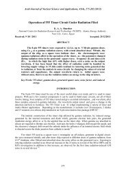
temperature. Temperature contours is shown in Fig 7. It is apparent that the hot spots are almost<br />
towards the lower half <strong>of</strong> the heating elements. Fig. 8, on the other h<strong>and</strong>, shows the comparison<br />
between measured inner clad surface temperatures with that simulated. The simulated, axial-wise<br />
average inner clad temperatures were extracted using a UDF. As the figure shows, quite good<br />
agreement is obtained between measurements <strong>and</strong> simulation which provide confidence in the<br />
modeling approach. It is apparent that the maximum inner clad surface temperature is shifted towards<br />
the center <strong>of</strong> the lower half <strong>of</strong> the heating element following the general trend <strong>of</strong> the heat generation<br />
function adapted to the heating elements. Fig. 9, also, depicts the axial average temperature variations<br />
at the surface <strong>of</strong> the heating element, <strong>and</strong> at the clad inner <strong>and</strong> outer surfaces. One can notice that there<br />
is a very little temperature drop within the clad material because <strong>of</strong> the higher thermal conductivity <strong>of</strong><br />
its material. Velocity vector field at the plane z = 0.125 is shown in Fig. 10. It is apparent that the<br />
maximum velocity is at the middle <strong>of</strong> the gaps between heating rods.<br />
Fig. 5a. cross sectional grids for 45 o -sector<br />
( the coarse mesh )<br />
283<br />
Fig. 5b. cross sectional grids for 45 o -sector (the<br />
finer mesh)
<strong>Arab</strong> <strong>Journal</strong> Of <strong>Nuclear</strong> Science And <strong>Applications</strong>, 46(2), (276-286) 2013<br />
Fig.6. The 3D mesh <strong>of</strong> a sectional cut <strong>of</strong> the<br />
simulated sector.<br />
284<br />
Fig. 7. Temperature contours <strong>of</strong> the inner clad<br />
surface
T emperature, c<br />
<strong>Arab</strong> <strong>Journal</strong> Of <strong>Nuclear</strong> Science And <strong>Applications</strong>, 46(2), (276-286) 2013<br />
160<br />
140<br />
120<br />
100<br />
80<br />
60<br />
40<br />
20<br />
0<br />
P ower 100%<br />
0 0. 1 0. 2 0. 3 0. 4 0. 5 0. 6<br />
Dista nc e from bottom, m<br />
285<br />
Measur ed<br />
SST- Si mul at ed<br />
Fig. 8. The comparison between measured inner clad surface temperatures <strong>and</strong> simulated.<br />
Fig. 9. the axial average temperature variations at the surface <strong>of</strong> the heating element, <strong>and</strong> at the<br />
clad inner <strong>and</strong> outer surfaces
<strong>Arab</strong> <strong>Journal</strong> Of <strong>Nuclear</strong> Science And <strong>Applications</strong>, 46(2), (276-286) 2013<br />
Fig. 10. Velocity vector field at the plane z = 0.125<br />
REFERENCE<br />
k turbulence models in the simulation <strong>of</strong> LWR fuel-bundle<br />
1- Tzanos, C. 2001, Performance <strong>of</strong> <br />
flows, Trans. ANS 84, pp. 197-199.<br />
2- Rapley, C.W., <strong>and</strong> Gosman, A.D., 1986, The prediction <strong>of</strong> fully developed axial turbulent flow in<br />
rod bundles, <strong>Nuclear</strong> Engineering <strong>and</strong> Design, 97, pp. 313-325.<br />
3- Baglietto, E., <strong>and</strong> Ninokata, H., 2005, A turbulence model study for simulating flow inside tight<br />
lattice rod bundles. <strong>Nuclear</strong> Engineering <strong>and</strong> Design, 235, pp. 773-784.<br />
4- Chang, D., <strong>and</strong> Tavoularis, S., 2007, Numerical simulation <strong>of</strong> turbulent flow in a 37- rod bundle,<br />
<strong>Nuclear</strong> Engineering <strong>and</strong> Design, 237, pp 575-590.<br />
5- Toth, S. <strong>and</strong> Aszodi, A., 2008, CFD analysis <strong>of</strong> flow field in a triangular rod bundle, <strong>Nuclear</strong><br />
Engineering <strong>and</strong> Design,<br />
6- Chang, D., <strong>and</strong> Tavoularis, S., 2005, Unsteady numerical Simulation <strong>of</strong> turbulence <strong>and</strong> coherent<br />
structures in axial flow near narrow gap. J. fluid Engineering, 127, pp 458-466.<br />
7- Guellouz. M, <strong>and</strong> Tavoularis, S., 2000, The structure <strong>of</strong> turbulent flow in rectangular channel<br />
contaning a cylindrical rod- part 1. Renolds averaged measurements, Exp. Thermal fluids, 23, pp 59-<br />
73.<br />
8- Pope, S., 2000, Turbulent flows, Cambridge university pres.<br />
9- Chang, D., <strong>and</strong> Tavoularis, S., 2008, Simulation <strong>of</strong> turbulence, heat transfer <strong>and</strong> mixing across<br />
narrow gaps between rod-bundle subchannel, <strong>Nuclear</strong> Engineering <strong>and</strong> Design, 238, pp 109-123.<br />
10- Kader, B.A., 1981, Temperature <strong>and</strong> concentration pr<strong>of</strong>iles in fully turbulent boundary layers, Int.<br />
J. Heat Mass Transfer 24, 1541-1544.<br />
286