Download - Arab Journal of Nuclear Sciences and Applications

Arab Journal of Nuclear Science and Applications, 46(1), (359-373) 2013 

On Selection of the Probability Distribution for Representing the Maximum 

Annual Wind Speed in East Cairo, Egypt 

Gh. I. El-Shanshoury and S. T. El-Hemamy 

The Nuclear and Radiological Control Authority, Cairo, Egypt 

Received: 25/3/2012 Accepted: 6/6/2012 

ABSTRACT 

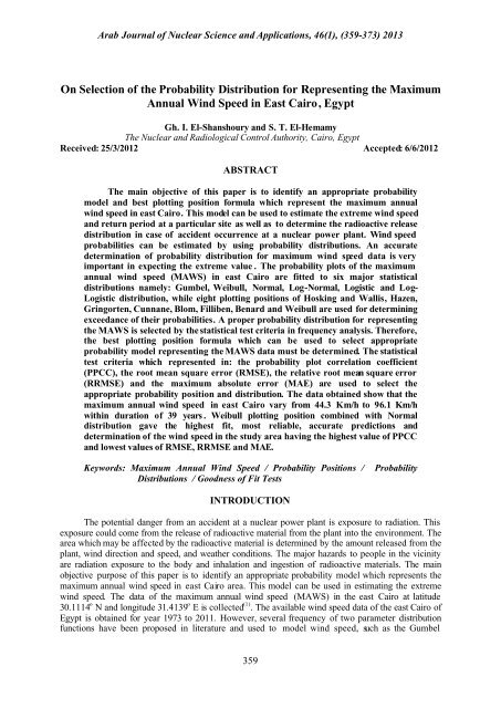
The main objective of this paper is to identify an appropriate probability 

model and best plotting position formula which represent the maximum annual 

wind speed in east Cairo. This model can be used to estimate the extreme wind speed 

and return period at a particular site as well as to determine the radioactive release 

distribution in case of accident occurrence at a nuclear power plant. Wind speed 

probabilities can be estimated by using probability distributions. An accurate 

determination of probability distribution for maximum wind speed data is very 

important in expecting the extreme value . The probability plots of the maximum 

annual wind speed (MAWS) in east Cairo are fitted to six major statistical 

distributions namely: Gumbel, Weibull, Normal, Log-Normal, Logistic and Log- 

Logistic distribution, while eight plotting positions of Hosking and Wallis, Hazen, 

Gringorten, Cunnane, Blom, Filliben, Benard and Weibull are used for determining 

exceedance of their probabilities. A proper probability distribution for representing 

the MAWS is selected by the statistical test criteria in frequency analysis. Therefore, 

the best plotting position formula which can be used to select appropriate 

probability model representing the MAWS data must be determined. The statistical 

test criteria which represented in: the probability plot correlation coefficient 

(PPCC), the root mean square error (RMSE), the relative root mean square error 

(RRMSE) and the maximum absolute error (MAE) are used to select the 

appropriate probability position and distribution. The data obtained show that the 

maximum annual wind speed in east Cairo vary from 44.3 Km/h to 96.1 Km/h 

within duration of 39 years . Weibull plotting position combined with Normal 

distribution gave the highest fit, most reliable, accurate predictions and 

determination of the wind speed in the study area having the highest value of PPCC 

and lowest values of RMSE, RRMSE and MAE. 

Keywords: Maximum Annual Wind Speed / Probability Positions / Probability 

Distributions / Goodness of Fit Tests 

INTRODUCTION 

The potential danger from an accident at a nuclear power plant is exposure to radiation. This 

exposure could come from the release of radioactive material from the plant into the environment. The 

area which may be affected by the radioactive material is determined by the amount released from the 

plant, wind direction and speed, and weather conditions. The major hazards to people in the vicinity 

are radiation exposure to the body and inhalation and ingestion of radioactive materials. The main 

objective purpose of this paper is to identify an appropriate probability model which represents the 

maximum annual wind speed in east Cairo area. This model can be used in estimating the extreme 

wind speed. The data of the maximum annual wind speed (MAWS) in the east Cairo at latitude 

30.1114 o N and longitude 31.4139 o E is collected (1) . The available wind speed data of the east Cairo of 

Egypt is obtained for year 1973 to 2011. However, several frequency of two parameter distribution 

functions have been proposed in literature and used to model wind speed, such as the Gumbel 

359


distribution ( 2-6) , the Weibull distribution (5-9) , the Log-Normal distribution (9,10) and the Normal 

distribution (11) , the Logistic distribution (12) and the Log-Logistic distribution (10,13) . Moreover, There are 

several plotting position formulas are used for estimating the exceedance probability function such as 

Weibull (2,14,15,1616,21) , Gringorten (17-21) , Hazen (18,21) , Cunnane (18-20) , Blom (18-21) , Benard (18,21) , Filliben (22) as 

well as Hosking and Wallis (23) . The study is based on selecting the best probability plotting position 

and an appropriate probability distribution representing the data. Eight formulas of probability position 

namely: Hosking and Wallis (24) , Hazen (25) , Gringorten (26) , Cunnane (27) , Blom (28) , Filliben (29) , Benard (30) 

and Weibull (31) are compared to choose the best one that can be used for constructing some distribution 

probability plots. Six theoretical probability distributions are compared to present the more appropriate 

model for representing the MAWS in east Cairo. More specifically, the six probability models which 

have two parameters, are the Gumbel (extreme value type I (EVI)), the Weibull, the Normal, the Log- 

Normal, the Logistic and the Log-Logistic distribution. The performance of different probability 

positions and distributions is compared using four statistical test criteria. Many researchers used the 

goodness of fit test criteria for measuring the performance of statistical probability distributions such 

as root mean square error (RMSE) (18,32) , relative root mean square error (RRMSE) (20,32) , maximum 

absolute error (MAE) (32) probability plot correlation coefficient (PPCC) (20, 32, 33, 34) and coefficient of 

determination (R 2 ) (18, 33) . 

In this work, the probability plot correlation coefficient (PPCC), the root mean square error 

(RMSE), the relative root mean square error (RRMSE) and the maximum absolute error (MAE) are 

calculated. The results show that, the Weibull plotting position combined with the Normal distribution 

gave the highest fit, most reliable and accurate predictions of the wind speed in the study area having 

the highest value of PPCC and lowest values of RMSE, RRMSE and MAE. 

1. Probability distributions 

METHODOLOGY 

Several probability models have been developed to describe the distribution of annual extreme 

wind speed at a single site. However, the choice of a suitable probability model is still one of the 

major problems in engineering practice. The selection of an appropriate probability model depends 

mainly on the characteristics of available wind speed data at the particular site. Hence, it is necessary 

to evaluate many available distributions in order to find a suitable model that could provide accurate 

extreme wind speed estimates. Therefore, the main objective of the present study is to propose a 

general procedure for evaluating systematically the performance of various distributions. Six 

probability distributions are investigated, namely: Gumbel (extreme value type I (EVI)), Weibull, 

Normal, Log-Normal, Logistic and Log-Logistic distribution. The probability density function (PDF) f 

(x) and cumulative distribution function (CDF) F(x) and the associated parameters for each of 

probability distribution are: 

Gumbel (EVI) distribution: 

f ( x) = (1/ σ)exp{ −( x−μ)/ σ −exp[ −( x− 

μ)/ σ]} 

, −∞ ≺ x ≺ ∞ 

(1) 

F( x) = exp{ − exp[ −( x− μ)/ σ]} 

(2) 

f(x) is the PDF, F(x) is the CDF, μ is the location parameter and σ is the scale paeameter . 

Weibull distribution: 

f ( x) = σ 

−λ λx λ−1 exp{ − ( x / σ) 

λ 

} , 0 ≤ x, 0 ≺ σλ , 

(3) 

F( x) = 1−exp{ − ( x/ 

σ ) 

λ 

} 

(4) 

360


f(x) is the PDF, F(x) is the CDF, σ is the scale parameter and λ is the shape parameter . 

Normal distribution: 

f ( x) = 1 exp{ −1 [( )/ ]} 

2 

2 

2 

x− μ σ , −∞ ≺ x ≺ ∞ 

(5) 

σ π 

F( x) =Φ[( x− μ)/ σ] 

(6) 

standardized from: μ=0, σ=1 where, Φ is CDF of standard Normal (0,1) distribution . 

μ is the location parameter and σ is the scale parameter. 

Log-Normal distribution: 

f ( x) = 1 exp{ − 1 [(ln 

2 

2 

x− 

μln x)/ σlnx] 

} , 0 ≺ x 

(7) 

xσ 

2π 

lnx 

F( x) =Φ[(ln x− μlnx)/ σ ln x] 

(8) 

standardized from: μ=0, σ=1 where, Φ is CDF of standard Normal (0,1) distribution . 

μ is the scale parameter and σ is the shape parameter. 

Logistic distribution: 

f ( x) 

= 

exp{( x − μ)/ σ} 

σ[1+ exp{( x −μ)/ 

σ}] 

2 , −∞≺ x ≺ ∞ 

(9) 

F( x) 

= 

exp{( x − μ)/ σ} 

(10) 

1 + exp{( x −μ)/ 

σ} 

μ is the location parameter and σ is the scale parameter. 

Log-Logistic distribution: 

f ( x) 

= 

exp{(ln x − μ)/ σ} 

σx[1+ exp{(ln x−μ)/ 

σ}] 

2 , 0 ≺x≺ ∞ 

(11) 

F( x) 

= 


1 + exp{(ln x −μ)/ 

σ} 

μ is the scale parameter and σ is the shape parameter. 

2. Plotting positions 

Many empirical formulas have been proposed for the determination of plotting positions. Most 

of them can be expressed generally in the following form: 

ˆ F (x≥ xT)= (i-a)/(n+1-2a) (13) 

or in a general form: 

ˆ F ( x≥ xT)=(i-a)/(n+b) (14) 

where: ˆ F is the exceedance probability of extreme value, 

xT is the extreme probable value, 

a is a constant. 

The existing plotting position formula in form of Eq. (13): a is equal to 0.5 for Hazen's formula; 

zero for Weibull's formula; 3/8 for Blom's formula; 0.44 for Gringorten's formula; 0.3 for Benard's 

formula; 0.4 for Cunnane's formula and 0.3175 for Filliben's formula. 

The existing plotting position formula in form of Eq. (14): a is equal to 0.35 and b is equal to 

0.0 for Hosking and Wallis. These plotting position formulas are listed in Table 1. The common 

technique of these formulas is to arrange the observed data in descending order of magnitude and 

assign an order number (i) to the rank value. Then the probability ( ˆ F ) of each event being exceeded is 

determined using plotting position formula (21) . 

361 

(12)


Table (1): plotting position formulas 

Name Source Relationship (Fi) 

Hosking and Wallis Hosking and Wallis (i-0.35)/n 

Hazen Hazen (i-0.5)/n 

Gringorten Gringorten (i-0.44)/(n+0.12) 

Cunnane Cunnane (i-0.4)/(n+0.2) 

Blom Blom (i-0.375)/(n+0.25) 

Filliben Filliben (i-0.3175)/(n+0.365) 

Benard Benard (i-0.3)/(n+0.4) 

Weibull Weibull i/(n+1) 

3. Probability plot 

The probability plot is a graphical technique for assessing whether or not a data set follows a 

given distribution. The data are plotted against a theoretical distribution in such a way that the points 

should form approximately a straight line. The estimates of the two parameters of distributions can be 

found graphically using the probability plot. The correlation coefficient (PPCC) associated with the 

linear fit to the data in the probability plot is a measure of the goodness of the fit. Estimates of 

the location and scale parameters of the distribution are given by the intercept and slope. Probability 

plots can be generated for several competing distributions to see which provides the best fit, and the 

probability plot generating the highest correlation coefficient is the best choice since it generates the 

straightest probability plot. 

To construct the probability plot the observed data xi are ranked in ascending order, and denoted 

from x1:n to xn:n, where n is the total number of observations. A plotting position of the non-exceedance 

probability : 

ˆ F in is computed for each xi:n using some formulas of plotting positions. Parameters for the 

compared distributions are computed using the regression scheme. The regression (graphical) method 

starts with the data in levels, xi or logs, lnxi. Let Fˆ i is probability position. The horizontal axis (g ( F ˆ 

i )) 

is a transformation of F ˆ 

i (the reduce variate). The slope and intercept (denoted a and b), in the 

relationship between g( F ˆ 

i ) and xi (in levels or logs), correspond to the parameters of the model. The 

quantiles function of the distributions is given by: 

xp = a g ( F ˆ 

i ) +b (15) 

Lnxp = a g( F ˆ 

i ) +b (16) 

where xp (expected wind speed) is the quantiles function of the distributions. 

The correlation coefficient (PPCC) measures the strength of a linear relationship between two 

variables. Hence the correlation of xpi and g( ˆ i 

F ) might be a good way to measure how well each 

distribution fits the data. Table 2 shows the coordinates of X-axis and Y-axis of linear relationships 

(probability plots) of the compared probability distributions. 

362


Table (2): the coordinates of X-axis and Y-axis of distributions probability plots 

Model Equation of Cumulative distribution function 

(CDF) 

Gumbel 

(EVI) 

Weibull 

363 

X-axis 

Reduce variate 

(g( F ˆ 

i )) 

F( x) = exp{ −exp[ −( x − μ)/ σ]} 

-ln[-ln( F ˆ 

i )] 

F( x) = 1−exp{ − ( x / σ ) 

λ 

} 

Normal F( x) =Φ[( x − μ)/ σ] 

ln[-ln(1-F ˆ 

i )] 

Φ -1 ( F ˆ 

i ) 

Log- 

Normal 

F( x) =Φ[(ln x − μ)/ σ] 

Φ -1 ( F ˆ 

i ) 

Logistic 

F( x) 

= 

exp{( x − μ)/ σ} 

1 + exp{( x −μ)/ 

σ} 

Log- 

Logistic 

F( x) 

= 


1 + exp{(ln x −μ)/ 

σ} 

ln[Fi/(1-F ˆ 

i )] 

ln[Fi/(1-F ˆ 

i )] 

Where, F - 1 ( ) denotes the inverse standard Normal cumulative distribution function. 

4. Goodness of fit tests 

Y- axis 

xi values 

lnxi values 

xi values 

lnxi values 

xi values 

lnxi values 

It is very important to select an appropriate probability distribution in frequency analysis for the 

estimation of design quantile. An appropriate probability distribution and positions is selected 

generally based on the goodness of fit tests which is the method for examining the fitness between 

sample data and its population for a given probability distribution. For ease of computation, four test 

criteria are used. 

The root mean square error (RMSE) also known as the standard error is the sum of squares of the 

differences between observed and computed values: 

RMSE = [(xi – xpi ) 2 /(n -m)] 1/2 (17) 

Where: xi, i =1,…,n are the observed values, 

xpi, i = 1,…,n are the expected values computed from an assumed empirical probability 

distribution using plotting position formula based on the sorted ranks of observed values 

and the number of parameters estimated for the assumed distribution, denoted as m. 

The relative root mean square error (RRMSE) is defined as: 

RRMSE ={S[(xi- xpi ) / xi] 2 /(n- m)} 1/2 (18) 

The maximum abs olute error (MAE) is closely related to the Kolmogorov-Smirnov statistics and 

represents the largest absolute difference between the observed and computed values: 

MAE = max(|xi – xpi |) (19) 

Probability plot correlation coefficient (PPCC) 

PPCC associated with the linear fit to the data in the probability plot. The adequacy of a fitted 

probability position and distribution can be evaluated by the PPCC which is essentially a measure of


the linearity of the probability plot (29) . The probability plot correlation coefficient (PPCC) test has been 

known as powerful and easy test among the goodness of fit tests. The test uses the correlation between 

the ordered observations and the corresponding fitted quantilies, determined by plotting position 

for each xi. 

The PPCC of the fitted distribution at is given by: 

F ˆ 

i 

PPCC = S[(xi - x )( xpi - x pi )]/ [S(xi - x ) 2 S(xpi - x pi ) 2 ] 1/2 (20) 

Where x and x pi denote the average value of the observations and fitted quantiles, respectively (32) . 

RESULTS AND DISCUSSIONS 

This study is carried out on annual extreme wind speed of Cairo airport from year 1973 to 2011 

which is collected from east Cairo. The largest values of annual wind speeds recorded in east Cairo are 

shown in time series given in Figure (1). The highest wind speed of 96.1Km/h was observed in 

1985 and declined to 44.3Km/h in the year 2002. 

Maximum Annual Wind Speed (MAWS),Km/h 

120 

100 

80 

60 

40 

20 

MAWS 

0 

1970 1975 1980 1985 1990 1995 2000 2005 2010 2015 

years 

Fig.(1) Maximum Annual Winds Speed in Cairo Airport, Km/h 

The maximum annual wind speeds are fitted to the Gumbel, Weibull, Normal, Log-Normal, 

Logistic and Log-Logistic distributions and the non-exceedance probabilities determined using the 

various plotting positions formula in Table 2. The determined probabilities of non-exceedance of 

the MAWS ( F ˆ 

i ) before subjecting them to the statistical distributions are shown in Table 3. 

364


Table (3): the probability ( F ˆ 

i ) of each event being not exceeded is determined using plotting 

years 

MAWS 

Km/h 

position formulas 

Hosking and 

Wallis Hazen Gringorten Cunnane Blom Filliben Benard Weibull 

2002 44.3 0.016667 0.012821 0.014315 0.015306 0.015924 0.017338 0.017766 0.025 

2005 46.5 0.042308 0.038462 0.039877 0.040816 0.041401 0.042741 0.043147 0.05 

1976 51.9 0.067949 0.064103 0.06544 0.066327 0.066879 0.068144 0.068528 0.075 

2004 53.5 0.09359 0.089744 0.091002 0.091837 0.092357 0.093548 0.093909 0.1 

1980 55.4 0.119231 0.115385 0.116564 0.117347 0.117834 0.118951 0.119289 0.125 

1981 57.2 0.144872 0.141026 0.142127 0.142857 0.143312 0.144354 0.14467 0.15 

1987 57.2 0.170513 0.166667 0.167689 0.168367 0.16879 0.169757 0.170051 0.175 

1978 59.1 0.196154 0.192308 0.193252 0.193878 0.194268 0.195161 0.195431 0.2 

2007 59.4 0.221795 0.217949 0.218814 0.219388 0.219745 0.220564 0.220812 0.225 

1983 60.7 0.247436 0.24359 0.244376 0.244898 0.245223 0.245967 0.246193 0.25 

1973 61.1 0.273077 0.269231 0.269939 0.270408 0.270701 0.271371 0.271574 0.275 

1975 61.1 0.298718 0.294872 0.295501 0.295918 0.296178 0.296774 0.296954 0.3 

1982 61.1 0.324359 0.320513 0.321063 0.321429 0.321656 0.322177 0.322335 0.325 

2003 61.1 0.35 0.346154 0.346626 0.346939 0.347134 0.34758 0.347716 0.35 

1998 63 0.375641 0.371795 0.372188 0.372449 0.372611 0.372984 0.373096 0.375 

1992 66.5 0.401282 0.397436 0.397751 0.397959 0.398089 0.398387 0.398477 0.4 

2000 72 0.426923 0.423077 0.423313 0.423469 0.423567 0.42379 0.423858 0.425 

1993 73.7 0.452564 0.448718 0.448875 0.44898 0.449045 0.449193 0.449239 0.45 

1974 74.1 0.478205 0.474359 0.474438 0.47449 0.474522 0.474597 0.474619 0.475 

1996 74.1 0.503846 0.5 0.5 0.5 0.5 0.5 0.5 0.5 

1999 74.1 0.529487 0.525641 0.525562 0.52551 0.525478 0.525403 0.525381 0.525 

1989 75.9 0.555128 0.551282 0.551125 0.55102 0.550955 0.550807 0.550761 0.55 

1994 75.9 0.580769 0.576923 0.576687 0.576531 0.576433 0.57621 0.576142 0.575 

2001 75.9 0.60641 0.602564 0.602249 0.602041 0.601911 0.601613 0.601523 0.6 

1984 77.8 0.632051 0.628205 0.627812 0.627551 0.627389 0.627016 0.626904 0.625 

1986 77.8 0.657692 0.653846 0.653374 0.653061 0.652866 0.65242 0.652284 0.65 

1991 77.8 0.683333 0.679487 0.678937 0.678571 0.678344 0.677823 0.677665 0.675 

2010 77.8 0.708974 0.705128 0.704499 0.704082 0.703822 0.703226 0.703046 0.7 

2011 77.8 0.734615 0.730769 0.730061 0.729592 0.729299 0.728629 0.728426 0.725 

1988 79.5 0.760256 0.75641 0.755624 0.755102 0.754777 0.754033 0.753807 0.75 

1990 79.5 0.785897 0.782051 0.781186 0.780612 0.780255 0.779436 0.779188 0.775 

2009 79.5 0.811538 0.807692 0.806748 0.806122 0.805732 0.804839 0.804569 0.8 

1977 81.7 0.837179 0.833333 0.832311 0.831633 0.83121 0.830243 0.829949 0.825 

1997 84.8 0.862821 0.858974 0.857873 0.857143 0.856688 0.855646 0.85533 0.85 

2006 87 0.888462 0.884615 0.883436 0.882653 0.882166 0.881049 0.880711 0.875 

2008 88.9 0.914103 0.910256 0.908998 0.908163 0.907643 0.906452 0.906091 0.9 

1979 92.4 0.939744 0.935897 0.93456 0.933673 0.933121 0.931856 0.931472 0.925 

1995 94.3 0.965385 0.961538 0.960123 0.959184 0.958599 0.957259 0.956853 0.95 

1985 96.1 0.991026 0.987179 0.985685 0.984694 0.984076 0.982662 0.982234 0.975 

Probability plot is a graphical technique for assessing whether or not a data set follows a given 

distribution. The data are ranked according to 8 probability positions. The ranked data are evaluated 

with 6 methods of probability distribution functions. Probability plot is constructed according to Table 

2 by using Table 3. 

365


To construct a probability plot, the sample order statistic xi or ln xi is plotted (usually on the vertical axis) against g( F ˆ ) (usually on the 

i 

horizontal axis). The mathematical expressions obtained for various probability distributions at different formulas of plotting position are 

presented in Table 4. The mathematical expressions represent the expected extreme wind speed in the east Cairo. The equations are obtained from 

48 constructing probability plots. 

Table (4): mathematical expressions (predicted values) for various probability distributions at different formulas of probability position 

Probability 

Position 

Gumbel Weibull Normal Log-Normal Logistic Log-Logistic 

Hosking 

and Wallis 

xp = 

9.5674g( F ˆ )+65.224 

i 

Ln(xp)= 

0.1532g( F ˆ )+4.3277 

i 

xp = 

12.909 g( F ˆ )+70.69 

i 

Ln(xp)= 

0.1876g( F ˆ )+ 4.2407 

i 

xp = 

7.169 g( F ˆ )+70.648 

i 

Ln(xp)= 

0.1042 g( F ˆ )+ 4.2401 

i 

Hazen xp = 

Ln(xp) = 

xp = 

Ln(xp)= 

xp = 

Ln(xp )= 

F )+65.304 F )+4.3299 F )+70.96 F )+4.2446 F )+70.96 F )+4.2446 

Gringorten 

Cunnane 

Blom 

Filliben 

9.9286g( ˆ i 

xp = 

10.074 ( ˆ F i )+65.261 

xp = 

10.166g( F ˆ )+65.235 

i 

xp = 

Benard xp = 

Weibull 

10.221g( ˆ i 

xp = 

F )+65.219 

10.344g( ˆ F i )+65.185 

10.38g( F ˆ )+65.174 

i 

xp = 

10.939g( ˆ F i )+65.021 

0.1496g( ˆ i 

Ln( xp)= 

0.1517g( ˆ F i )+4.3305 

Ln( xp)= 

0.153g( F ˆ )+ 4.3308 

i 

Ln( xp)= 

F )+4.3311 

0.1538g( ˆ i 

Ln( xp)= 

0.1556g( ˆ F i )+4.3315 

Ln(xp)= 

0.1561g( ˆ i 

F )+4.3317 

Ln( xp)= 

F )+4.3338 

0.1641g( ˆ i 

12.953 g( ˆ i 

xp = 

13.082 g( ˆ F i )+70.96 

xp = 

13.165 g( F ˆ )+70.96 

i 

xp = 

13.215 g( ˆ i 

xp = 

F )+7 0.96 

13.327 g( ˆ F i )+70.96 

xp = 

13.36 g( F ˆ )+70.96 

i 

xp = 

Selection of Probability Distributions and plotting Positions 

13.887 g( ˆ F i )+70.96 

366 

0.1887g ( ˆ i 

Ln(xp)= 

0.1906g ( ˆ F i )+4.2446 

Ln(xp)= 

0.1918g( ˆ i 

F )+ 4.2446 

Ln( xp)= 

F )+ 4.2446 

0.1925g( ˆ i 

Ln(xp)= 

0.1941g ( ˆ F i )+4.2446 

Ln(xp)= 

0.1946g ( F ˆ )+ 4.2446 

i 

Ln(xp)= 

0.2022g ( ˆ i 

F )+ 4.2446 

7.2155 g( ˆ i 

xp = 

7.3185 g( ˆ F i )+70.96 

xp = 

7.3836 g( F ˆ )+70.96 

i 

xp = 

7.423 g( ˆ i 

xp = 

F )+70.962 

7.5103g( ˆ F i )+70.96 

xp = 

7.5361 g( F ˆ )+70.96 

i 

xp = 

7.934 g( ˆ F i )+70.962 

0.1052 g( ˆ i 

Ln(xp)= 

0.1067 g( ˆ F i )+ 4.2446 

Ln(xp)= 

0.1077 g( F ˆ )+ 4.2446 

i 

Ln(xp)= 

0.1082 g( ˆ i 

Ln(xp)= 

F )+4.2446 

0.1095 g( ˆ F i )+ 4.2446 

Ln(xp)= 

0.1099 g( F ˆ )+ 4.2446 

i 

Ln(xp)= 

0.1156 g( ˆ i 

F )+ 4.2446 

The selection of an appropriate plotting plot formula for each statistical distribution is the most important step that is generally chosen by 

using the goodness of fit tests. The PPCC test is a goodness-of-fit test which measures and evaluates the linearity of the probability plot.


Comparison between eight formulas of plotting position for six probability distributions is done 

to choose the best plotting position and the appropriate probability distribution. The comparison is 

based on four test criteria namely: probability plot correlation coefficient (PPCC), root mean square 

error (RMSE), relative root mean square error (RRMSE) and maximum absolute error (MAE). Table 5 

shows the PPCC, RMSE, RRMSE and MAE between observed and expected values for all compared 

distributions using different formula of plotting positions. The best distribution and plotting position is 

determined according to the highest PPCC and the lowest RRMSE and MAE between observed and 

expected values. It is found that the Normal distribution has the maximum value of PPCC and the 

minimum values of RMSE, RRMSE and MAE of MAWS under each plotting position when it is 

compared with other distributions. Moreover, The Weibull plotting position has the highest value of 

PPCC and the lowest values of RMSE, RRMSE and MAE under each probability distribution when it 

is compared with other plotting positions. 

The results show that the Weibull' plotting position at each distribution has slightly, highest 

value of PPCC and lowest value RMSE, RRMSE and MAE comparing with Benard and Filliben 

plotting position at the same distribution. Then, The Weibull plotting is considered the best formula 

for selection an appropriate distribution, followed by Benard and Filliben, respectively. However, the 

Hosking and Wallis plotting position at Weibull distribution is occupy third rank after Benard plotting 

position. The appropriate probability distribution which representing and excpecing the (MAWS) in 

east Cairo is Normal distribution followed by Weibull and Logistic distribution, respectively. The 

results of Table 5 indicate that the Weibull plotting position combined with Normal distribution give 

the highest fit, most reliable and accurate predictions of the MAWS east Cairo. 

Table (5): The test criteria of different formulas of plotting position for the six compared 

distributions 

Gumbel PPCC RMSE RRMSE MAE 

Weibull 

Weibull 0.962428 3.60902 0.054804 9.135469 

Benard 0.957892 3.816265 0.057238 10.81708 

Filliben 0.957542 3.831737 0.057423 10.93825 

Blom 0.956298 3.886239 0.058073 11.35156 

Cunnane 0.955706 3.911886 0.05838 11.54552 

Gringorten 0.954684 3.955737 0.058909 11.86722 

Hazen 0.952946 4.029084 0.059803 12.39603 

Hosking and Wallis 0.944557 4.364136 0.065102 14.17574 

Weibull 0.984423 2.317373 0.03461 5.293756 

Benard 0.982095 2.424945 0.036981 5.517268 

Filliben 0.981898 2.433873 0.037166 5.527232 

Blom 0.981181 2.466554 0.037854 5.586213 

Cunnane 0.980831 2.482686 0.038175 5.604537 

Gringorten 0.980214 2.50961 0.038741 5.647132 

Hazen 0.979134 2.557409 0.039703 5.709897 


367


Normal 

LogNormal 

Logistic 

Log-Logistic 

Weibull 0.985993 2.216801 0.031988 4.511053 

Benard 0.985354 2.266427 0.032875 4.631627 

Filliben 0.985294 2.271039 0.032958 4.639662 

Blom 0.98507 2.288139 0.033268 4.667573 

Cunnane 0.984958 2.296624 0.033422 4.680275 

Gringorten 0.984758 2.311737 0.033697 4.701851 

Hazen 0.984399 2.338602 0.034187 4.736169 


Weibull 0.978748 2.89681 0.039802 7.538043 

Benard 0.978418 2.980874 0.040164 8.872035 

Filliben 0.97838 2.987394 0.040205 8.963377 

Blom 0.978232 3.012716 0.040364 9.300471 

Cunnane 0.978156 3.025267 0.040447 9.460694 

Gringorten 0.978015 3.046048 0.040597 9.719689 

Hazen 0.977754 3.081486 0.040874 10.14033 


Weibull 0.983891 2.376082 0.035028 4.950543 

Benard 0.981308 2.557818 0.03816 5.100711 

Filliben 0.981113 2.570999 0.038394 5.183935 

Blom 0.980404 2.618351 0.039236 5.473735 

Cunnane 0.980058 2.641093 0.03964 5.607886 

Gringorten 0.979451 2.680602 0.040341 5.834141 

Hazen 0.978389 2.748265 0.041538 6.204728 


Weibull 0.977122 3.145717 0.041462 10.39603 

Benard 0.975251 3.34553 0.043335 12.27261 

Filliben 0.975088 3.360003 0.043492 12.39381 

Blom 0.974492 3.41391 0.044068 12.84099 

Cunnane 0.974199 3.443002 0.044352 13.088 

Gringorten 0.97368 3.486268 0.044841 13.42557 

Hazen 0.972763 3.563297 0.045696 14.01974 


368


Conseqently, the mathematical expression which can be used for expecting the extreme wind 

speed in east Cairo is: 

xp = 13.887 g( ˆ F i )+70.96 

Graphical techniques can be used to visually assess the adequacy of a fitted distribution. The 

probability plots of the six compared distributions using Weibull probability position are shown in 

Figure 2. The Q-Q plots of the compared distributions using Weibull probability position are shown in 

Figure 3. From the Q-Q plot it is obvious that the Normal distribution presenting the best fit for 

MAWS data followed by the Weibull distribution. 

MAWS 

120 

110 

100 

90 

80 

70 

MAWS 

60 

50 

40 

30 

20 

10 

0 

y = 10.939x + 65.021 

-2.0 -1.0 0.0 1.0 2.0 3.0 4.0 

Reduce Variate, Gumbel Distribution 

LN (MAWS) 

369 

LN (MAWS) 

y = 0.1641x + 4.3338 

4.5 

3.5 

2.5 

1.5 

0.5 

0 

-4.0 -3.0 -2.0 -1.0 0.0 1.0 2.0 

Reduce Variate, Weibull Distribution 

5 

4 

3 

2 

1

MAWS 

MAWS 


MAWS 

110 

100 

90 

80 

70 

60 

50 

40 

30 

20 

10 

y = 13.887x + 70.962 

0 

-3.0 -2.0 -1.0 0.0 1.0 2.0 3.0 

Reduce Variate, Normall Distributionll 

MAWS 

110 

100 

90 

80 

70 

60 

50 

40 

30 

20 

10 

y = 7.934x + 70.962 

0 

-5.0 -4.0 -3.0 -2.0 -1.0 0.0 1.0 2.0 3.0 4.0 5.0 

Reduce Variate, Logistic Distribution 

LN (MAWS) 

LN(MAWS) 

370 

LN (MAWS) 

5 

4.5 

4 

3.5 

3 

2.5 

2 

1.5 

1 

0.5 

y = 0.2022x + 4.2446 

0 

-3.0 -2.0 -1.0 0.0 1.0 2.0 3.0 

Reduce Variate, Log-Normal Distribution 

LN (MAWS) 

5 

4.5 

4 

3.5 

3 

2.5 

2 

1.5 

1 

0.5 

y = 0.1156x + 4.2446 

0 

-5.0 -4.0 -3.0 -2.0 -1.0 0.0 1.0 2.0 3.0 4.0 5.0 

Reduce Variate, Log-Logistic Distribution 

Figure (2) The probability plots of compared distributions using Weibull probability position 

Quantile 

120 

100 

80 

60 

40 

20 

Q -Q plot of Gumbel distribution 

Quantile 

0 

40 50 60 70 80 90 100 

MAWS 

Quantile 

100 

80 

60 

40 

20 

Q-Q plot of Weibull distribution 

Quantil 

0 

40 50 60 70 80 90 100 

MAWS

Quantile 

Quantile 

120 

100 

80 

60 

40 

20 

0 

120 

100 

80 

60 

40 

20 


Q-Q plot of Normal distribution 

Quantile 

40 50 60 70 80 90 100 

0 

MAWS 

Q-Q plot of Logistic distribtion 

Quantile 

40 50 60 70 80 90 100 

MAWS 

Quantile 

120 

100 

80 

60 

40 

20 

371 

0 

Quantile 

Q-Q plot of Log-Normal distribution 

Quantile 

40 50 60 70 80 90 100 

120 

100 

80 

60 

40 

20 

0 

MAWS 

Q-Q plot of Log-Logistic distribution 

Quantile 

40 50 60 70 80 90 100 

MAWS 

Figure (3) The Q-Q plots of compared distributions using Weibull probability position 

CONCLUSION 

In this study, the maximum annual wind speed (MAWS) is plotted against their hydrologic 

years. Six probability distributions and eight plotting positions are compared. Fourty eight probability 

plots are constructed to represent the expected extreme wind speed and choose the best distribution 

represents the MAWS in the east Cairo. The performances of the probability distributions are assessed 

using the probability plot correlation coefficient (PPCC), the root mean square error (RMSE), the 

relative root mean square error (RRMSE) and maximum absolute error (MAE). The results proved 

that the Weibull plotting position is considered the best probability position which can be used for 

selecting the appropriate distribution for representing and expecting the MAWS in the east Cairo. The 

best probability positions which followed Weibull plotting position are Benard and Filliben, 

respectively. The appropriate probability distribution model which representing and expecting the 

MAWS in east Cairo is the Normal distribution followed by Weibull and Logistic distribution,


respectively. Then, Weibull plotting position combined with Normal distribution gave the highest fit, 

most reliable and accurate predictions of the wind speed in the study area. 

REFERENCES 

1) World Weather-TUTiempo, www.tutiempo.net/en. 

2) Brendan Murphy and Peter L. Jackson; Extreme Value Analysis: Return Periods of Severe 

Wind Events in the Central Interior of British Columbia, Report Prepared for McGregor Model 

Forest Association, (1997). 

3) Lasse Makkonen; Problems in the extreme value analysis; Structural Safety Journal; 30, 5, 405-419 

(2008). 

4) Melissa D. Burton, Andrew C. Allsop; Predicting Design Wind Speeds from Anemometer 

Records: Some Interesting Findings, 11 th American Conference on Wind Engineering-San 

JuaN,Puerto Rico,; 22-26, (2009). 

5) Xiao, Y. Q., Li, Q. S., Li, Z. N., Chow, Y.W., and Li, G.Q.; Probability Distribution of 

Extreme Wind Speed and its Occurrence Interval; Engineering Structures Joural; 28, 1173-1181 

(2006). 

6) A.M. Dubi; Frequency and long-term distribution of coastal winds of Tanzania, gridnairobi. 

unep.org/.../Tanzania/Coastal_winds 

7) Paritosh Bhattacharya and Rakhi Bhattacharjee; A Study on Weibull Distribution for 

Estimating the Parameters; Journal of Applied Quantitative Methods, Vol. 5, Issue 2, Pages 

234-241, (2010). 

8) Ahmad Mahir Razali, Rozaimah Zainal Abidin, Azami Zaharim and Kamaruzzaman Sopian; 

Fitting of Statistical Distributions to Wind Speed Data in Malaysia; European Journal of 

Scientific Research; Vol. 26, No. 1, Pages 6-12, (2009). 

9) Atul Viraj Wadagale , P.V. Thatkar, R.K. Dase and D.V. Tandale; Modified Anderson Darling 

Test for Wind Speed Data; International Journal of Computer Science & Emerging 

Technologies, Vol. 2, Issue 2, pages 249-251, (2011). 

10) Veysel Yilmaz and H. Eray Çelik; A Statistical Approach to Estimate the Wind Speed 

Distribution: The Case of Gelibolu Region;l Dogus Üniversitesi Dergisi, Vol. 9, pages 122- 

132, (2008). 

11) Kyungnam Ko, Kyoungbo Kim and Jongchul Huh; Variations of Wind Speed in Time on Jeju 

Island, Korea; Energy Journal, Vol. 35, pages 3381-3387, (2010). 

12) Rodney Coleman; Modelling Extremes; Statistical Research Center for Complex Systems 

International Statistical Workshop, Seoul National University, (2002). 

13) Chiodo, E. Lauria, D.; Analytical Study of Different Probability Distributions for Wind Speed 

Related to Power Statistics; International Conference on Clean Electrical Power, pages 733– 

738, (2009). 

14) Lasse Makkonen; Notes and Correspondence Plotting Positions in Extreme Value Analysis; 

Journal of QApplied Mmeteorology and Climatology, Vol. 45, Pages 334-340, (2005). 

15) F. Ola. Okulaja; The Frequency Distribution of Lagos / Ikeja Wind Gusts; Journals .ametsoc 

.org/, pages 379-383, (1967). 

16) Diana S . Sinton and Julia A. Jones; ExtremeWinds and W indthrow in the Western Columbia 

River Gorge; Northwest Science Assocation, Vol. 76, No. 2, pages 173-182, (2002). 

17) J. D. Holmes; Wind loading and structural response, Lecture 4; Prediction of Design Wind 

Speeds, www.hurricaneengineering.lsu.edu/.../03Lect4Desi. 

372


18) Omotayo B. Adeboye and Michael O. Alatise; Performance of Probability Distributions 

and Plotting Positions in Estimating the Flood of River Osun at Apoje Sub-basin, Nigeria ; 

Agricultural Engineering International: the CIGR Ejournal. Manuscript LW 07 007. Vol. 

IX, (2007). 

19) Sooyoung Kim and Jun-Haeng Heo; Comparison of the Probability Plot Correlation 

Coefficient Test Statistics for the General Extreme Value Distribution; World Environmental 

and Water Resources Congress, Pages 2456-2466, (2010). 

20) Md. Abdul Karim and Jafflr Uddin Chowdhury; A Comparison of Four Distributions Used in 

Food Frequency Analysis in Bangladesh; Hydrological Sciences-Journal-des Sciences 

Hydrologiques, Vol. 40, No. l, (1995). 

21) Ali El-Naqa and Nasser Abu Zeid; A Program of Frequency Analysis Using Gumbel’s 

Method; Ground Water, Vol. 31, No. 6, (1993). 

22) Stephen W. Looney, Thomas R. Gulledge, Jr.; Use of the Correlation Coefficient with 

Normal Probability Plots; The American Statistician, Vol. 39, No.1, pages 75-79, (1985). 

23) Hidalgo-Muñoz, J. M., D. Argüeso, D. Calandria -Hernández, S.R. Gámiz-Fortis, M. J. 

Esteban-Parra and Y. Castro-Díez; Extreme Value Analysis of Precipitation Series in the 

South of Iberian Peninsula; http://cccma.seos.uvic.ca/ETCCDMI/software.shtml. 

24) Hosking, J. R. and J. R. Wallis; A comparison of unbiased and plotting-position estimators 

of L moments; Water Resour. Res., Vol. 31, Pages 2019–2025, (1995). 

25) Hazen, A.;Flood Flows, Study of Frequency and Magnitudes; Wiley, New York, (1930). 

26) Gringorten, I. I.; A plotting rule for extreme probability paper; Journal of Geophysical 

Research,Vol. 68, No. 3, Pages 813–814, (1963). 

27) Cunnane, C.; Unbiased Plotting Positions; A Rev~ew. , Journal of Hydrology, Vol. 37, Pages 

205-222, (1978). 

28) Blom, G.; Statistical Estimates and Transformed Beta Variables; New York, John Wiley, 

(1958). 

29) Filliben, J. J.; The Probability Plot Correlation Coefficient Test for Normality, Technometrics 

Vol. 17, Pages 111- 117, (1975). 

30) Benard, A., and Bos-Levenbach, E. C.; "The Plotting of Observations on Probability Paper, 

Sratisrica, Vol. 7, Pages 163- 173. (1953) 

31) Weibull, W.; A statistical theory of strength of materials; Ing Vetensk Akad Handl.,151,1-45, 

(1939). 

32) D. Q. Tao, V. T. V. Nguyen, A. Bourque; On selection of Probability Distributions for 

Representing Extreme Precipitations in Southern Quebec; Annual Conference of the Canadian 

Society for Civil Engineering, (2002). 

33) Olofintoye O.O., Sule B.F. and Salami A.W.; Best–Fit Probability Distribution Model for 

Peak Daily Rainfall of Selected Cities in Nigeria; New York Science Journal, Vol. 2 , ISSN 

1554-0200, (2009). 

34) Richard M. Vogel; The Probability Plot Correlation Coefficient Test for the Normal, Log- 

Normal, and Gumbel Distributional Hypotheses; Water Resources Research, Vol. 22, No.4, 

(1986). 

373

Download - Arab Journal of Nuclear Sciences and Applications

Create successful ePaper yourself

Delete template?

Save as template?