Download - Arab Journal of Nuclear Sciences and Applications

More documents

Recommendations

Info

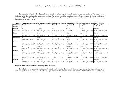
Arab Journal of Nuclear Science and Applications, 46(1), (359-373) 2013 To construct a probability plot, the sample order statistic xi or ln xi is plotted (usually on the vertical axis) against g( F ˆ ) (usually on the i horizontal axis). The mathematical expressions obtained for various probability distributions at different formulas of plotting position are presented in Table 4. The mathematical expressions represent the expected extreme wind speed in the east Cairo. The equations are obtained from 48 constructing probability plots. Table (4): mathematical expressions (predicted values) for various probability distributions at different formulas of probability position Probability Position Gumbel Weibull Normal Log-Normal Logistic Log-Logistic Hosking and Wallis xp = 9.5674g( F ˆ )+65.224 i Ln(xp)= 0.1532g( F ˆ )+4.3277 i xp = 12.909 g( F ˆ )+70.69 i Ln(xp)= 0.1876g( F ˆ )+ 4.2407 i xp = 7.169 g( F ˆ )+70.648 i Ln(xp)= 0.1042 g( F ˆ )+ 4.2401 i Hazen xp = Ln(xp) = xp = Ln(xp)= xp = Ln(xp )= F )+65.304 F )+4.3299 F )+70.96 F )+4.2446 F )+70.96 F )+4.2446 Gringorten Cunnane Blom Filliben 9.9286g( ˆ i xp = 10.074 ( ˆ F i )+65.261 xp = 10.166g( F ˆ )+65.235 i xp = Benard xp = Weibull 10.221g( ˆ i xp = F )+65.219 10.344g( ˆ F i )+65.185 10.38g( F ˆ )+65.174 i xp = 10.939g( ˆ F i )+65.021 0.1496g( ˆ i Ln( xp)= 0.1517g( ˆ F i )+4.3305 Ln( xp)= 0.153g( F ˆ )+ 4.3308 i Ln( xp)= F )+4.3311 0.1538g( ˆ i Ln( xp)= 0.1556g( ˆ F i )+4.3315 Ln(xp)= 0.1561g( ˆ i F )+4.3317 Ln( xp)= F )+4.3338 0.1641g( ˆ i 12.953 g( ˆ i xp = 13.082 g( ˆ F i )+70.96 xp = 13.165 g( F ˆ )+70.96 i xp = 13.215 g( ˆ i xp = F )+7 0.96 13.327 g( ˆ F i )+70.96 xp = 13.36 g( F ˆ )+70.96 i xp = Selection of Probability Distributions and plotting Positions 13.887 g( ˆ F i )+70.96 366 0.1887g ( ˆ i Ln(xp)= 0.1906g ( ˆ F i )+4.2446 Ln(xp)= 0.1918g( ˆ i F )+ 4.2446 Ln( xp)= F )+ 4.2446 0.1925g( ˆ i Ln(xp)= 0.1941g ( ˆ F i )+4.2446 Ln(xp)= 0.1946g ( F ˆ )+ 4.2446 i Ln(xp)= 0.2022g ( ˆ i F )+ 4.2446 7.2155 g( ˆ i xp = 7.3185 g( ˆ F i )+70.96 xp = 7.3836 g( F ˆ )+70.96 i xp = 7.423 g( ˆ i xp = F )+70.962 7.5103g( ˆ F i )+70.96 xp = 7.5361 g( F ˆ )+70.96 i xp = 7.934 g( ˆ F i )+70.962 0.1052 g( ˆ i Ln(xp)= 0.1067 g( ˆ F i )+ 4.2446 Ln(xp)= 0.1077 g( F ˆ )+ 4.2446 i Ln(xp)= 0.1082 g( ˆ i Ln(xp)= F )+4.2446 0.1095 g( ˆ F i )+ 4.2446 Ln(xp)= 0.1099 g( F ˆ )+ 4.2446 i Ln(xp)= 0.1156 g( ˆ i F )+ 4.2446 The selection of an appropriate plotting plot formula for each statistical distribution is the most important step that is generally chosen by using the goodness of fit tests. The PPCC test is a goodness-of-fit test which measures and evaluates the linearity of the probability plot.
Arab Journal of Nuclear Science and Applications, 46(1), (359-373) 2013 Comparison between eight formulas of plotting position for six probability distributions is done to choose the best plotting position and the appropriate probability distribution. The comparison is based on four test criteria namely: probability plot correlation coefficient (PPCC), root mean square error (RMSE), relative root mean square error (RRMSE) and maximum absolute error (MAE). Table 5 shows the PPCC, RMSE, RRMSE and MAE between observed and expected values for all compared distributions using different formula of plotting positions. The best distribution and plotting position is determined according to the highest PPCC and the lowest RRMSE and MAE between observed and expected values. It is found that the Normal distribution has the maximum value of PPCC and the minimum values of RMSE, RRMSE and MAE of MAWS under each plotting position when it is compared with other distributions. Moreover, The Weibull plotting position has the highest value of PPCC and the lowest values of RMSE, RRMSE and MAE under each probability distribution when it is compared with other plotting positions. The results show that the Weibull' plotting position at each distribution has slightly, highest value of PPCC and lowest value RMSE, RRMSE and MAE comparing with Benard and Filliben plotting position at the same distribution. Then, The Weibull plotting is considered the best formula for selection an appropriate distribution, followed by Benard and Filliben, respectively. However, the Hosking and Wallis plotting position at Weibull distribution is occupy third rank after Benard plotting position. The appropriate probability distribution which representing and excpecing the (MAWS) in east Cairo is Normal distribution followed by Weibull and Logistic distribution, respectively. The results of Table 5 indicate that the Weibull plotting position combined with Normal distribution give the highest fit, most reliable and accurate predictions of the MAWS east Cairo. Table (5): The test criteria of different formulas of plotting position for the six compared distributions Gumbel PPCC RMSE RRMSE MAE Weibull Weibull 0.962428 3.60902 0.054804 9.135469 Benard 0.957892 3.816265 0.057238 10.81708 Filliben 0.957542 3.831737 0.057423 10.93825 Blom 0.956298 3.886239 0.058073 11.35156 Cunnane 0.955706 3.911886 0.05838 11.54552 Gringorten 0.954684 3.955737 0.058909 11.86722 Hazen 0.952946 4.029084 0.059803 12.39603 Hosking and Wallis 0.944557 4.364136 0.065102 14.17574 Weibull 0.984423 2.317373 0.03461 5.293756 Benard 0.982095 2.424945 0.036981 5.517268 Filliben 0.981898 2.433873 0.037166 5.527232 Blom 0.981181 2.466554 0.037854 5.586213 Cunnane 0.980831 2.482686 0.038175 5.604537 Gringorten 0.980214 2.50961 0.038741 5.647132 Hazen 0.979134 2.557409 0.039703 5.709897 Hosking and Wallis 0.982013 2.414627 0.037034 5.498528 367
Page 1 and 2: Arab Journal of Nuclear Science and
Page 7: Arab Journal of Nuclear Science and
Page 13 and 14: Quantile Quantile 120 100 80 60 40
Page 15: Arab Journal of Nuclear Science and

Download - Arab Journal of Nuclear Sciences and Applications

You also want an ePaper? Increase the reach of your titles

Delete template?

Save as template?