Ray tracing - ESRF
Ray tracing - ESRF
Ray tracing - ESRF

Create successful ePaper yourself
Turn your PDF publications into a flip-book with our unique Google optimized e-Paper software.
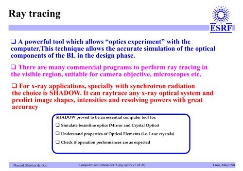
<strong>Ray</strong> <strong>tracing</strong><br />
❑ A powerful tool which allows “optics experiment” with the<br />
computer.This technique allows the accurate simulation of the optical<br />
components of the BL in the design phase.<br />
❑ There are many commercial programs to perform ray <strong>tracing</strong> in<br />
the visible region, suitable for camera objective, microscopes etc.<br />
❑ For x-ray applications, specially with synchrotron radiation<br />
the choice is SHADOW. It can raytrace any x-ray optical system and<br />
predict image shapes, intensities and resolving powers with great<br />
accuracy<br />
Manuel Sánchez del Río<br />
SHADOW proved to be an essential computer tool for:<br />
❑ Simulate beamline optics (Mirror and Crystal Optics)<br />
❑ Understand properties of Optical Elements (i.e. Laue crystals)<br />
❑ Check if operation performances are as expected<br />
Computer simulations for X-ray optics (5 of 20)<br />
Luso, May1998
<strong>Ray</strong> <strong>tracing</strong> in Optics can be easily done with computers.<br />
source<br />
Manuel Sánchez del Río<br />
image<br />
mirror<br />
Two aspects:<br />
Computer simulations for X-ray optics (6 of 20)<br />
❑ <strong>Ray</strong>s emerging from the source<br />
[source generation]<br />
❑ <strong>Ray</strong>s through Optical Elements<br />
[Geometrical and Physical models]<br />
Luso, May1998
What CAN be calculated with SHADOW?<br />
❑ Beam Cross sections (focal spot, etc). Effects of:<br />
❑ Energy resolution<br />
Manuel Sánchez del Río<br />
❑ source characteristics (dimensions, depth, emittances...)<br />
❑ vignetting (finite optical elements, slits, etc.)<br />
❑ aberrations<br />
❑ thermal deformations<br />
❑ waviness and roughness errors of mirrors<br />
❑ Flux & Power (number of photons at sample, absorbed/transmitted power, etc.)<br />
❑ Other parameters (i.e polarization transfer)<br />
Computer simulations for X-ray optics (11 of 33)<br />
PSI, Feb 1998
What CANNOT be calculated with SHADOW?<br />
(Ideas for future developments...)<br />
1) Physical models:<br />
❑ Sources: ➟X-ray tubes. ➟Elliptical undulators. ➟Tapered undulators. ➟General wigglers.<br />
➟Wiggler exact calculation.<br />
❑ Optics: ➟Extended energy range (E> 100 keV). ➟Compton absorption cross section.<br />
➟Coherence (holography, phase contrast, speckle patterns...).<br />
❑ Gratings: ➟Efficiency model.<br />
❑ Crystals: ➟Any crystal. ➟External Rocking Curve. ➟Transmitted beam (phase shifters,<br />
diamond monochromators). ➟Improved mosaic model (transition Perfect -><br />
Mosaic). ➟Bent crystal reflectivity. ➟Beam penetration in the crystal.<br />
❑ New devices: ➟Bragg Fresnel Lenses. ➟CRL. ➟Non-sequential systems (i.e. Multiple<br />
mirror arrays).<br />
2) Program structure:<br />
➟Migration Fortran -> C ?. ➟Dynamic arrays (any number of rays). ➟Test set. ➟➟User<br />
program macros. ➟Global optimization. ➟Improve user-friendly interface<br />
Manuel Sánchez del Río<br />
Computer simulations for X-ray optics (12 of 33)<br />
PSI, Feb 1998
1- Simplest case: The spherical source.<br />
Source Models in SHADOW<br />
❑ 1st Solution. Grid Generation of <strong>Ray</strong>s:<br />
x = (0,0,0)<br />
v = (0, cos 2π(i/N), sin 2π(i/N) )<br />
i=0,...N<br />
❑ 2nd Solution. Random Generation of <strong>Ray</strong>s:<br />
x = (0,0,0)<br />
v = (0, cos (2πnr), sin (2πnr) )<br />
n r = random number in [0,1] with flat probability<br />
distribution function given by the computer random<br />
generator.<br />
Manuel Sánchez del Río -9-<br />
Experiments Division<br />
Programming Group<br />
Grenoble, January 18, 1994<br />
EUROPEAN SYNCHROTRON RADIATION FACILITY
2- General case: The Gaussian [or any kind of distribution f ] generator.<br />
❑ 1st Solution. Deterministic generator:<br />
❑ 2nd Solution. Stochastic generator:<br />
x = (0,0,0)<br />
v = (0, cos θi , sin θi) I = f (θi )<br />
θi = θmin + (i/N) (θmax - θmin) i = 0, ..., N<br />
x = (0,0,0)<br />
v = (0, cos θ i , sin θ i)<br />
θ i are numbers generated randomly but following<br />
the gaussian [or f] distribution.<br />
How to get them?<br />
Manuel Sánchez del Río -10-<br />
Experiments Division<br />
Programming Group<br />
Grenoble, January 18, 1994<br />
EUROPEAN SYNCHROTRON RADIATION FACILITY
The inversion method<br />
f(φ)<br />
cdf(φ)<br />
φ<br />
φ<br />
1<br />
0<br />
❑ Given the probability distribution, i.e.<br />
f ( φ)<br />
=<br />
1<br />
------------- exp i<br />
κ 2π<br />
φ2<br />
2κ2 ⎛– -------- ⎞<br />
⎝ ⎠<br />
❑ Calculate the Cumulative Distribution Function (cdf)<br />
cdf ( φ)<br />
= f ( φ)dφ<br />
Manuel Sánchez del Río -11-<br />
Experiments Division<br />
Programming Group<br />
Grenoble, January 18, 1994<br />
φ<br />
∫<br />
0<br />
❑ Calculate the inverse function<br />
Φ( n)<br />
cd f 1 – = ( n)<br />
If now n samples an interval [0,1] with flat<br />
probability distribution, Φ(n) samples an interval<br />
(-∞, +∞) with probability distribution f.<br />
❑ If n ∈[n1 ,n2 ] then the φ interval is [φ1 ,φ2 ] with<br />
n1=cdf(φ1) and n2=cdf(φ2) EUROPEAN SYNCHROTRON RADIATION FACILITY
The synchrotron sources<br />
e -<br />
ϑ<br />
Ψ<br />
Manuel Sánchez del Río<br />
Dipoles Wigglers Undulators<br />
hϖ<br />
Source Size 0.45mm(H)x0.30mm(V)<br />
Source Divergences<br />
hϖ<br />
e -<br />
Bending Magnet and Wiggler Radiation Undulator Radiation<br />
Computer simulations for X-ray optics (8 of 20)<br />
hϖ<br />
Undulator Divergences<br />
Luso, May1998
Tracing an Optical Element (i.e. MIRRORS)<br />
1) Geometrical Model<br />
source = { ray i , i=1...N }<br />
trajectory: x = x start + t v<br />
Surface equation<br />
Manuel Sánchez del Río<br />
f(x,y,z) = 0<br />
=> Intercept point<br />
source<br />
ray = ( x, ...) v,<br />
Computer simulations for X-ray optics (9 of 20)<br />
n = grad(f)<br />
Optical Element<br />
<strong>Ray</strong> <strong>tracing</strong> equation. Here (Mirrors) the specular reflectivity is applied:<br />
θin = θout ; vin , n and vout coplanar. In vectorial notation: vout = vin - 2 vin 2) Physical Model<br />
Reflectivity ~ probability of observation or intensity after reflection.<br />
We must include a new variable in the ray: Iout = Iin R(E,θ,...)<br />
In fact, R is polarization-dependent, so it is better to store the<br />
I = | Es exp(iφs ) + Ep exp(iφp ) | 2<br />
Electric field:<br />
ray i = ( x, v, i, flag, E s , E p , φ s , φ p , φ g , 2π/λ)<br />
v in<br />
v out<br />
image<br />
Luso, May1998
Focus is not perfect because of :<br />
❑ aberrations<br />
❑ source dimensions and depth [emittances]<br />
❑ waviness and roughness errors of mirrors<br />
All these effects can be studied by ray-<strong>tracing</strong>. Example:<br />
circular source (diameter: 10 μm)<br />
divergences: 100 μrad<br />
p=30m<br />
θ=89.8 deg<br />
q=10m<br />
Toroidal Mirror<br />
Ellipsoidal Mirror<br />
Manuel Sánchez del Río -13-<br />
Experiments Division<br />
Programming Group<br />
Ferrara, March 11 1994<br />
EUROPEAN SYNCHROTRON RADIATION FACILITY
The model is not sufficient: The ray may not exist after the mirror [it is absorbed]<br />
We must extend the model<br />
E s out = E s in * R s<br />
E p out = E p in * R p<br />
θ inc=89.9deg<br />
Reflectivity ~ probability of observation<br />
or intensity after reflection.<br />
We must include a new variable in the ray: I<br />
I out = I in R(E,θ,...)<br />
In fact, R is polarization-dependent, so it is<br />
better to store the Electric field:<br />
I = | E s exp(iφ s ) + E p exp(iφ p ) | 2<br />
ray i = ( x, v, i, flag, E s , E p , φ s , φ p , φ g , 2π/λ)<br />
This permits also to work with polarized light, analyze the polarization degree<br />
and polarization properties through the beamline.<br />
|Es|=|Ep| φp = φs + π/2<br />
circular pol. light<br />
Rs, Rp and phase change are given by a physical model of reflectivity. For mirrors<br />
the Fresnel equations are coded in the program.<br />
Manuel Sánchez del Río -14-<br />
Experiments Division<br />
Programming Group<br />
Ferrara, March 11 1994<br />
EUROPEAN SYNCHROTRON RADIATION FACILITY
Other O.E.s can be easily modeled:<br />
❑ Multilayers:Mirror + “New” Reflectivity curve.<br />
Geometry: Reflectivity:<br />
θ graz = 0.42 deg<br />
n pairs (100)<br />
Substrate (Si)<br />
❑ CRYSTALS: Symmetric Bragg Case =Mirror + “New” Reflectivity curve given by the DTD.<br />
Geometry: Reflectivity:<br />
v in<br />
θ<br />
v out<br />
v out = v in - 2 v in⊥<br />
Light element Si (41.4 A)<br />
Heavy element W(10.3 A)<br />
Manuel Sánchez del Río -15-<br />
Experiments Division<br />
Programming Group<br />
Ferrara, March 11 1994<br />
EUROPEAN SYNCHROTRON RADIATION FACILITY
Other O.E.s can be easily modeled:<br />
❑ LENSES: interface between two mediaof refractive indeces n 1 and n 2<br />
n 1<br />
n 2<br />
k in k out<br />
❑ CRYSTALS: Symmetric Bragg Case = Mirror + “New” Reflectivity curve given by the DTD.<br />
θ<br />
u n<br />
n 1(k in x u n) = n 2(k out x u n)<br />
Geometry: Reflectivity:<br />
v in<br />
v out<br />
v out = v in - 2 v in<br />
[Hetch, Optics]<br />
Manuel Sánchez del Río -7-<br />
Experiments Division<br />
Programming Group<br />
Grenoble, January 18, 1994<br />
EUROPEAN SYNCHROTRON RADIATION FACILITY
mλ = d (sin θ in + sin θ out )<br />
or<br />
k out = k in + G ||<br />
Gratings: Geometrical Model<br />
k in<br />
G || =m (2π/d) u ||<br />
Manuel Sánchez del Río -11-<br />
Computer simulations for X-ray optics (<strong>Ray</strong>-<strong>tracing</strong> and More)<br />
LSBarcelona, 13 Dec 1996<br />
θ in<br />
[k 1 ,k 3 ] k 1<br />
k 3<br />
k 2<br />
slit<br />
θ out k out<br />
m=2<br />
m=1<br />
m=0<br />
m=-1<br />
m=-2<br />
EUROPEAN SYNCHROTRON RADIATION FACILITY
Gratings: Monochromators<br />
❑ They combine the dispersive effect of the grating + focusing effect of curvature<br />
❑ Can be analyzed by ray-<strong>tracing</strong><br />
❑ Focusing equations: Generalized case of mirror’s focusing equations<br />
Efficiency [%]<br />
0.4 -<br />
0.0 -<br />
1 1<br />
-- + --<br />
p q<br />
cosθ1 + cosθ2<br />
-----------------------------------<br />
Rs Manuel Sánchez del Río -12-<br />
Computer simulations for X-ray optics (<strong>Ray</strong>-<strong>tracing</strong> and More)<br />
LSBarcelona, 13 Dec 1996<br />
=<br />
( cosθ1<br />
) 2<br />
( cosθ2<br />
)<br />
-------------------p<br />
2<br />
+ --------------------q<br />
0 100<br />
Energy [eV]<br />
200<br />
=<br />
cosθ1 + cosθ2<br />
-----------------------------------<br />
Rt (Not considered in SHADOW)<br />
EUROPEAN SYNCHROTRON RADIATION FACILITY
Mirror optics<br />
Surface errors and their implementation in SHADOW<br />
❑ Figure: (macroscopic ondulations of the surface, giving the surface shape (plane, spherical...),<br />
and deformations produced by the manufacturing errors, thermal loads and mechanical<br />
stress.<br />
In SHADOW we use a mapping of the surface (from FEM, etc.) or include directly the error<br />
parameters (surface radius,...)<br />
❑ Slope errors: generally considered as sinusoidal-like variations of the surface shape. It<br />
spreads the image in the focal plane due to the deflection of the incident rays at different<br />
angles.<br />
In RT <strong>tracing</strong> we use a reflection model with a mapping of the surface (d~mm>>λ, ie., geometrical<br />
optics regime)<br />
❑ Roughness: Random irregularities in the micro or sub-microscopic scale, which depends<br />
on the manufacture processes and materials. It increases the scattering of the photon beam,<br />
producing a blur of the image in the focal point.<br />
In RT, as it is impossible to characterize deterministically the surface, a statistical approach<br />
based on the diffraction theory is used.<br />
Manuel Sánchez del Río<br />
Computer simulations for X-ray optics (13 of 33)<br />
PSI, Feb 1998
Mirror optics: Thermal Analysis (figure error)<br />
Manuel Sánchez del Río<br />
Power density on first crystal<br />
Spot without thermal load<br />
Crystal deformation<br />
Spot with thermal load<br />
Computer simulations for X-ray optics (14 of 33)<br />
BL 2 SHADOW/<br />
ANSYS calculation.<br />
Source:<br />
Wiggler<br />
λu = 125 mm<br />
N = 12<br />
E = 6.04 GeV<br />
σx = 69 μm<br />
σz = 47 μm<br />
εx = 610 -7 rad.cm<br />
εz = 610 -8 rad cm<br />
Optics:<br />
C,Be,Al attenuators<br />
Flat Mirror<br />
Double-xtal monochromator<br />
First crystal: cryogenically<br />
cooled<br />
θ B = 3.78 degrees<br />
(sagittally focusing<br />
M=1/3)<br />
Cylindrical mirror<br />
(M=1/4.3)<br />
Power on first crystal:<br />
2.6 kW<br />
PSI, Feb 1998
Mirror optics: waviness (slope error) analysis<br />
Focal spot simultions for BL1<br />
(Microfocus):<br />
Source<br />
Undulator placed in a low beta<br />
section<br />
λu = 46mm<br />
N = 33<br />
E = 6.04 GeV<br />
σx = 59 μm<br />
σz = 11 μm<br />
εx = 4 10 -7 rad.cm<br />
εz = 4 10-9 rad cm<br />
III harmonic @ 7144 eV<br />
Ellipsoidal mirror M=1/10<br />
Slope error 0.8”<br />
Manuel Sánchez del Río<br />
Slope<br />
error:<br />
Sinusoidal<br />
Toroidal Mirror Ellipsoidal Mirror<br />
Ellipsoidal Mirror + 0.8” slope error<br />
Computer simulations for X-ray optics (15 of 33)<br />
C. Riekel et al.<br />
Rev Sci Instrum 63<br />
974-981 (1992)<br />
Multi- frequency<br />
M. Sanchez del Rio et al.<br />
Nucl. Ins. Meth. A319<br />
170-177 (1992)<br />
PSI, Feb 1998
Mirror optics:<br />
Slope/Figure errors with real profiles I<br />
R. Signorato & M. Sanchez del Rio, SPIE Proceedings 3152 (1997)<br />
(ID12a)<br />
Manuel Sánchez del Río<br />
F1<br />
7.64 m<br />
Computer simulations for X-ray optics (16 of 33)<br />
.3 m<br />
M=0.2<br />
42.77 m<br />
❑ R1 = 4809 m (concave)<br />
❑ R2 = 154232 m (convex)<br />
❑ Expected focal position ~ 17m<br />
❑ Theoretical focal FWHM = 37 x 0.2 ~ 8 μm<br />
❑ Incuding Slope Error = 5μrad x 8m x 2 mirrors = 80 μm<br />
Results:<br />
❑ 22 μm FWHM<br />
❑ Satellite structures<br />
❑ Best focus fount at 7.64 m from M2<br />
source<br />
37 μm<br />
PSI, Feb 1998
Slope/Figure errors with real profiles II<br />
Mirror metrology<br />
❑ Slopes measured at the <strong>ESRF</strong> LTP<br />
❑ Standard data reduction (linear detrending, slope error rms, PSD) done with XOP.<br />
❑ Profiles used to create a surface mapping (transversal replication) to be included in<br />
SHADOW (by its PRESURFACE tool).<br />
Manuel Sánchez del Río<br />
Computer simulations for X-ray optics (17 of 33)<br />
PSI, Feb 1998
Slope/Figure errors with real profiles III<br />
<strong>Ray</strong>-<strong>tracing</strong>/Experiment comparison<br />
Manuel Sánchez del Río<br />
Computer simulations for X-ray optics (18 of 33)<br />
A = experimental<br />
B = calculated<br />
PSI, Feb 1998
Slope/Figure errors with real profiles IV<br />
Focal images at positions E (@7.62m from M2) and T (@17.14 m from M2)<br />
Manuel Sánchez del Río<br />
Computer simulations for X-ray optics (19 of 33)<br />
PSI, Feb 1998
Imaging properties of spherically bent crystals<br />
Backlighting scheme<br />
Mesh grid<br />
X-ray source<br />
Manuel Sánchez del Río<br />
Image of source<br />
Film (image of mesh)<br />
<strong>Ray</strong> <strong>tracing</strong> of curved crystal optics (16 of 30)<br />
Rowland circle geometry<br />
2R R=R~>100-180 mm<br />
θ B ~ 80-88 deg<br />
λ = 6.63 A<br />
Resolution better than 10 µm<br />
Ref: M. Sanchez del Rio, A. Ya Faenov,<br />
V. M. Dyakin, T. A. Pikuz, S. A. Pikuz,<br />
V. M. Romanova and T. A. Shelkovenko,<br />
Physica Scripta 55, 735-740 (1997)<br />
Weimar, Oct 4, 1999
Imaging properties of spherically bent crystals<br />
<strong>Ray</strong> <strong>tracing</strong> simulation<br />
Manuel Sánchez del Río<br />
θ B [deg] c [cm] R [cm] a [cm] b [cm]<br />
Conf A 86 9.98 10.00 6.25 25.00<br />
Conf B 86 18.56 18.60 11.63 46.5<br />
Conf C 80 9.85 10.00 6.25 25.0<br />
<strong>Ray</strong> <strong>tracing</strong> of curved crystal optics (17 of 30)<br />
A central<br />
A lateral<br />
B central<br />
point<br />
source<br />
10 µm 100 µm<br />
2 2.1 2.1 2.9<br />
5 5.5 9.4 ~25<br />
3 3 4.2 ~18<br />
B lateral 4 4.3 7.7 ~25<br />
C central<br />
3.3 3.3 3.3 4<br />
Weimar, Oct 4, 1999<br />
1000<br />
µm<br />
C lateral 10 11 18 No resolution
Collimation of X-rays (from plasmas)<br />
<strong>Ray</strong> <strong>tracing</strong> simulation of spherically bent crystals<br />
We studied the effects of<br />
1) Surface shape and geometrical errors<br />
2) Crystal size (entrance pupil)<br />
3) Source depth abd width<br />
4) Incident angle<br />
Manuel Sánchez del Río<br />
Ref: M. Sanchez del Rio, M. Fraenkel, A.<br />
Ziegler, A. Ya. Faenov and T. A. Pikuz,<br />
Rev. Sci. Instrum. 70(3), 1614-1620, 1999<br />
<strong>Ray</strong> <strong>tracing</strong> of curved crystal optics (18 of 30)<br />
0.6<br />
0.4<br />
0.2<br />
0.0<br />
-0.2<br />
-0.4<br />
80<br />
60<br />
40<br />
20<br />
0<br />
-0.6 -0.4 -0.2 0.0 0.2 0.4 0.6<br />
-0.6<br />
-0.6 -0.4 -0.2 0.0 0.2 0.4 0.6<br />
0.6<br />
0.4<br />
0.2<br />
0.0<br />
-0.2<br />
-0.4<br />
140<br />
120<br />
100<br />
50 µm source<br />
200 µm source<br />
-0.6<br />
-0.6 -0.4 -0.2 0.0 0.2 0.4 0.6<br />
Weimar, Oct 4, 1999
Introduction V:<br />
Perfect crystals in asymmetric diffraction<br />
In Reflection (Bragg) mode<br />
S1<br />
Δθ 1<br />
Manuel Sánchez del Río<br />
Δθ 2<br />
S 2<br />
<strong>Ray</strong> <strong>tracing</strong> simulations for crystal optics (7 of 23)<br />
In Transmission (Laue) mode<br />
M. Sanchez del Rio & F. Cerrina M. Sanchez del Rio et al.<br />
Rev. Sci. Instrum 63 (1) 936 (1992) Nucl. Ins. Meth. A347 338 (1994)]<br />
S 1<br />
k 1<br />
d<br />
θ B<br />
k 2<br />
S 2<br />
SPIE, July 22, 1998
Theory I<br />
Geometrical model<br />
S 1<br />
k' 1<br />
k1<br />
Manuel Sánchez del Río<br />
θ 1<br />
k 1<br />
d<br />
θ B<br />
B H<br />
B H<br />
k' 2<br />
1<br />
= ⎛– -- ⎞uB ⎝ d⎠<br />
α>0<br />
θ 2<br />
k 2<br />
k2<br />
S 2<br />
<strong>Ray</strong> <strong>tracing</strong> simulations for crystal optics (8 of 23)<br />
❑ Elastic scattering: k2 = k1 ❑Boundary conditions: k2 = k1 + BH ⇔<br />
– sinθ2<br />
= sinθ1<br />
Gratings<br />
λ<br />
– -- sinα<br />
d<br />
mλ = d’ (sin θ in + sin θ out )<br />
or<br />
k out = k in + G ||<br />
d/sinα = d’ /m<br />
Tracing condition (Grating eq.)<br />
k in<br />
G || =m (2π/d’) u ||<br />
θ in<br />
θ out k out<br />
m=-2<br />
m=-1<br />
m=0<br />
m=1<br />
m=2<br />
SPIE, July 22, 1998
Theory II<br />
Physical model: Dynamical Theory of Diffraction<br />
C 1<br />
C 2<br />
=<br />
=<br />
e iϕ – 1t o<br />
e iϕ – 2t o<br />
Manuel Sánchez del Río<br />
z<br />
=<br />
❑ BRAGG case<br />
(Zachariasen 1945)<br />
(Compact, general (thin/thick, Laue/Bragg), with absorption, general expression for τ, F H )<br />
valid for perfect flat crystals<br />
R( θ)<br />
❑ LAUE case R( θ)<br />
ϕ1 2π koδ'o = ----------γ<br />
o<br />
ϕ2 2π koδ''o = ------------γ<br />
o<br />
1 – b b<br />
-----------Ψ<br />
2 o – --τ<br />
2<br />
q = bΨHΨ H<br />
γ o<br />
b ≈ -----γ<br />
H<br />
where<br />
δ'<br />
⎛ o⎞<br />
=<br />
⎝δ''o⎠ τ<br />
1<br />
--<br />
b<br />
IH = ----- =<br />
Io 1<br />
--<br />
b<br />
IH = ----- =<br />
Io <strong>Ray</strong> <strong>tracing</strong> simulations for crystal optics (9 of 23)<br />
1<br />
--<br />
b<br />
x1x2 c ( 1 – c2) --------------------------------c2x2<br />
– c1x1 1<br />
--<br />
b<br />
x1x2 c ( 1 – c2) --------------------------------x2<br />
– x1 1<br />
-- ψ<br />
2 o z q z 2<br />
⎛ – ⎛ ± + ⎞⎞<br />
⎝ ⎝ ⎠⎠<br />
2<br />
2<br />
x<br />
⎛ 1⎞<br />
=<br />
⎝x2⎠ 1<br />
---- B<br />
2<br />
ko 2 H 2 ke = ( + ( o ⋅ BH ) ) τ ≈ 2( θ– θB) sin2θ<br />
Ψ H<br />
=<br />
z q z 2<br />
– ⎛ ± + ⎞<br />
⎝ ⎠<br />
----------------------------------ψ<br />
H<br />
e2 mc2 --------- 1<br />
---<br />
V<br />
λ2<br />
----- ( f<br />
π<br />
o + f ' + f '')<br />
e<br />
n 2πi H r ⎛ ( ⋅ n)<br />
⎞<br />
∑<br />
K<br />
⎝ ⎠<br />
n ∈ unitcell<br />
SPIE, July 22, 1998
Perfect crystals IV<br />
Tracing a polychromatic divergent bem on a flat symmetrical xtal<br />
Manuel Sánchez del Río<br />
point source: image plane<br />
1: 3 Ι Energy lines<br />
2: continous spectrum<br />
θ Β<br />
Computer simulations for X-ray optics (23 of 33)<br />
PSI, Feb 1998
Benchmarks I<br />
Phase space<br />
Study the changes induced by a Si 111 crystal in the (z,z’) space, E= 8 keV, α = 5 deg<br />
z<br />
z z'<br />
z'<br />
Manuel Sánchez del Río<br />
Dependency in energy<br />
<strong>Ray</strong> <strong>tracing</strong> simulations for crystal optics (10 of 23)<br />
SPIE, July 22, 1998
Benchmarks II<br />
Du Mond diagrams (J.W.M. Du Mond, Phys. Rev. 52 (1937) 872)<br />
(+,+) Si 111, 12 keV<br />
Manuel Sánchez del Río<br />
<strong>Ray</strong> <strong>tracing</strong> simulations for crystal optics (11 of 23)<br />
SPIE, July 22, 1998
Benchmarks III<br />
Few equations<br />
Focusing equations for a monochromatic beam (like for gratings):<br />
1<br />
p<br />
Manuel Sánchez del Río<br />
+ 1<br />
q = sin 1 + j sin 2j<br />
Rs<br />
For Bragg symmetrical crystals ( 1 = 2 = 0):<br />
Spectral resolution:<br />
0<br />
= E<br />
E0<br />
= cot 0<br />
1 1<br />
+<br />
p q = 2 sin 0<br />
;<br />
Rs<br />
;<br />
sin 2 1<br />
p + sin2 2<br />
q<br />
1<br />
p<br />
+ 1<br />
q =<br />
= sin 1 + j sin 2j<br />
Rt<br />
<strong>Ray</strong> <strong>tracing</strong> simulations for crystal optics (12 of 23)<br />
2<br />
Rt sin 0<br />
q<br />
! 2 D +( geom + ss) 2 s<br />
cot 0 = ! 2 D +<br />
p<br />
R sin 1<br />
, 1 src + s1<br />
p<br />
2<br />
(1)<br />
(2)<br />
cot 0<br />
(3)<br />
SPIE, July 22, 1998
High resolution I<br />
Collimating pre-mirror (Δ src ~ 0)<br />
Mirror (3 mrad) and (+,-) Si111. E=10 keV, source 85 μm 185 μrad<br />
Manuel Sánchez del Río<br />
Mirror E[eV ] I [ rad]<br />
No mirror 8.47 0.99 1008 38 158 24<br />
Parabolic 1.27 0.05 1004 20 3.9 0.3<br />
Elliptical 1.27 0.05 1004 20 3.9 0.3<br />
Cylindrical 1.28 0.06 1002 18 4.4 0.3<br />
Cylindrical+1" slope 1.44 0.15 1000 20 20.7 2.9<br />
Cylindrical+2" slope 2.33 0.12 1008 18 38.5 3.6<br />
<strong>Ray</strong> <strong>tracing</strong> simulations for crystal optics (13 of 23)<br />
SPIE, July 22, 1998
High resolution II<br />
Rowland bending (p/(R sin θ B )= 1)<br />
Manuel Sánchez del Río<br />
θ B +δ<br />
θ B<br />
θ B −δ<br />
(+,-) Si111, 10 keV, source 85 μm 185 μrad<br />
System I1 I2 E1[eV ] E2[eV ]<br />
at- at 413 14 307 12 8.92 0.55 8.71 0.69<br />
Rowland(1:1)- at 414 25 65 9 1.44 0.06 1.23 0.24<br />
Rowland(concave)-Rowland(convex) 399 12 296 10 1.44 0.07 1.32 0.06<br />
Out-Rowland(1:3)- at 408 18 36 3 8.2 0.9 2.1 0.5<br />
<strong>Ray</strong> <strong>tracing</strong> simulations for crystal optics (14 of 23)<br />
θ B<br />
θ B<br />
SPIE, July 22, 1998
High resolution III<br />
Normal incidence (Masciovecchio et al, NIM B111 (1996) 181)<br />
Manuel Sánchez del Río<br />
ΔE=0.28 meV (e -M =0.13)<br />
ΔE=0.45 meV (e -M =0.2)<br />
ΔE=0.5 meV [experimental]<br />
Si 13,13,13, ~ 25 keV, θ B =89.98 deg, R=250 cm<br />
<strong>Ray</strong> <strong>tracing</strong> simulations for crystal optics (15 of 23)<br />
SPIE, July 22, 1998
High resolution IV<br />
Multicrystal dispersive system<br />
Manuel Sánchez del Río<br />
E=14413 eV<br />
Si 10,6,4 α=20 deg<br />
<strong>Ray</strong> <strong>tracing</strong> simulations for crystal optics (16 of 23)<br />
Si 4,2,2 α=0<br />
Si 10,6,4 α=-20 deg<br />
ΔE=6.3 meV (6.7 from refs)<br />
Si 9,7,5 α=75.4 deg<br />
Si 9,7,5 α=-75.4 deg<br />
ΔE=1.65 meV (1.57 theoretically from ref)<br />
Nested monochromator<br />
Isikawa et al. RSI 63 (1992) 1015<br />
Chumakov et al. SPIE 3151(1997) 262<br />
Alp et al. APS Res. 1(1998) 9<br />
Highly asymmetric<br />
monochromator<br />
Chumakov et al. NIM A383(1996) 642<br />
SPIE, July 22, 1998
Focusing optics I<br />
Polychromatic focusing with plane Laue crystals I<br />
Manuel Sánchez del Río<br />
s 1<br />
λ,θ Β<br />
λ’,θ’ Β<br />
λ”,θ” Β<br />
Pseudo-focusing effect of a Laue crystal for a white incident divergent beam. The selective<br />
reflections on the Bragg planes convert the divergent beam into a convergent one.<br />
❑ magnification factor M<br />
s<br />
2<br />
Δθ<br />
1<br />
= ---- = --------- =<br />
s<br />
1<br />
Δθ<br />
2<br />
❑ best focus expected at a distance of s2 = Ms1 1<br />
--<br />
b<br />
❑ Symmetrical Laue: M=1 ( i.e. a 1:1 focussing device)<br />
❑ Asymmetrical Laue: M=1/b => M(E) => Dispersive System=> Focus size is a function of ΔE<br />
<strong>Ray</strong> <strong>tracing</strong> simulations for crystal optics (17 of 23)<br />
s 2<br />
SPIE, July 22, 1998
Focusing optics I<br />
Polychromatic focusing with plane Laue crystals II<br />
Manuel Sánchez del Río<br />
Undulator Source<br />
top view<br />
28 m<br />
Layout of the experimental station at the Troika<br />
beamline.<br />
The monochromator is composed by the Laue<br />
diamond and Bragg Ge crystals in the nondispersive<br />
arrangement.<br />
Inset: Incidence angles for the x-ray beam when<br />
the diamond crystal is set to diffract photons<br />
with energy of 9100 eV<br />
slit<br />
1 m<br />
<strong>Ray</strong> <strong>tracing</strong> simulations for crystal optics (18 of 23)<br />
Ge<br />
image planes<br />
112 cm<br />
transmitted beam<br />
<br />
125.6<br />
<br />
15.6 55<br />
Diamond Crystal<br />
diffracted beam<br />
SPIE, July 22, 1998
Focusing optics I<br />
Polychromatic focusing with plane Laue crystals III<br />
Manuel Sánchez del Río<br />
<strong>Ray</strong> <strong>tracing</strong> simulations for crystal optics (19 of 23)<br />
M. Sanchez del Rio et al, Rev Sci Instrum, 66 (11)<br />
5148- 5152, Nov 1995<br />
0.4 cm<br />
0.3 cm<br />
0.2 cm<br />
0.1 cm<br />
0.05 cm<br />
0.8 cm<br />
SPIE, July 22, 1998
Focusing optics III<br />
Sagittal bending<br />
Two aspects that can be analyzed:<br />
1) The effects of surface shape:<br />
• ❑ Anticlastic effect<br />
• ❑ Alignment<br />
• ❑ Loss of cylindrical shape<br />
• ❑ Spurious errors left by ribs<br />
• ❑ Conical surface: Ice & Sparks, JOSA<br />
A11 (1994) 1265<br />
Manuel Sánchez del Río<br />
p q<br />
2) beam transmission as a function of<br />
the angular divergence [Sparks et al.,<br />
NIM 172 (1980) 237]. The<br />
M=1:3=0.33 is optimal to focus divergent<br />
beams.<br />
M=q/p=1:3<br />
<strong>Ray</strong> <strong>tracing</strong> simulations for crystal optics (20 of 23)<br />
5 mrad<br />
2.5 mrad<br />
1 mrad<br />
SPIE, July 22, 1998
Diffraction & Coherence I<br />
Fraunhofer diffraction pattern from a slit<br />
Coherent &<br />
collimated beam (8 keV)<br />
Manuel Sánchez del Río<br />
10 cm<br />
Fraunhofer Diffraction by a slit<br />
Diffraction Pattern<br />
<strong>Ray</strong> <strong>tracing</strong> simulations for crystal optics (21 of 23)<br />
25 microns<br />
5 microns<br />
12.5 microns<br />
SPIE, July 22, 1998
Diffraction & Coherence II<br />
Fraunhofer diffraction after a symmetrical/asymmetrical crystal<br />
The conservation and propagation of transversal coherence can be studied from the visibility of the diffraction patterns<br />
Example: Degradation of the transversal coherence when using asymmetric crystal (which produce chromatic aberrations)<br />
[S. Brauer et al., J. Synchr. Rad. 2 (1995) 163]<br />
Si 111, α=0, α=0.15 deg<br />
8 keV, ΔE~ 1 eV<br />
Manuel Sánchez del Río<br />
α=0<br />
8000.0eV<br />
8000.5 eV<br />
<strong>Ray</strong> <strong>tracing</strong> simulations for crystal optics (22 of 23)<br />
α=0.15 deg<br />
SPIE, July 22, 1998
Introduction<br />
They are formed by a large number of small perfect crystallites of microscopical or submicroscopical<br />
size, which are oriented almost, but not exactly parallel to each other<br />
The most extensively used is Highly Oriented Pyrolithic Graphite (HOPG), produced by<br />
Advanced Ceramics (USA), Optigraph (Russia) and Panasonic (Japan). Typical mosaicity values<br />
go from 0.1 to 0.5 deg<br />
❑ Wider reflectivity curve than perfect crystals ~ ∆E/E ~ 10 -2<br />
❑ Lower peak reflectivity but higher integrated reflectivity<br />
❑ Well established theory Bacon & Lowde Acta Crystall. 1 (1948) 303 and Zachariasen’s book<br />
(1945)<br />
❑ The theory fails when using narrow beams due to possible macrostructures of about 40 x 400<br />
microns: Freund et al. SPIE 2856 (1996) 68<br />
❑ Macrostructures have been seen by x-ray topography: Ohler et al., NIM B129 (1997) 257<br />
❑ We studied the focusing properties [SPIE vol. 3448, 246-255, 1998]. We found that the existence<br />
or not of macrostructures depend on the particular sample [SPIE vol. 3773, 1999].<br />
Manuel Sánchez del Río<br />
<strong>Ray</strong> <strong>tracing</strong> of curved crystal optics (20 of 30)<br />
Weimar, Oct 4, 1999
Focusing properties (von Hamos geometry, 1932)<br />
TOP<br />
source<br />
S<br />
SIDE<br />
ω<br />
w<br />
Manuel Sánchez del Río<br />
ww<br />
ω' = ω + 2 τ sin θ Β<br />
SS<br />
image<br />
<strong>Ray</strong> <strong>tracing</strong> of curved crystal optics (21 of 30)<br />
❑ Mosaic crystals present a defocusing effect in the<br />
plane perpendicular to the diffraction plane<br />
❑ They present a parafocusing effect in the<br />
diffraction plane:<br />
• ❑ focusing of monochromatic radiation in M=1:1<br />
• ❑ Chromatic aberrations in the diffraction plane<br />
• ❑Aberrations produced by the beam penetration in the crystal bulk<br />
Weimar, Oct 4, 1999
Mosaic Crystals:<br />
are formed by a large number of small perfect crystallites of microscopical or<br />
submicroscopical sizes, which are oriented almost, but not exactly parallel to each other.<br />
Assumptions:<br />
1-The relative displacements of the crystallites are assumed large compared with the<br />
x-ray coherence width: No relationship between the scattering from various cristallites.<br />
2- Scattering planes are defined by the direction of their normal, and the distribution of<br />
the normals of the different crystallites is in good approximation gaussian with standard<br />
deviation κ<br />
3- κ is large compared with the Darwin width or width of the diffraction profile crystallite.<br />
θ D<br />
θ D<br />
Reflection Mode:<br />
focussing 1:1 in<br />
diffraction plane.<br />
Transmission Mode<br />
Manuel Sánchez del Río -17-<br />
Experiments Division<br />
Programming Group<br />
Ferrara, March 11 1994<br />
EUROPEAN SYNCHROTRON RADIATION FACILITY
0.4 deg fwhm<br />
Bragg case<br />
Mosaic Crystals diffraction profiles<br />
0.2 deg fwhm<br />
17 keV<br />
8 keV<br />
3 keV<br />
Diffraction profile in Bragg case:<br />
Manuel Sánchez del Río -18-<br />
Experiments Division<br />
Programming Group<br />
Ferrara, March 11 1994<br />
r( Δ)<br />
a<br />
= ------------------------------------------------------------------------------<br />
1 + a + 1+ 2acoth(<br />
A 1 + 2a)<br />
Diffraction profile in Laue case:<br />
r( Δ)<br />
= sinh(<br />
Aa)<br />
exp(<br />
– A( 1 + a)<br />
)<br />
with:<br />
w( Δ)Qsp<br />
; 1<br />
a = ---------------------- =<br />
--<br />
μ μ<br />
A<br />
η sp<br />
μt<br />
= ------------sin<br />
θ B<br />
; = w( θ– θD)Qsp ;<br />
1<br />
---------- e<br />
2π<br />
Δ2 2κ 2<br />
– ⁄ ( ) ( Fx ⁄ vo) 2 λ 3<br />
---------------------------sin2θ<br />
B<br />
Q p = Qs cos2θ<br />
B<br />
EUROPEAN SYNCHROTRON RADIATION FACILITY
<strong>Ray</strong> <strong>tracing</strong> modeling with SHADOW<br />
k in , |k|=1<br />
y<br />
β<br />
θ D<br />
α<br />
φ<br />
Manuel Sánchez del Río<br />
z<br />
Ref: M. Sanchez del Rio et al. Rev. Sci. Instrum. 63 (1992) 932<br />
k out , |k|=1<br />
x<br />
<strong>Ray</strong> <strong>tracing</strong> of curved crystal optics (22 of 30)<br />
The geometrical model:<br />
1) Force the ray to be reflected by a crystallite following<br />
the Bragg law. The crystallite normal lies in a<br />
cone. The crystallite normal is selected by Monte<br />
Carlo considering the Gaussian distribution of crystallites<br />
2) Include penetration (secondary extinction) by a<br />
MFP model.<br />
The Physical Model:<br />
Reflectivity by theory of Bacon&Lowde<br />
3 energy lines resolved spatially<br />
Aberrations due to secondary extinction<br />
Weimar, Oct 4, 1999
0.2 mrad<br />
1 mrad<br />
side view:<br />
mosaic<br />
perfect<br />
10m 10m<br />
top view:<br />
mosaic<br />
perfect<br />
mosaic<br />
perfect<br />
Manuel Sánchez del Río -20-<br />
Experiments Division<br />
Programming Group<br />
Ferrara, March 11 1994<br />
12 cm<br />
0.5 cm<br />
EUROPEAN SYNCHROTRON RADIATION FACILITY
Beam evolution in the ⊥ plane using the unfocused beam<br />
Ref: M. Sanchez del Rio et al. SPIE proceedings 3448 246 (1998)<br />
-0 cm 13 cm 60 cm 100 cm 200 cm<br />
E= 8 keV Detector = photographic film<br />
❑ Expected divergence ∆ = 2 τ sin θ B = 2 (0.25 deg) sin (13.4 deg) ~ 2 mrad<br />
❑ From fits up to 30 cm ∆ = 2.6 mrad<br />
❑ From fits up to longer distances ∆ >> 2.6 mrad. Problems originated by the film?<br />
Manuel Sánchez del Río<br />
<strong>Ray</strong> <strong>tracing</strong> of curved crystal optics (23 of 30)<br />
Simulation 200 cm<br />
∆ = 2.5 mrad<br />
Weimar, Oct 4, 1999
Parafocusing effect<br />
Simulation: 0.51 mm FWHM with τ=0.25 deg, t=0.5 mm<br />
Manuel Sánchez del Río<br />
BM F source<br />
X<br />
30 m<br />
20 cm 40 cm 60 cm 80 cm<br />
96 cm 100 cm 120 cm 140 cm<br />
<strong>Ray</strong> <strong>tracing</strong> of curved crystal optics (24 of 30)<br />
A<br />
B<br />
Monochromator<br />
9 mY<br />
C<br />
Secondary<br />
Source<br />
Z<br />
Mosaic crystal<br />
D<br />
E<br />
K<br />
Weimar, Oct 4, 1999
Topographic studies on Highly Oriented Pyrolithic Graphite<br />
Ref: A. Tuffanelli et al. SPIE proceedings 3773 (1999)<br />
Manuel Sánchez del Río<br />
40 µm<br />
E= 18 keV x<br />
<strong>Ray</strong> <strong>tracing</strong> of curved crystal optics (25 of 30)<br />
Weimar, Oct 4, 1999
string_1<br />
string_2<br />
chromoso<br />
me pool<br />
756.<br />
fitness -<br />
function<br />
Global optimisation of Optical Systems with SHADOW<br />
string_3<br />
string_4<br />
string_n<br />
Genetic Algorithms<br />
x[0]= 1234.5678 x[1]= 9876.5432 x[3]= 564738 ........<br />
str[0] = 1110010111000011010100010101001<br />
1111111111100000<br />
1111111111100000<br />
ready<br />
1111111111111<br />
000000000000<br />
mating<br />
✄<br />
Illustration of the Genetic Algorithm work cycle<br />
numbers are<br />
represented by<br />
bit-strings<br />
child-chromosome<br />
111111110000<br />
random<br />
number<br />
generator<br />
111111111110000000000<br />
mutation<br />
1. Select a new configuration - the higher the ’temperature’ the larger the range of the new parameters.<br />
2. Calculate the cost of the new config. (call the function to analyze with the current config.)<br />
3. Decide if you wanna accept this new config. by following rules:<br />
* if cost < last_accepted_cost => ACCEPT<br />
* if cost > last_accepted_cost => ACCEPT with a probability prob(tmp)<br />
5. Repeat procedure (either with the new or the old config.) until thermal equilibrium is reached<br />
6. If temp > 0 : Decrease temperature and restart loop<br />
The decreasing of the temperature is the most influential part of the system. It also is responsible for the speed and the<br />
accuracy of the system:<br />
Manuel Sánchez del Río -13-<br />
Experience at <strong>ESRF</strong><br />
SRI’95. Workshop 6, Oct.18<br />
cost(x1)<br />
Simulated Annealing<br />
x1<br />
cost(x1)<br />
accuracy ~ speed -1<br />
Principle of the Simulated Annealing method<br />
x1<br />
EUROPEAN SYNCHROTRON RADIATION FACILITY
Theoretically calculated mirror profiles with cylindrical and elliptical shapes (top panel) and the intensity<br />
distribution at the image plane (bottom panel) for both elliptical (left) and cylindrical (right) cases. FM<br />
values are 9.91 106 for the elliptical and 8.33 105 for the cylindrical one.<br />
Some mirror profiles of table 4 after different gereations<br />
(top) and the intensity distribution of the best chromosome<br />
after 15000 generations(bottom).<br />
Manuel Sánchez del Río -14-<br />
Experience at <strong>ESRF</strong><br />
SRI’95. Workshop 6, Oct.18<br />
EUROPEAN SYNCHROTRON RADIATION FACILITY