Performance analysis of opto-mechatronic image stabilization for a ...
Performance analysis of opto-mechatronic image stabilization for a ...
Performance analysis of opto-mechatronic image stabilization for a ...

You also want an ePaper? Increase the reach of your titles
YUMPU automatically turns print PDFs into web optimized ePapers that Google loves.
Fig. 4. Control loop structure.<br />
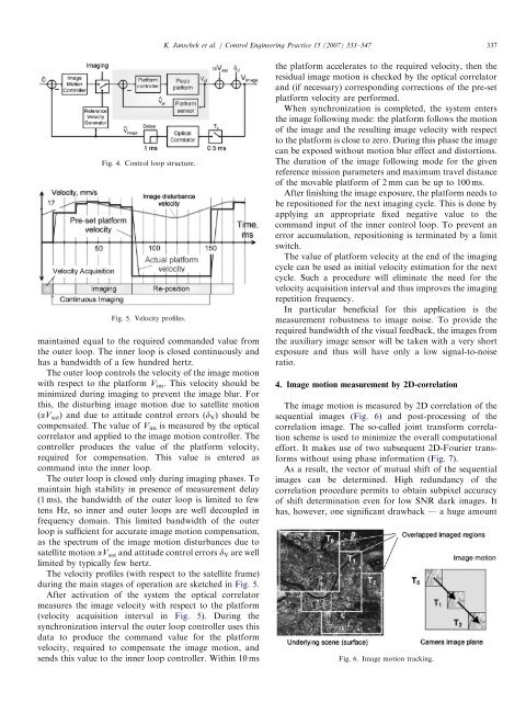
Fig. 5. Velocity pr<strong>of</strong>iles.<br />
maintained equal to the required commanded value from<br />
the outer loop. The inner loop is closed continuously and<br />
has a bandwidth <strong>of</strong> a few hundred hertz.<br />
The outer loop controls the velocity <strong>of</strong> the <strong>image</strong> motion<br />
with respect to the plat<strong>for</strong>m Vim. This velocity should be<br />
minimized during imaging to prevent the <strong>image</strong> blur. For<br />
this, the disturbing <strong>image</strong> motion due to satellite motion<br />
(aVsat) and due to attitude control errors (dV) should be<br />
compensated. The value <strong>of</strong> Vim is measured by the optical<br />
correlator and applied to the <strong>image</strong> motion controller. The<br />
controller produces the value <strong>of</strong> the plat<strong>for</strong>m velocity,<br />
required <strong>for</strong> compensation. This value is entered as<br />
command into the inner loop.<br />
The outer loop is closed only during imaging phases. To<br />
maintain high stability in presence <strong>of</strong> measurement delay<br />
(1 ms), the bandwidth <strong>of</strong> the outer loop is limited to few<br />
tens Hz, so inner and outer loops are well decoupled in<br />
frequency domain. This limited bandwidth <strong>of</strong> the outer<br />
loop is sufficient <strong>for</strong> accurate <strong>image</strong> motion compensation,<br />
as the spectrum <strong>of</strong> the <strong>image</strong> motion disturbances due to<br />
satellite motion aVsat and attitude control errors dV are well<br />
limited by typically few hertz.<br />
The velocity pr<strong>of</strong>iles (with respect to the satellite frame)<br />
during the main stages <strong>of</strong> operation are sketched in Fig. 5.<br />
After activation <strong>of</strong> the system the optical correlator<br />
measures the <strong>image</strong> velocity with respect to the plat<strong>for</strong>m<br />
(velocity acquisition interval in Fig. 5). During the<br />
synchronization interval the outer loop controller uses this<br />
data to produce the command value <strong>for</strong> the plat<strong>for</strong>m<br />
velocity, required to compensate the <strong>image</strong> motion, and<br />
sends this value to the inner loop controller. Within 10 ms<br />
ARTICLE IN PRESS<br />
K. Janschek et al. / Control Engineering Practice 15 (2007) 333–347 337<br />
the plat<strong>for</strong>m accelerates to the required velocity, then the<br />
residual <strong>image</strong> motion is checked by the optical correlator<br />
and (if necessary) corresponding corrections <strong>of</strong> the pre-set<br />
plat<strong>for</strong>m velocity are per<strong>for</strong>med.<br />
When synchronization is completed, the system enters<br />
the <strong>image</strong> following mode: the plat<strong>for</strong>m follows the motion<br />
<strong>of</strong> the <strong>image</strong> and the resulting <strong>image</strong> velocity with respect<br />
to the plat<strong>for</strong>m is close to zero. During this phase the <strong>image</strong><br />
can be exposed without motion blur effect and distortions.<br />
The duration <strong>of</strong> the <strong>image</strong> following mode <strong>for</strong> the given<br />
reference mission parameters and maximum travel distance<br />
<strong>of</strong> the movable plat<strong>for</strong>m <strong>of</strong> 2 mm can be up to 100 ms.<br />
After finishing the <strong>image</strong> exposure, the plat<strong>for</strong>m needs to<br />
be repositioned <strong>for</strong> the next imaging cycle. This is done by<br />
applying an appropriate fixed negative value to the<br />
command input <strong>of</strong> the inner control loop. To prevent an<br />
error accumulation, repositioning is terminated by a limit<br />
switch.<br />
The value <strong>of</strong> plat<strong>for</strong>m velocity at the end <strong>of</strong> the imaging<br />
cycle can be used as initial velocity estimation <strong>for</strong> the next<br />
cycle. Such a procedure will eliminate the need <strong>for</strong> the<br />
velocity acquisition interval and thus improves the imaging<br />
repetition frequency.<br />
In particular beneficial <strong>for</strong> this application is the<br />
measurement robustness to <strong>image</strong> noise. To provide the<br />
required bandwidth <strong>of</strong> the visual feedback, the <strong>image</strong>s from<br />
the auxiliary <strong>image</strong> sensor will be taken with a very short<br />
exposure and thus will have only a low signal-to-noise<br />
ratio.<br />
4. Image motion measurement by 2D-correlation<br />
The <strong>image</strong> motion is measured by 2D correlation <strong>of</strong> the<br />
sequential <strong>image</strong>s (Fig. 6) and post-processing <strong>of</strong> the<br />
correlation <strong>image</strong>. The so-called joint trans<strong>for</strong>m correlation<br />
scheme is used to minimize the overall computational<br />
ef<strong>for</strong>t. It makes use <strong>of</strong> two subsequent 2D-Fourier trans<strong>for</strong>ms<br />
without using phase in<strong>for</strong>mation (Fig. 7).<br />
As a result, the vector <strong>of</strong> mutual shift <strong>of</strong> the sequential<br />
<strong>image</strong>s can be determined. High redundancy <strong>of</strong> the<br />
correlation procedure permits to obtain subpixel accuracy<br />
<strong>of</strong> shift determination even <strong>for</strong> low SNR dark <strong>image</strong>s. It<br />
has, however, one significant drawback — a huge amount<br />
Fig. 6. Image motion tracking.