Linear Algebra II (pdf, 500 kB)

50
On the other hand,
φ φ ′ (f) n = φ
=
i=1
v ↦→
(w ∗ i ◦ f) ⊗ wi
n
i=1
w ∗ i (f(v))wi
=
n
i=1
v ↦→ w ∗ i
f(v) wi
= v ↦→ f(v) = f .
Now assume that V = W is finite-dimensional. Then by the above,
Hom(V, V ) ∼ = V ∗ ⊗ V
in a natural way. But Hom(V, V ) contains a special element, namely idV . What
is the element of V ∗ ⊗ V that corresponds to it?
12.14. Remark. Let v1, . . . , vn be a basis of V, and let v∗ 1, . . . , v∗ n be the basis of V ∗
dual to it. Then, with φ the canonical map from above, we have
n
φ
= idV .
i=1
v ∗ i ⊗ vi
Proof. Apply φ ′ as defined above to idV .
On the other hand, there is a natural bilinear form on V ∗ ×V , given by evaluation:
(l, v) ↦→ l(v). This gives the following.
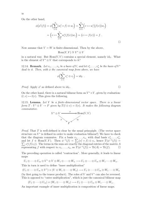
12.15. Lemma. Let V be a finite-dimensional vector space. There is a linear
form T : V ∗ ⊗ V → F given by T (l ⊗ v) = l(v). It makes the following diagram
commutative.
φ
V ∗ ⊗ V
T
F
Tr
Hom(V, V )
Proof. That T is well-defined is clear by the usual princpiple. (The vector space
structure on V ∗ is defined in order to make evaluation bilinear!) We have to check
that the diagram commutes. Fix a basis v1, . . . , vn, with dual basis v ∗ 1, . . . , v ∗ n,
and let f ∈ Hom(V, V ). Then φ −1 (f) =
i (v∗ i ◦ f) ⊗ vi, hence T (φ −1 (f)) =
i v∗ i (f(vi)). The terms in the sum are exactly the diagonal entries of the matrix A
representing f with respect to v1, . . . , vn, so T (φ −1 (f)) = Tr(A) = Tr(f).
The preceding operation is called “contraction”. More generally, it leads to linear
maps
U1 ⊗ · · · ⊗ Um ⊗ V ∗ ⊗ V ⊗ W1 ⊗ · · · ⊗ Wn −→ U1 ⊗ · · · ⊗ Um ⊗ W1 · · · ⊗ Wn .
This in turn is used to define “inner multiplication”
(U1 ⊗ · · · ⊗ Um ⊗ V ∗ ) × (V ⊗ W1 ⊗ · · · ⊗ Wn) −→ U1 ⊗ · · · ⊗ Um ⊗ W1 · · · ⊗ Wn
(by first going to the tensor product). The roles of V and V ∗ can also be reversed.
This is opposed to “outer multiplication”, which is just the canonical bilinear map
(U1 ⊗ · · · ⊗ Um) × (W1 ⊗ · · · ⊗ Wn) −→ U1 ⊗ · · · ⊗ Um ⊗ W1 · · · ⊗ Wn .
An important example of inner multiplication is composition of linear maps.