Lakshminarayan V. Chinta - Fields Institute - University of Toronto

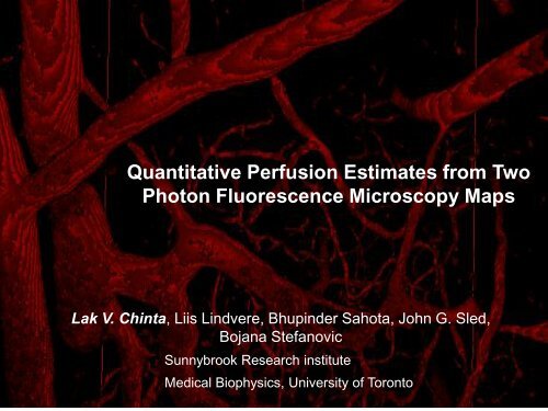
Quantitative Perfusion Estimates from Two
Photon Fluorescence Microscopy Maps
Lak V. Chinta, Liis Lindvere, Bhupinder Sahota, John G. Sled,
Bojana Stefanovic
Sunnybrook Research institute
Medical Biophysics, University of Toronto

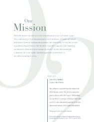
The Brain
1μm
capillary
neuron
astrocyte
microglia
2% total body weight
Consumes 20% O2 and 25% of glucose available to the body
Neurovascular Coupling:
Changes in neuronal activity are tightly coupled to changes in blood flow
and oxygenation

Neurovascular coupling
Brain Tissue
increased neuronal activity
Increased glial signaling
Increased metabolism demand
Mediators
Cerebral Vasculature
adaptation in flow, volume, and
oxygenation of the vascular bed
NO, GABA, 5HT, NE, DA, Ach, NPY, K+

Why neurovascular coupling is important?
• Many models of neurovascular coupling have been proposed.
- relating BOLD fMRI to neural activity seen on the millimeter scale
• Mechanisms underlying neurovascular coupling are not fully understood
- application of BOLD fMRI to the studies of stroke and brain diseases has had
limited scope
- the basic question is “what is the BOLD fMRI signal is measuring ?” or the lack of
detailed understanding of the neurovascular coupling at the micron level.
• No model exists at the micron level that can help in understanding the link
between neuronal and vascular 3D network state.
• Understanding neurovascular coupling at the micron scale will support:
- bottom-up modeling of BOLD fMRI signal
- platform for characterization of alterations in brain hemodynamics in disease

The Challenge
How do you quantitatively characterize neurovascular
coupling on the micron scale in vivo ?
Goal:
Quantitative estimation of cerebral hemodynamics at
the micron scale
- Cerebral blood flow (CBF) refers to volume per minute moving through
the vessels (nL/min)
- Perfusion refers to nutrient supply by the blood through the capillary bed
in the brain tissue (mL/g/min)

Fluorescent Dye
Temperature
Anesthetic
Animal preparation
Inter Cranial Pressure
Arterial Blood Pressure (ABP)
Blood Gas Analysis
1. Surgery under iso-flourane
2. Tracheotomy + mechanical ventilation
3. Cannulation of tail vein, femoral artery and vein
4. ICP recording via transducer placed inside
subarachnoid space of the spine (lumbar region)
5. Craniotomy over S1FL
6. Imaging under alpha-chloralose
7. IV administration of fluorescent dextran (Texas Red)
Breath Rate
Respiratory Pressure
End Tidal pCO 2
Electrical Stimulation
Heart Rate
O 2 Saturation
Sprague-Dawley rats (120-150g)
Imaging during:
a. Anatomical 3D image
following 33 mg/kg
bolus Texas red dextran
a. 2D time series of bolus
injection

Resolution:
~ 1μm lateral (x, y)
~ 3μm axial (z)
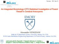
1% agarose
pial artery
2PFM Set-up
capillary bed
water immersion objective
cover glass
dental acrylic
skull
dura
pial vein
penetrating
arterioles
and venules
Adapted from - Kherlopian et al. BMC Systems Biology
2008 2:74

3D anatomical stacks acquisition
• Microvasculature clearly visible up to 600μm.
• Single 2D imaging plane is ~ 512 x 512 μm
• Lateral resolution 1μm and axial resolution 3 μm

2D bolus time series
• Single 2D imaging plane is ~ 250 x 250 μm
• ~ 50 μm below the cortical surface at 0.31 ± 0.07 fps
• Spatial resolution 1.59 μm/pixel

Analysis of perfusion estimation
• Estimation of transit time (TT) from the bolus time series.
• Identification of closed paths between vessels in the
FOV of the bolus tracking plane.
• Estimation of transit time in the individual segments
(multiple paths).
• Estimation of cerebral blood flow (CBF) and tissue
volume irrigated.

Transit time estimation from
bolus time series

Pre-processing of bolus time passage
bolus time series
vessels in FOV labeled
MIP
2D spatial median
filtering
t

Transit time estimation
• The signal intensity curves from bolus passage are
normalized and integrated over time.
• We model the bolus passage as a linear dynamical
process.

Second-order plus dead time model
(SOPDT)
• SOPDT model function (Rangiah et al. 2006) was used
to estimate damping ratio ( ), natural frequency ( ) and
dead time ( ).
• Laplace domain transfer functions
were then calculated:
G ( s )
G ( s )
s
6 2
2 2
t
2
e
s
n n
e
2 . 2 s
s 0 . 0 1 7 7 s
0 . 0 0 0 1

• Impulse response of the transfer functions was used to
calculate the onset time and peak time.
t ; t
Second-order plus dead time model
o p
t a n
1
n
1
1
2
2
(SOPDT)

Transit time estimation
• Transit time (normalized to earliest onset time) is
computed as
t t ( t t ) m i n ( t )
o p o
sec

Identification of closed paths
and estimation of TT in the
individual segments

Segmentation of the 3D vascular stacks
• Imaris (Bitplane Scientific Software) was used for semi-automated
segmentation of the 3D vascular network.
• Vertex-wise radii and x,y,z coordinates

Registration of bolus plane to the 3D
2D image plane from bolus tracking on
the 3D image
network
2D image plane from bolus tracking
on the 3D segmented image

Closed path identification
• Closed path identification between any two vessels of
the bolus tracking plane by tracing through the 3D
network.

Perfusion estimation – closed paths
• For direct closed paths, perfusion and CBF estimation is
can be computed easily
• CBF = CBV/TT (from the central volume principle)
• Perfusion = CBF/tissue volume irrigated

Perfusion estimation - multiple paths
• But, what if we have multiple connecting paths? How do
you estimate perfusion in these individual segments?

The problem in multiple paths
• We need to analyze the contributions of CBF in each of
the segments

Modeling CBF in individual segments
• We approach the problem by modeling CBF as current
flowing in a closed path.

TT estimation in individual segments
• We solve for the unknown transit time in the individual
segments based on equations of transit time and CBF.
3
t t t t t t t t t t t t t t
a b c d f g
t t t t t t t t t t t t t t
a b c e f g
e
a b c
1
c
3 9
3 9
C B V / t t C B V / t t C B V / t t
0
c c e e d d
f
d
e
d
g
9

Estimation of CBF and tissue
volume irrigated by the
individual segments

CBF estimation in individual segments
• We can compute CBF=CBV/TT (central volume
principle)
• CBF values coded in the individual segments
nL/min

Estimation of tissue volume irrigated
• For perfusion, we need the tissue volume irrigated by the
individual segments.
• Based upon the 2PFM literature, oxygen diffusion
distance in the rat’s somatosensory cortex is ~40-68 m
(Masamoto et al. 2007).
• Tissue volume irrigated can be estimated as a
convolution of ~65 μm sphere and our vascular subtree
centre lines.

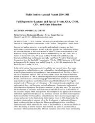
Perfusion estimation
mL/g/min
3.237
2.884
2.530
2.176
1.822
1.468
1.115
0.761
0.407
0.053
• Perfusion values are coded in the individual segments.
Z
600
500
400
300
200
100
0
400
300
200
Y
100
0
0
100
X
200
300
400

Heterogeneity in perfusion and CBF
~16.67% low mean perfusion 0.20 ± 0.02 mL/g/min
~61% physiological range 0.68 ± 0.29 mL/g/min
~19.44% mean perfusion 1.70 ± 0.38 mL/g/min
~2.74% perfusion value 3.23 mL/g/min

Heterogeneity in perfusion across rats
~7.4% low mean perfusion 0.16 ± 0.09 mL/g/min
~33.3% physiological range 0.64 ± 0.28 mL/g/min
~37.04% mean perfusion 1.72 ± 0.35 mL/g/min
~22.2% high mean perfusion 3.92 ± 1.24 mL/g/min
~11.76% low mean perfusion 0.18 ± 0.01 mL/g/min
~41.8% physiological range 0.68 ± 0.41 mL/g/min
~23.53% mean perfusion 1.77 ± 0.28 mL/g/min
~23.53% high mean perfusion 3.91 ± 1.83 mL/g/min

Perfusion estimation across modalities
• In the somatosensory cortex of rats under the same anesthesia
protocol
Optical Coherence Tomography (Boas 2010) ~0.51-0.68 mL/g/min
Iodo[14C]antipyrine autoradiographic studies (Nakao 2001) ~0.6 mL/g/min
• Our results show 48.7% of the segments within the physiological
range with median perfusion of 0.61 mL/g/min.

Conclusion
• Results show evidence of heterogeneity in perfusion: we
expect this heterogeneity to relate to local vascular
density.
• A novel methodology to estimate perfusion at the micron
level was developed: its application to a cohort of
subjects may relate cortical microvascular topology and
blood flow.
• Estimation of functional perfusion and CBF at the
micron scale.

Acknowledgements
• Supervisor: Bojana Stefanovic
• Collaborator: John G. Sled
• Lab
David Chartash
Simone Chaudhary
Adrienne Dorr
Eve Lake
Liis Lindvere
Martijn van Raaji
Bupinder Sahota
Andrew Stanisz
Kun Zhang
SiMing Zhang
• SRI (Neuro group)
• CIHR