Remote Sensing and Water management - FEFlow
Remote Sensing and Water management - FEFlow
Remote Sensing and Water management - FEFlow

Create successful ePaper yourself
Turn your PDF publications into a flip-book with our unique Google optimized e-Paper software.
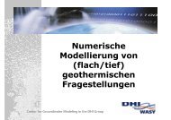
<strong>Remote</strong> <strong>Sensing</strong> <strong>and</strong><br />
Groundwater Modeling<br />
Institut für<br />
UmweltingenieurwissenschaftenIfU<br />
Wolfgang Kinzelbach<br />
Institute of Environmental Engineering<br />
ETH Zürich, Switzerl<strong>and</strong><br />
with<br />
Philip Brunner, Harrie-Jan Hendricks Franssen, Lesego Kgotlhang,<br />
Peter Bauer <strong>and</strong> Carmen Alberich
Contents<br />
Institut für<br />
UmweltingenieurwissenschaftenIfU<br />
• Data problems in groundwater modeling<br />
• Possible uses of remote sensing data in<br />
groundwater models with examples<br />
• Conclusions
Institut für<br />
UmweltingenieurwissenschaftenIfU<br />
Data problems of groundwater<br />
modelling<br />
• Data fields required: Recharge, transmissivity,<br />
leakage factor, evaporation rate, storage coefficient<br />
∂ h<br />
S = ∇( T∇ h) + q<br />
∂t<br />
• Only point values known, often few<br />
• Calibration usually not unique – predictive power<br />
poor<br />
• Reduction of number of degrees of freedom<br />
required (e.g. zonation, pivot points)
Typical problem<br />
Institut für<br />
UmweltingenieurwissenschaftenIfU<br />
• Fractured rock aquifer<br />
• Few boreholes<br />
• Recharge known to plus minus 1 order of magnitude<br />
• Storage coefficient known to plus minus 1 order of<br />
magnitude<br />
• Regional transmissivity known to plus minus 1 order of<br />
magnitude<br />
• Calibration non-unique<br />
• Management strategy unclear, worst case too pessimistic<br />
• Stop modelling or get new data!
Institut für<br />
UmweltingenieurwissenschaftenIfU<br />
Reduction of degrees of freedom<br />
Example recharge<br />
Recharge is a function of space <strong>and</strong> time<br />
Decompose in a spatial <strong>and</strong> a temporal factor<br />
<br />
Rxt ( , ) = gt ( ) f( xR ) average<br />
Time factor from lysimeters, spatial factor from<br />
l<strong>and</strong>use or data from remote sensing shown later<br />
Remains one degree of freedom: temporal <strong>and</strong><br />
spatial average
Institut für<br />
UmweltingenieurwissenschaftenIfU<br />
Physical interpolation from point<br />
data to areal distribution<br />
Example: Precipitation from METEOSAT<br />
Station data<br />
mm/a
Institut für<br />
UmweltingenieurwissenschaftenIfU<br />
Conditioning of stochastic models<br />
• Produce many equally likely realizations of the aquifer<br />
by the self-calibrating method<br />
• One source of observations maybe remote sensing fields<br />
• Set a term in the self-calibration procedure which<br />
penalizes the distance of the realization from data like<br />
the pattern obtained by remote sensing
Institut für<br />
UmweltingenieurwissenschaftenIfU<br />
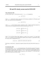
Types of remote sensing data<br />
• Frequency range in electromagnetic<br />
spectrum: visible, infrared, microwave<br />
(passive-active), radar<br />
• Resolution from cm to 500 km<br />
• Time sequence<br />
• Platform: satellite, airplane, balloon, tower<br />
• Geophysical remote sensing: magnetism,<br />
electromagnetic methods, gravity
Looking underground<br />
Institut für<br />
UmweltingenieurwissenschaftenIfU<br />
• Aeromagnetics (based on differences in magnetisation of<br />
rocks)<br />
– Structure: limits of aquifer<br />
– Intrusion dikes or fracture zones<br />
• Airborne Electromagnetics (TEM)<br />
– differences in electric conductivity from water (freshwater-saline<br />
water contrast),<br />
– or from lithology differences: e.g. clay versus s<strong>and</strong><br />
• Gravity variations in time<br />
– <strong>Water</strong> content (Storage term)<br />
– GRACE mission data
Institut für<br />
UmweltingenieurwissenschaftenIfU
Aeromag data Kanye<br />
Institut für<br />
UmweltingenieurwissenschaftenIfU
Institut für<br />
UmweltingenieurwissenschaftenIfU<br />
Lineaments from L<strong>and</strong>sat <strong>and</strong> aerial<br />
photography
Institut für<br />
UmweltingenieurwissenschaftenIfU<br />
Implementation of dikes in model<br />
Model without dikes Model with three classes of dikes
Institut für<br />
UmweltingenieurwissenschaftenIfU<br />
Thickness of Kalahari s<strong>and</strong> aquifer in the<br />
Okavango Delta
Magnetic depth (m)<br />
Institut für<br />
UmweltingenieurwissenschaftenIfU<br />
Calibration with ground truth<br />
400<br />
350<br />
300<br />
250<br />
200<br />
150<br />
100<br />
50<br />
0<br />
y = 0.9177x + 15.876<br />
R 2 = 0.9228<br />
0 50 100 150 200 250 300 350 400<br />
Borehole depth (m)<br />
Structural index<br />
N = 0.5
10 km<br />
Institut für<br />
UmweltingenieurwissenschaftenIfU<br />
Delineation of freshwater lenses in Okavango Delta<br />
with airborne TEM: Proxy for leakage factor
Institut für<br />
UmweltingenieurwissenschaftenIfU<br />
Looking at the surface elevation<br />
• DTM for depth to groundwater (evaporation<br />
from groundwater)<br />
• DTM for drainage patterns<br />
• Temporal differences in DTM indicate<br />
settling caused by cone of depression<br />
• DTM from radar satellites, shuttle<br />
topography mission, LIDAR altimetry
Institut für<br />
UmweltingenieurwissenschaftenIfU<br />
DTM from radar satellite images
Institut für<br />
UmweltingenieurwissenschaftenIfU<br />
DTM from radar satellite images
LIDAR Scan<br />
Institut für<br />
UmweltingenieurwissenschaftenIfU
Institut für<br />
UmweltingenieurwissenschaftenIfU<br />
Information related to areal recharge<br />
R= P−ET −ΔS−R • Determination of vegetation cover (NDVI)<br />
• Characterisation of l<strong>and</strong> use, l<strong>and</strong> use map (Optical range)<br />
• Soil map (Hyperspectral satellites)<br />
• Distribution of precipitation (weather radar, Meteosat)<br />
• Distribution of ET from energy balance
Precipitation<br />
sum of year 2000 from<br />
METEOSAT5 [mm/yr]<br />
Evapotranspiration<br />
over 24 hours<br />
ET 24 [mm d -1 ]<br />
from NOAA images<br />
via radiation<br />
energy balance<br />
Institut für<br />
UmweltingenieurwissenschaftenIfU
23.5 24.5<br />
- 17.5<br />
- 18.5<br />
Institut für<br />
UmweltingenieurwissenschaftenIfU<br />
10-year Average of Precipitation-ET (mm/yr)<br />
(from 97 images)
Institut für<br />
UmweltingenieurwissenschaftenIfU<br />
Recharge rates from chloride method („ground truth“)<br />
Recharge by Chloride<br />
Method (mm/yr)<br />
60 chloride samples from boreholes<br />
Average chloride concentration: 21 mg/l<br />
⇒ Average recharge: 6.8 mm/yr<br />
25.00<br />
20.00<br />
15.00<br />
10.00<br />
5.00<br />
0.00<br />
-5.00<br />
Chloride (mg/l)<br />
10000.0<br />
1000.0<br />
100.0<br />
10.0<br />
1.0<br />
y = 0.057x - 0.8448<br />
R 2 = 0.734<br />
0.1<br />
0 10 20 30 40 50 60<br />
Sample number<br />
-100 0 100 200 300 400<br />
Average Net Exchange (mm/yr)
Institut für<br />
UmweltingenieurwissenschaftenIfU<br />
Recharge distribution from combination<br />
Area with nonnegligible<br />
surface runoff<br />
Only for area where<br />
surface runoff is neglible<br />
(mm/a)
Institut für<br />
UmweltingenieurwissenschaftenIfU<br />
Conditioning of Stochastic Modelling<br />
Application to Kavimba Aquifer<br />
Data:<br />
• Transmissivities from pumping tests <strong>and</strong> variogram<br />
• Head observations<br />
• Digital terrain model<br />
• Recharge distribution from remote sensing plus its error<br />
from correlation analysis<br />
Two variants with 300 realizations each:<br />
• A: without using recharge distribution<br />
• B: with recharge distribution as conditioning data
Results:<br />
Application to Kavimba Aquifer<br />
Institut für<br />
UmweltingenieurwissenschaftenIfU<br />
Ensemble st<strong>and</strong>ard deviations of transmissivity, recharge <strong>and</strong> head<br />
Ensemble of realizations μ logT σ logT μ R σ R σ h<br />
A (without remote sensing<br />
information)<br />
B (with remote sensing<br />
information)<br />
-2.36 0.71 6.5 8.0 16.0<br />
-2.38 0.61 6.4 3.3 10.3<br />
Uncertainty reduction in input <strong>and</strong> output variables
Institut für<br />
UmweltingenieurwissenschaftenIfU<br />
Information related to surface waters<br />
• Determination of water covered area<br />
• Seasonal <strong>and</strong> permanent swamps<br />
• Change in ponding as measure for recharge<br />
• <strong>Water</strong> surface elevation, elevation changes<br />
• Using radar satellite information or<br />
optical/infrared satellite information
Institut für<br />
UmweltingenieurwissenschaftenIfU<br />
Observed water covered area<br />
NOAA AVHRR (optical, 5 b<strong>and</strong>s)<br />
- unsupervised classification<br />
9 June 2005<br />
Envisat ASAR (radar)<br />
- temporal variance <strong>and</strong> edge detection<br />
11 June 2005
Institut für<br />
UmweltingenieurwissenschaftenIfU<br />
Information related to soil<br />
• Mapping of salinity with multispectral data<br />
• Mapping of soil type (hyperspectral data)<br />
• Passive microwave for soil moisture<br />
• Infrared at night for soil temperatures
Institut für<br />
UmweltingenieurwissenschaftenIfU<br />
Mapping soil salinity with remote sensing<br />
Based on the spectrum of extremely saline pixels, a spectral match to<br />
that signature is defined :
GCP- conductivity (micrS/cm) j<br />
160000<br />
140000<br />
120000<br />
100000<br />
80000<br />
60000<br />
40000<br />
20000<br />
0<br />
Calibration with ground truth<br />
0 0.2 0.4 0.6 0.8 1<br />
Spectral match between GCP <strong>and</strong> Reference<br />
Institut für<br />
UmweltingenieurwissenschaftenIfU<br />
Non-irrigated<br />
areas<br />
Irrigated areas
The Yanqi Basin <strong>and</strong> its problems<br />
(due to doubling of population over the last 50 years)<br />
First Control<br />
Point Kaidu River<br />
Huang Shui River<br />
Qing Shui River<br />
Groundwater table rise due to irrigation<br />
Soil salinization<br />
Second<br />
Control Point<br />
Die-off of fish<br />
Kongque<br />
Drying up of „greenRiver corridor“<br />
Bostan<br />
Lake<br />
Decline of water level in lake<br />
Increase of salinity in lake
Institut für<br />
UmweltingenieurwissenschaftenIfU<br />
Method used to gain system underst<strong>and</strong>ing<br />
Coupled modeling of groundwater <strong>and</strong> surface water resources<br />
First layer of a two-layer model
Institut für<br />
UmweltingenieurwissenschaftenIfU<br />
ET in Yanqi basin year 2000 (mm/a)
Institut für<br />
UmweltingenieurwissenschaftenIfU<br />
Calibration of model using phreatic evaporation<br />
Model<br />
Using depthdependence<br />
from stable<br />
isotopes<br />
<strong>Remote</strong><br />
<strong>Sensing</strong><br />
Using ET,<br />
NDVI <strong>and</strong><br />
stable isotopes
Institut für<br />
UmweltingenieurwissenschaftenIfU<br />
Usefulness of remote sensing data<br />
• New data source for regional hydrology <strong>and</strong> water<br />
resources <strong>management</strong> especially in dry regions<br />
• Allowing step from point process to area<br />
• Mostly indirect data which only unfold their<br />
usefulness in connection with modelling<br />
(conditioning data, data assimilation)<br />
• Indispensable in regions with weak infrastructure<br />
<strong>and</strong> low accessibility<br />
• Great potential for improving quality of our work<br />
in the arid <strong>and</strong> semiarid environments
Institut für<br />
UmweltingenieurwissenschaftenIfU<br />
Problems with remote sensing data<br />
• Correlation to required information may be<br />
weak (noisy information)<br />
• Resolution problem<br />
• Availability of longer time series poor<br />
• Ground truth required <strong>and</strong> expensive<br />
• Clouds in optical <strong>and</strong> infrared window often<br />
crippling
Conclusions<br />
• The potential of remote sensing data in<br />
groundwater modelling is considerable<br />
Institut für<br />
UmweltingenieurwissenschaftenIfU<br />
• Data are indirectly related <strong>and</strong> therefore best used<br />
as conditioning data in a stochastic approach<br />
• Pattern information is more reliable than actual<br />
numbers<br />
• Ground truth is absolutely necessary<br />
• On the whole the new data sources have great<br />
potential to improve our work