Very Large SVM Training using Core Vector Machines

More documents

Recommendations

Info

ficult problems like NP-complete problems (Garey & Johnson, 1979), such “approximateness” has never been exploited in the design of SVM implementations. In this paper, we first transform the SVM optimization problem (with a possibly nonlinear kernel) to the minimum enclosing ball (MEB) problem in computational geometry. The MEB problem computes the ball of minimum radius enclosing a given set of points (or, more generally, balls). Traditional algorithms for finding exact MEBs do not scale well with the dimensionality d of the points. Consequently, recent attention has shifted to the development of approximation algorithms. Lately, a breakthrough was obtained by Bădoiu and Clarkson (2002), who showed that an (1 + ǫ)approximation of the MEB can be efficiently obtained using core-sets. Generally speaking, in an optimization problem, a core-set is a subset of the input points, such that we can get a good approximation (with an approximation ratio 1 specified by a user-defined ǫ parameter) to the original input by solving the optimization problem directly on the core-set. Moreover, a surprising property of (Bădoiu & Clarkson, 2002) is that the size of its core-set is independent of both d and the size of the point set. Inspired from this core-set-based approximate MEB algorithm, we will develop an approximation algorithm for SVM training that has an approximation ratio of (1 + ǫ) 2 . Its time complexity is linear in m while its space complexity is independent of m. The rest of this paper is organized as follows. Section 2 gives a short introduction on the MEB problem and its approximation algorithm. The connection between kernel methods and the MEB problem is given in Section 3. Section 4 then describes our proposed Core Vector Machine (CVM) algorithm. Experimental results are presented in Section 5, and the last section gives some concluding remarks. 2 MEB in Computational Geometry Given a set of points S = {x1, . . .,xm}, where each xi ∈ R d , the minimum enclosing ball of S (denoted MEB(S)) is the smallest ball that contains all the points in S. The MEB problem has found applications in diverse areas such as computer graphics (e.g., collision detection, visibility culling), machine learning (e.g., similarity search) and facility locations problems. 1 Let C be the cost (or value of the objective function) of the solution returned by an approximate algorithm, and C ∗ be the cost of the optimal solution. Then, the approximate algorithm “ has an approximation ratio ρ(n) for an input size n if C max C∗ , C∗ ” ≤ ρ(n). Intuitively, this measures how bad C the approximate solution is compared with the optimal solution. A large (small) approximation ratio means the solution is much worse than (more or less the same as) the optimal solution. Observe that ρ(n) is always ≥ 1. If the ratio does not depend on n, we may just write ρ and call the algorithm an ρ-approximation algorithm. Here, we will focus on approximate MEB algorithms based on core-sets. Let B(c, R) be the ball with center c and radius R. Given ǫ > 0, a ball B(c, (1 + ǫ)R) is an (1 + ǫ)-approximation of MEB(S) if R ≤ r MEB(S) and S ⊂ B(c, (1 + ǫ)R). A subset X ⊆ S is a core-set of S if an expansion by a factor (1 + ǫ) of its MEB contains S, i.e., S ⊂ B(c, (1+ǫ)r), where B(c, r) = MEB(X) (Figure 1). To obtain such an (1 + ǫ)approximation, Bădoiu and Clarkson (2002) proposed a simple iterative scheme: At the tth iteration, the current estimate B(ct, rt) is expanded incrementally by including the furthest point outside the (1 + ǫ)ball B(ct, (1 + ǫ)rt). This is repeated until all the points in S are covered by B(ct, (1 + ǫ)rt). Despite its simplicity, Bădoiu and Clarkson (2002) showed that the number of iterations, and hence the size of the final core-set, depends only on ǫ but not on d or m. εR R Figure 1: The inner circle is the MEB of the set of squares and its (1 + ǫ) expansion (the outer circle) covers all the points. The set of squares is thus a core-set. This independence of d is important on applying this algorithm to kernel methods (Section 3) as the kernel-induced feature space can be infinite-dimensional. As for the independence on m, it allows both the time and space complexities of our algorithm to grow slowly, as will be shown in Section 4.3. 3 MEB Problems and Kernel Methods Obviously, the MEB is equivalent to the hard-margin support vector data description (SVDD) (Tax & Duin, 1999), which will be briefly reviewed in Section 3.1. The MEB problem can also be used for finding the radius component of the radius-margin bound (Chapelle et al., 2002). Thus, as pointed out by Kumar et al. (2003), the MEB problem is useful in support vector clustering and SVM parameter tuning. However, we will show in Section 3.2 that other kernel-related problems, including the training of soft-margin one-class and two-class L2-SVMs, can also be viewed as MEB problems. 3.1 Hard-Margin SVDD Given a kernel k with the associated feature map ϕ, let the MEB in the kernel-induced feature space be B(c, R). The primal problem in the hard-margin SVDD is min R 2 The corresponding dual is : c − ϕ(xi) 2 ≤ R 2 , i = 1, . . . , m. (1) max α ′ diag(K) − α ′ Kα : 0 ≤ α, α ′ 1 = 1, (2)
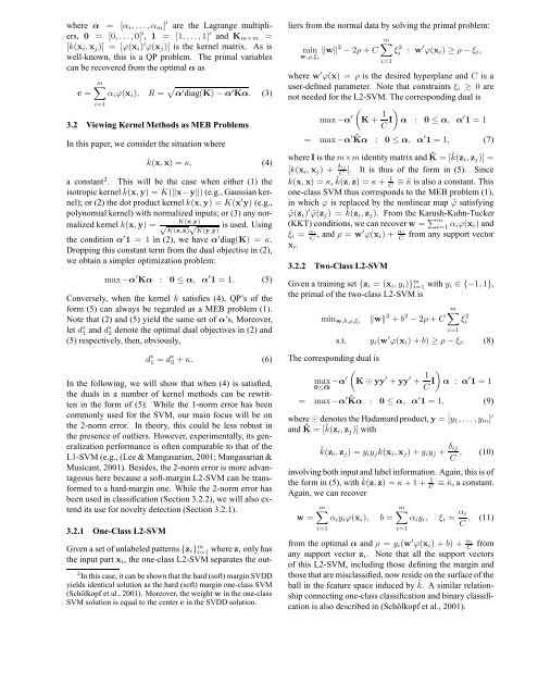
where α = [αi, . . .,αm] ′ are the Lagrange multipliers, 0 = [0, . . .,0] ′ , 1 = [1, . . . , 1] ′ and Km×m = [k(xi,xj)] = [ϕ(xi) ′ ϕ(xj)] is the kernel matrix. As is well-known, this is a QP problem. The primal variables can be recovered from the optimal α as c = m αiϕ(xi), R = α ′ diag(K) − α ′ Kα. (3) i=1 3.2 Viewing Kernel Methods as MEB Problems In this paper, we consider the situation where k(x,x) = κ, (4) a constant2 . This will be the case when either (1) the isotropic kernel k(x,y) = K(x−y) (e.g., Gaussian kernel); or (2) the dot product kernel k(x,y) = K(x ′ y) (e.g., polynomial kernel) with normalized inputs; or (3) any nor- K(x,y) malized kernel k(x,y) = √ K(x,x) √ K(y,y) is used. Using the condition α ′ 1 = 1 in (2), we have α ′ diag(K) = κ. Dropping this constant term from the dual objective in (2), we obtain a simpler optimization problem: max −α ′ Kα : 0 ≤ α, α ′ 1 = 1. (5) Conversely, when the kernel k satisfies (4), QP’s of the form (5) can always be regarded as a MEB problem (1). Note that (2) and (5) yield the same set of α’s, Moreover, let d∗ 1 and d∗2 denote the optimal dual objectives in (2) and (5) respectively, then, obviously, d ∗ 1 = d ∗ 2 + κ. (6) In the following, we will show that when (4) is satisfied, the duals in a number of kernel methods can be rewritten in the form of (5). While the 1-norm error has been commonly used for the SVM, our main focus will be on the 2-norm error. In theory, this could be less robust in the presence of outliers. However, experimentally, its generalization performance is often comparable to that of the L1-SVM (e.g., (Lee & Mangasarian, 2001; Mangasarian & Musicant, 2001). Besides, the 2-norm error is more advantageous here because a soft-margin L2-SVM can be transformed to a hard-margin one. While the 2-norm error has been used in classification (Section 3.2.2), we will also extend its use for novelty detection (Section 3.2.1). 3.2.1 One-Class L2-SVM Given a set of unlabeled patterns {zi} m i=1 where zi only has the input part xi, the one-class L2-SVM separates the out- 2 In this case, it can be shown that the hard (soft) margin SVDD yields identical solution as the hard (soft) margin one-class SVM (Schölkopf et al., 2001). Moreover, the weight w in the one-class SVM solution is equal to the center c in the SVDD solution. liers from the normal data by solving the primal problem: min w w,ρ,ξi 2 − 2ρ + C m ξ 2 i : w ′ ϕ(xi) ≥ ρ − ξi, i=1 where w ′ ϕ(x) = ρ is the desired hyperplane and C is a user-defined parameter. Note that constraints ξi ≥ 0 are not needed for the L2-SVM. The corresponding dual is max −α ′ K + 1 C I α : 0 ≤ α, α ′ 1 = 1 = max −α ′ ˜Kα : 0 ≤ α, α ′ 1 = 1, (7) whereI is the m×m identity matrix and ˜K = [ ˜ k(zi,zj)] = [k(xi,xj) + δij C ]. It is thus of the form in (5). Since k(x,x) = κ, ˜ k(z,z) = κ + 1 C ≡ ˜κ is also a constant. This one-class SVM thus corresponds to the MEB problem (1), in which ϕ is replaced by the nonlinear map ˜ϕ satisfying ˜ϕ(zi) ′ ˜ϕ(zj) = ˜ k(zi,zj). From the Karush-Kuhn-Tucker (KKT) conditions, we can recover w = m i=1 αiϕ(xi) and ξi = αi C , and ρ = w′ ϕ(xi) + αi C from any support vector xi. 3.2.2 Two-Class L2-SVM Given a training set {zi = (xi, yi)} m i=1 with yi ∈ {−1, 1}, the primal of the two-class L2-SVM is minw,b,ρ,ξi w 2 + b 2 − 2ρ + C The corresponding dual is max 0≤α −α′ m i=1 s.t. yi(w ′ ϕ(xi) + b) ≥ ρ − ξi. (8) K ⊙ yy ′ + yy ′ + 1 C I ξ 2 i α : α ′ 1 = 1 = max −α ′ ˜Kα : 0 ≤ α, α ′ 1 = 1, (9) where ⊙ denotes the Hadamard product, y = [y1, . . . , ym] ′ and ˜ K = [ ˜ k(zi,zj)] with ˜k(zi,zj) = yiyjk(xi,xj) + yiyj + δij , (10) C involving both input and label information. Again, this is of the form in (5), with ˜ k(z,z) = κ + 1 + 1 C ≡ ˜κ, a constant. Again, we can recover m m w = αiyiϕ(xi), b = αiyi, ξi = αi , (11) C i=1 i=1 from the optimal α and ρ = yi(w ′ ϕ(xi) + b) + αi C from any support vector zi. Note that all the support vectors of this L2-SVM, including those defining the margin and those that are misclassified, now reside on the surface of the ball in the feature space induced by ˜ k. A similar relationship connecting one-class classification and binary classification is also described in (Schölkopf et al., 2001).
Page 1: Very Large SVM Training using Core
Page 5 and 6: on using (10), (11) and αℓ = 0.
Page 7 and 8: CPU time (in seconds) 10 6 10 5 10

Very Large SVM Training using Core Vector Machines

You also want an ePaper? Increase the reach of your titles

Delete template?

Save as template?