Fox H functions in fractional diffusion - FRActional CALculus ...

More documents

Recommendations

Info

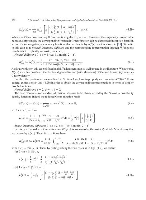
328 F. Mainardi et al. / Journal of Computational and Applied Mathematics 178 (2005) 321–331 K , (x) = 1 2,1 H3,3 x x (1, 1 − )(1, )(1, 2 ) (1, 1 − )(1, 1)(1, 2 ) , > . (4.2b) When = the corresponding H function is singular in z = x = 1. However, the singularity is removable because, surprisingly, the corresponding (reduced) Green function can be expressed (in explicit form) in terms of a (nonnegative) elementary function, that we denote by N (x), as it is shown in [21].We refer to this case as to neutral-fractional diffusion and the corresponding representation through H functions is redundant.Explicitly we write, for x>0, Neutral diffusion :0< = < 2; min{, 2 − }, K , := N 1 x (x) = −1 sin[(/2)( − )] 1 + 2x . (4.3) cos[(/2)( − )]+x2 As far as we know, this case of fractional diffusion seems not so well treated in the literature.We note that N (x) may be considered the fractional generalization (with skewness) of the well-known (symmetric) Cauchy density. For the other particular cases outlined in Section 3 we have to properly use properties (2.9)–(2.11) in general expressions (4.2a)–(4.2b) in order to obtain the corresponding representations in terms of simpler Fox H functions. Normal diffusion : = 2, = 1; = 0. The case of normal (or standard) diffusion is known to be characterized by the Gaussian probability density function.Indeed the reduced Green function reads K 0 1 2,1 (x) := D(x) = 2 √ exp(−x2 /4), x ∈ R, (4.4) so, for x>0, we have D(x) = 1 1 2x 2i +i∞ −i∞ (1 − s) (1 − s/2) xs ds = 1 1,0 H1,1 x 2 ( 1 2 , 1 2 ) . (4.5) (0, 1) Space-fractional diffusion:0< < 2, = 1;|| min{, 2 − }. In this case the reduced Green function K ,1 (x) is known to be the -strictly stable Lévy density that (x).Then, for x>0, we have we denote by L +i∞ K ,1 (x) := L 1 1 (x) = x 2i −i∞ (s/)(1 − s) ([( − )/2]s)(1 −[(− )/2]s) xs ds (4.6) with 0 < < min(, 1), Then, by distinguishing the two cases as in Eqs.(4.2), we obtain: (a) 0 < < 1;||, L 1 1,1 1 (1, 1)( (x) = H2,2 x − − 2 , 2 ) . (4.7a) (b) 1 < < 2;||2 − , x L 1 1,1 (x) = H2,2 ( 1 , 1 )(− 2 , − 2 ) (1 − 1 , 1 (0, 1)(1 − − 2 − − )(1 − 2 , 2 ) , − 2 ) . (4.7b)
F. Mainardi et al. / Journal of Computational and Applied Mathematics 178 (2005) 321–331 329 We note that it was Schneider [33], who first in 1986 has recognized that all stable probability densities can be represented in terms of Fox H functions. Previously, the stable (non-Gaussian) densities were known in general through their (convergent and asymptotic) series representations that in a few particular cases, { = 1 −1 3 , = 3 }, { = 1 −1 2 , = 2 }, { = 2 3 , = 0}, { = 3 2 , = 1 2 }, were interpreted in terms of known special functions.In his remarkable (but almost entirely neglected) article, Schneider has also pointed out the errors present in the literature for some of the above particular cases. More recently, the representation of the stable densities through Mellin–Barnes integrals has been exhaustively treated by a number of authors as in [36,21]. Time-fractional diffusion : = 2, 0 < < 2; = 0. In this case the reduced Green function K ,1 (x) is known to be a probability density with stretched exponential tails, that we denote (for historical reasons) by 1 2 M/2 where M/2 denotes a Wright-type function. 4 We thus write K 0 2, (x) := 1 2 M/2(x), (4.8) where, for x>0, M/2(x) = 1 x 1 +i∞ 2i −i∞ (1 − s) (1 − s/2) x s ds = H 1,0 1,1 x (1 − 2 , 2 ) (0, 1) with 0 < < 1. As a check we note that the simpler H function in (4.5) for the Gaussian density is recovered from (4.7a) in the limit = 2 and from (4.8)–(4.9) in the limit = 1. 4 The function M(z) is defined for any order ∈ (0, 1) and ∀z ∈ C by M(z) = ∞ n=0 (−z) n 1 = n![−n + (1 − )] ∞ n=1 (−z) n−1 (n) sin(n). (n − 1)! It turns out that M(z) is an entire function of order = 1/(1 − ), which provides a generalization of the Gaussian and of the Airy function.In fact, we obtain M1/2(z) = 1 √ exp(− z 2 /4), M1/3(z) = 3 2/3 Ai(z/3 1/3 ). M(z) is a special case of the Wright function ,(z).Originally, Wright [37–39] introduced and investigated the function ,(z) := ∞ n=0 zn , 0, z ∈ C, n!(n + ) with the restriction 0, in a series of notes starting from 1933 in the framework of the asymptotic theory of partitions.Only later, in 1940, he [40] considered the case −1 < < 0. We note that in the handbook of the Bateman Project, see [3], Vol.3, Ch. 18, presumably for a misprint, is restricted to be nonnegative.In his first analysis of the time fractional diffusion equation, Mainardi [17], aware of the Bateman project but not of the 1940 paper by Wright, introduced the two (Wright-type) auxiliary functions, F(z) := −,0(−z) and M(z) := −,1−(−z) with 0 < < 1, inter-related through F(z) = zM(z). For detailed information on the Wright-type functions (possibly related to time-fractional diffusion equations), the interested reader may consult e.g. [18–20,5,6,10,14]. (4.9)
Page 1 and 2: Journal of Computational and Applie
Page 3 and 4: F. Mainardi et al. / Journal of Com
Page 5 and 6: F. Mainardi et al. / Journal of Com
Page 7: F. Mainardi et al. / Journal of Com
Page 11: F. Mainardi et al. / Journal of Com

Fox H functions in fractional diffusion - FRActional CALculus ...

You also want an ePaper? Increase the reach of your titles

Delete template?

Save as template?