Stripe and ring artifact removal with combined wavelet — Fourier ...
Stripe and ring artifact removal with combined wavelet — Fourier ...
Stripe and ring artifact removal with combined wavelet — Fourier ...

You also want an ePaper? Increase the reach of your titles
YUMPU automatically turns print PDFs into web optimized ePapers that Google loves.
where the basis functions are orthogonal to each other, that is, the scalar product of every two<br />
Γn(t) meets<br />
〈Γn(t),Γm(t)〉 = <br />
<br />
1, ∀ n = m<br />
Γn(t) · Γm(t) =<br />
(2)<br />
0, ∀ n = m<br />
n<br />
Thereby, f(t) will be unequivocally represented by the coefficients an.<br />
The main motivation for the decomposition of a signal into orthogonal basis functions is the<br />
deployment of the original signal information into coefficient classes that specifically group<br />
interesting structural patterns. This aspect is particularly attractive for <strong>artifact</strong>s <strong>removal</strong> techniques.<br />
In addition, orthogonal transforms often yield coefficients, which become partly small<br />
or even zero. This characteristic of <strong>wavelet</strong> <strong>and</strong> <strong>Fourier</strong> analysis makes signal decomposition<br />
especially attractive for data compression purposes [22]. Moreover, the calculation of the coefficients<br />
an is very efficient <strong>and</strong> achieved in linear time o(N) by simple evaluation of scalar<br />
products:<br />
an = 〈 f(t),Γn(t)〉 (3)<br />
Furthermore, since <strong>Fourier</strong> <strong>and</strong> some <strong>wavelet</strong> transforms are separable, they can be applied<br />
successively for each dimension in the case of two or more dimensional signals.<br />
For the discrete <strong>Fourier</strong> transform (DFT), Γn(t) are sine <strong>and</strong> cosine functions at discrete<br />
frequencies wn = 2 · π · n, although the complex exponential notation Γn(t) = e −i·ωn·t is often<br />
preferred. In the <strong>Fourier</strong> domain, all structural information of a signal is entirely represented<br />
by frequencies, whereas any spatial information is completely distributed over the entire frequency<br />
range <strong>and</strong> thus hidden. In contrast, for the <strong>wavelet</strong> transform [23, 24, 25], Γn(t) are<br />
narrow groups of <strong>wavelet</strong>s of different sizes <strong>and</strong> frequencies <strong>and</strong> both, spatial <strong>and</strong> frequency<br />
information is retained. For the discrete <strong>wavelet</strong> transform (DWT), a variety of <strong>wavelet</strong> types<br />
exist, which allow perfect reconstruction of the original signal, in particular the Daubechies<br />
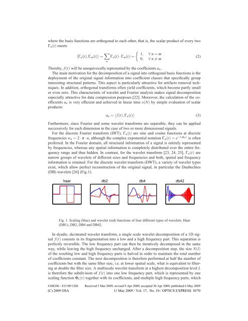
(DB) <strong>wavelet</strong>s [26] (Fig.1).<br />
haar db2 db4 db42<br />
Fig. 1. Scaling (blue) <strong>and</strong> <strong>wavelet</strong> (red) functions of four different types of <strong>wavelet</strong>s: Haar<br />
(DB1), DB2, DB4 <strong>and</strong> DB42.<br />
In dyadic, decimated <strong>wavelet</strong> transform, a single scale <strong>wavelet</strong> decomposition of a 1D signal<br />
f(t) consists in its fragmentation into a low <strong>and</strong> a high frequency part. This separation is<br />
perfectly reversible. The low frequency part can then be iteratively decomposed in the same<br />
way, while leaving the high frequency unchanged. After a decomposition step, the size N(l)<br />
of the resulting low <strong>and</strong> high frequency parts is halved in order to maintain the total number<br />
of coefficients constant. The next decomposition is therefore performed at half the number of<br />
coefficients but <strong>with</strong> the same filter size, i.e. at lower spatial scale, what is equivalent to filte<strong>ring</strong><br />
at double the filter size. A multiscale <strong>wavelet</strong> transform at a highest decomposition level L<br />
is therefore the subdivision of f(t) into one low frequency part, which is represented by one<br />
scaling function ΦL(t) together <strong>with</strong> its coefficients, <strong>and</strong> multiple high frequency parts, which<br />
#108296 - $15.00 USD Received 5 Mar 2009; revised 9 Apr 2009; accepted 30 Apr 2009; published 6 May 2009<br />
(C) 2009 OSA 11 May 2009 / Vol. 17, No. 10 / OPTICS EXPRESS 8570