Entire volume - Eawag
Entire volume - Eawag
Entire volume - Eawag

Create successful ePaper yourself
Turn your PDF publications into a flip-book with our unique Google optimized e-Paper software.
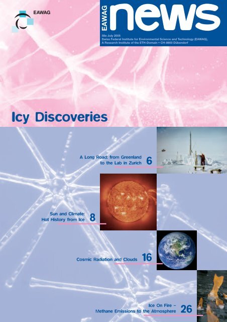
EAWAG<br />
news<br />
58e July 2005<br />
Swiss Federal Institute for Environmental Science and Technology (EAWAG),<br />
A Research Institute of the ETH-Domain • CH-8600 Dübendorf<br />
EAWAG<br />
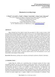
Icy Discoveries<br />
Sun and Climate:<br />
Hot History from Ice 8<br />
A Long Road: from Greenland<br />
to the Lab in Zurich 6<br />
Cosmic Radiation and Clouds 16<br />
Ice On Fire –<br />
Methane Emissions to the Atmosphere 26
EAWAG news 58e • July 2005<br />
Information Bulletin of the EAWAG<br />
Publisher Distribution and © by:<br />
EAWAG, P.O. Box 611, CH-8600 Dübendorf<br />
Phone +41 (0)44 823 55 11<br />
Fax +41 (0)44 823 53 75<br />
http://www.eawag.ch<br />
Editor Martina Bauchrowitz, EAWAG<br />
Translations EnviroText, Zürich<br />
Linguistic revision David Livingstone, EAWAG<br />
Figures Peter Nadler, Küsnacht; Lydia Zweifel, EAWAG;<br />
Copyright Reproduction possible on request.<br />
Please contact the editor.<br />
Publication 2–3 times per year in English, German and<br />
French. Chinese edition in cooperation with INFOTERRA<br />
China National Focal Point.<br />
Cover Photos M. Märki and J. Beer, EAWAG; NASA;<br />
Research Center Ocean Margins, Bremen<br />
Design inform, 8005 Zurich<br />
Layout Peter Nadler, 8700 Küsnacht<br />
Printed on original recycled paper<br />
Subscriptions and changes of address<br />
New subscribers are welcome! Please contact<br />
martina.bauchrowitz@eawag.ch<br />
ISSN 1440-5289<br />
EAWAG<br />
Icy Discoveries<br />
2 An Icy Look Back to the Future<br />
Lead Article<br />
3 Ice and Climate<br />
Research Reports<br />
6 A Long Road: from Greenland to the<br />
Lab in Zurich<br />
8 Sun and Climate: Hot History from<br />
Cool Ice<br />
11 Why Did a Cold Period Follow on the<br />
Heels of the Last Ice Age?<br />
14 The Compass in the Ice<br />
16 Cosmic Radiation and Clouds<br />
19 Ice Cover on Lakes and Rivers<br />
23 The North Atlantic Oscillation<br />
26 Ice On Fire – Methane Emissions to<br />
the Atmosphere<br />
In Brief<br />
29 Publications<br />
36 In Brief<br />
An Icy Look<br />
Back to the Future<br />
Martina Bauchrowitz,<br />
Editor<br />
Imagine you have arranged to meet some<br />
friends at a cinema. You are delayed unexpectedly<br />
and don’t arrive till an hour after<br />
the film has started. Just as you are getting<br />
comfortable in your seat and getting into the<br />
story, the film tears, and the screening has<br />
to be cancelled. You are very disappointed,<br />
since you would love to know how the film<br />
turns out. What can you do? You could<br />
perhaps try to guess how the story continues<br />
on the basis of the short snippet you<br />
have seen yourself, extended by what your<br />
friends can remember. Of course, the descriptions<br />
of your friends are nowhere near<br />
as detailed as your own experience, but<br />
have the advantage that they cover a far<br />
longer part of the film. In any case, your prediction<br />
of how the film continues is just a<br />
guess.<br />
This is how it is for scientists when they attempt<br />
to piece together via computer models<br />
a picture of how the earth’s climate might<br />
develop in the future. The more information<br />
that is available to put into the model, the<br />
more reliable the predictions will be. Climate<br />
researchers can fall back on databases of<br />
climate-relevant factors accumulated from<br />
a broad range of precise recent observations<br />
and instrumental measurements.<br />
These include air temperatures, the exact<br />
timing of the break-up of lake ice in spring,<br />
solar activity, and the degree of glaciation<br />
of the earth. Two articles in this edition of<br />
EAWAG news analyze historical records of<br />
lake ice cover, such as those that have been<br />
kept for the Lej da San Murezzan (the Lake<br />
of St. Moritz) since 1832. In terms of our film,<br />
these recent climate markers correspond to<br />
the part of the film you saw in person.<br />
In addition, climate researchers also examine<br />
the various natural archives that have<br />
been left behind as silent witnesses to the<br />
beginnings of the history of our climate. In<br />
particular, the polar ice caps contain valuable<br />
information on thousands of years of<br />
past climate conditions. In the international<br />
“Greenland Ice Core Project”, in which<br />
EAWAG participated, a 3-km-long ice core,<br />
10 cm in diameter, was drilled out of the<br />
Arctic ice shield between 1990 and 1992. It<br />
contains precipitation from the last 100 000<br />
years. Meter for meter and ice layer for ice<br />
layer, these ice cores have been carefully<br />
examined over the past 12 years. EAWAG<br />
alone has worked on thousands of ice core<br />
samples. Some of the results you will find in<br />
this current issue of EAWAG news.<br />
A further factor which climate researchers<br />
might find relevant is the behavior of<br />
methane hydrate. This ice-like compound,<br />
which is found, for instance, in deep sea<br />
sediments, is composed of water and methane<br />
and is formed at low temperatures and<br />
high pressure. It is estimated that around<br />
10 000 billion tonnes of methane in the form<br />
of this gas hydrate are sitting on the beds of<br />
the world’s oceans. Given this enormous<br />
quantity, concern is growing that “frozen”<br />
methane will escape, enter the atmosphere,<br />
add to the greenhouse effect, and thereby<br />
accelerate climate change. An EAWAG research<br />
group is therefore also involved in investigating<br />
the behavior of methane hydrate<br />
on the seabed.<br />
Ice in various forms therefore supplies much<br />
valuable information about present and past<br />
environmental conditions. Our only chance<br />
of obtaining reasonably reliable predictions<br />
of the climate of the future depends on our<br />
success in using this information to reconstruct<br />
the beginning of the climate film.<br />
EAWAG news 58 2
Ice and Climate<br />
About 80% of all the fresh water in the world is trapped as ice in<br />
the two polar regions. This ice is an exceptionally good environmental<br />
archive, containing invaluable clues to hundreds of thousands<br />
of years of climate history. Information on past climate can<br />
also be obtained from analyses of historical records of lake ice<br />
cover, such as those from the Lej da San Murezzan (the Lake of<br />
St. Moritz) in Switzerland and Lake Baikal in Siberia. A somewhat<br />
puzzling substance, which looks like ice, is methane hydrate. It<br />
normally lies buried in the deep-sea sediment, but slight changes<br />
in environmental conditions could cause it to rise to the sea surface,<br />
in which case it would be possible for large amounts of the<br />
greenhouse gas methane to enter the atmosphere, resulting in a<br />
serious acceleration of climate warming.<br />
Water conjures up images of babbling<br />
brooks and deep blue lakes reflecting snowcapped<br />
peaks. But water comes in other<br />
states, for example as a gas, when it is<br />
evaporated and transported from the sea<br />
onto the land, or as a solid, as snow and<br />
ice, when the temperature falls below zero.<br />
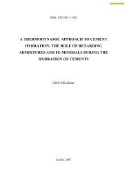
Considering all three states, most of us<br />
would be surprised to hear that most of the<br />
fresh water on the earth today is not found<br />
in rivers and lakes, but as ice (Fig. 1).<br />
Almost all of this frozen water – 99.4% –<br />
is located in the polar regions; i.e., in Antarctica<br />
and Greenland. The Antarctic ice mass<br />
is in parts 5 km thick, while in Greenland the<br />
ice depth can reach 3 km. The amount of ice<br />
in glaciers at lower latitudes accounts for<br />
only 0.6% of the total, and this proportion is<br />
unfortunately continually decreasing.<br />
Ice is, however, more than just frozen water.<br />
It provides us with a lot of invaluable information<br />
about current and past changes in<br />
the environment. Much of what was once<br />
trapped under the ice is just waiting to be<br />
brought out and investigated [1].<br />
Ice as an Archive<br />
There is practically nothing that does not<br />
leave a long-term record in the ice. But how<br />
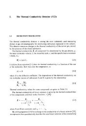
does ice become such an archive? Land ice<br />
derives from snow. Freshly fallen snow is<br />
quite soft and light and contains about 90%<br />
air (Fig. 2). Within just a few days the ice<br />
crystals condense to firn, which, under the<br />
3 EAWAG news 58<br />
pressure of new snow layers, becomes<br />
harder and denser, until at a certain depth<br />
the firn crystals fuse to form ice (Fig. 3).<br />
Snow and ice, though, consist not just of<br />
water. As clouds form, atmospheric water<br />
vapor condenses most readily around<br />
aerosol particles, which can contain a wide<br />
variety of chemical substances. In addition,<br />
as a snow flake wafts down to earth, it can<br />
pick up a number of substances from the<br />
air. And finally, all sorts of things settle on<br />
freshly fallen snow: pollen and fine dust from<br />
volcanoes or deserts, for instance, as well<br />
as larger, more spectacular finds such as the<br />
stone-age man Ötzi or ice-age mammoths.<br />
The fact that all these environmental samples<br />
have been stored at very low temperatures<br />
is one of the main reasons that makes<br />
Groundwater and<br />
soil moisture<br />
22.4%<br />
Lakes and rivers<br />
0.6%<br />
Ice<br />
77%<br />
Fig. 1: Distribution of global fresh water. Water vapor<br />
in the atmosphere, which accounts for only 0.04% of<br />
the total, is not included.<br />
ice such an exceptional environmental<br />
archive [2].<br />
The GRIP Ice Core<br />
Drilling in the polar ice sheet places high<br />
demands on both drilling techniques and<br />
logistics. Setting up a drill camp and conducting<br />
a drilling operation at 3000 –4000 m<br />
above sea level more than a thousand kilometers<br />
from the nearest town during several<br />
summers is really only possible within the<br />
framework of an international operation. The<br />
first deep-drilling operations to reach the<br />
Snow<br />
Ice<br />
granulate<br />
Firn<br />
Glacial ice<br />
90% air<br />
50% air<br />
20–30% air<br />
Melting and<br />
calving<br />
Iceberg<br />
Ice flow<br />
Bedrock<br />
Drill site<br />
Snow<br />
Fig. 3: Cross-section of the polar ice sheet. In the higher parts of the ice sheet, ice is being continually formed<br />
from snow. This ice flows slowly towards the coast, where it melts or floats off into the sea as icebergs (a process<br />
known as “calving”). This flow of ice means that the annual ice layers become thinner with increasing depth.<br />
bedrock under the ice sheet were carried<br />
out as long as 40 years ago. Since then<br />
there have been about a dozen similar projects.<br />
One of the latest large drilling campaigns<br />
was the Greenland Ice Core Project<br />
(GRIP) in central Greenland. From 1990 to<br />
1992, scientists from Belgium, Denmark,<br />
Germany, the UK, France, Iceland, Italy and<br />
Switzerland drilled an ice core 3029 m long<br />
and 10 cm in diameter which contains precipitation<br />
from the last 100,000 years.<br />
Lengthy discussions ensued to determine<br />
the best possible way of dividing up the<br />
ice between the various research groups in<br />
order to cover the up to 50 different parameters<br />
to be investigated, ranging from ice<br />
structures, isotopes, and various chemical<br />
substances, to dust and volcanic ash. This<br />
“squaring of the circle” was made all the<br />
harder since a certain part of the core had to<br />
be reserved for possible later verifications<br />
and additional parameters.<br />
For the drilling operation, a custom-made<br />
electrically driven mechanical drill bit was<br />
used. Using a steel cable, this was lowered<br />
into the borehole, where it could drill a core<br />
section up to 2.5 m long. To prevent the<br />
borehole from slowly closing under the<br />
enormous pressure of the ice, it was filled<br />
with a liquid which does not freeze even at<br />
–30 °C (the annual mean temperature at the<br />
drill site), and has the same density as ice.<br />
The drill bit was then brought back to the<br />
surface and the core removed. After being<br />
measured and numbered, each piece was<br />
given a preliminary examination and the first<br />
samples were removed. Finally, the cores<br />
were cut with a bandsaw into sections<br />
55 cm in length, packed into plastic bags<br />
in well-insulated styrofoam boxes, and prepared<br />
for the flight to Copenhagen. There<br />
they were cut up according to the distribu-<br />
tion plan and forwarded to the respective<br />
research groups for analysis.<br />
Cosmogenic Radionuclides<br />
in Ice<br />
Amongst other things, EAWAG is interested<br />
in the radionuclide beryllium-10 ( 10Be) contained<br />
in the GRIP ice cores. This radioactive<br />
isotope of the element beryllium is<br />
formed continually in the atmosphere, and<br />
falls to the ground in precipitation (see box).<br />
Nonetheless, the rate of production of these<br />
cosmogenic radionuclides in the atmosphere<br />
is relatively low: on average, only<br />
around 1 million 10Be atoms per year fall on<br />
each cm2 of the earth’s surface. It is therefore<br />
not surprising that extremely sensitive<br />
instruments, called accelerator mass spectrometers,<br />
are required for their detection.<br />
This instrument is capable of detecting and<br />
counting individual atoms (see article by<br />
S. Bollhalder and I. Brunner on p. 6).<br />
Reconstruction of the Past<br />
Climate<br />
Why go to such expense just to count a few<br />
10Be atoms? The main reason is that by do-<br />
Origin of Cosmogenic Radionuclides<br />
ing this we can learn something about past<br />
variations in solar activity and in the strength<br />
of the earth’s magnetic field. The rate of production<br />
of 10Be atoms in the atmosphere is<br />
not constant and depends, for instance, on<br />
the solar activity [3]. The cosmic radiation<br />
that is responsible for the production of<br />
10Be in the atmosphere originates from our<br />
galaxy, which consists of around 100 billion<br />
stars similar to our sun. When the cosmic<br />
radiation approaches our solar system, it<br />
first encounters the heliosphere, a spherically<br />
shaped region around the sun with a<br />
radius of about 15 billion kilometers. The<br />
heliosphere consists of ionized gas, known<br />
as the solar wind, which streams away from<br />
the sun at high speed. The solar wind carries<br />
with it the sun’s magnetic field, and<br />
because of this it shields the earth’s atmosphere<br />
to a certain extent from the cosmic<br />
radiation (Fig. 4), thus reducing the production<br />
rate of 10Be. In other words, the more<br />
active the sun is, the lower the 10Be count.<br />
This provides us with a complicated but<br />
unique method of learning about the history<br />
of the sun and its variability (see articles by<br />
M. Vonmoos on p. 8 and R. Muscheler on<br />
p. 11). The 10Be data also allowed us to test<br />
a hypothesis proposed by Danish scientists<br />
at the end of the 1990s which asserts that<br />
the cosmic radiation influences the climate<br />
(see article by J. Beer on p. 16).<br />
In addition, the rate of production of 10Be is<br />
influenced by the earth’s magnetic field. The<br />
Cosmogenic radionuclides originate through processes which the alchemists in the Middle<br />
Ages tried in vain to imitate: namely through the transmutation of elements; e.g., from nitrogen<br />
to beryllium or from argon to chlorine. What the alchemists did not manage to do, nature does<br />
at will. Cosmic radiation, consisting of high-energy particles (protons and helium nuclei), penetrate<br />
the earth’s atmosphere, colliding there with the oxygen, nitrogen and argon atoms of the<br />
air. This results in whole cascades of new particles, including neutrons, which likewise collide<br />
with other atoms, breaking them in turn into smaller particles. Most of the collision products<br />
are unstable and are immediately transformed into stable isotopes which can no longer be distinguished<br />
from those present beforehand. However, 10 Be and 36 Cl remain unchanged for long<br />
periods, due to their long half-lives of 1.5 million and 301,000 years, respectively. After an average<br />
residence time in the atmosphere of about 1 year, most of these isotopes are transported<br />
to earth in the precipitation. If a 10 Be atom found a snowflake for this journey, it is possible that<br />
it could end up in a glacier or in a polar ice sheet.<br />
EAWAG news 58 4
Fig. 4: The magnetic field of the solar wind interacts with the magnetic field of the earth. Together they form a natural<br />
protective shield which lowers the amount of cosmic radiation from outer space reaching the earth’s atmosphere.<br />
magnetic field lines, which span the earth<br />
from pole to pole, only permit the charged<br />
particles of the cosmic radiation to enter<br />
the earth’s atmosphere when these have<br />
sufficient energy (more precisely, momentum<br />
per unit charge). The stronger the magnetic<br />
field, the more effectively it shields the<br />
earth from cosmic radiation, resulting in<br />
lower rates of production of 10Be. Analyses<br />
of volcanic rock and sediments show that<br />
the earth’s magnetic field has clearly varied<br />
over the past millennia. As expected, these<br />
fluctuations were recorded in the ice and<br />
can be reconstructed (see article by J. Beer<br />
on p. 14).<br />
Ice Cover as a Climate<br />
Parameter<br />
Ice provides not only a valuable record of<br />
solar activity and the magnetic field. Further<br />
information about the climate can be<br />
gleaned from historical records of lake ice<br />
cover (see article by D. Livingstone on<br />
p. 19). For example, the calendar date of<br />
freeze-up of Lake Suwa in Japan has been<br />
documented almost continuously since<br />
1443. This unique data set has been used in<br />
many historical climatological studies of the<br />
North Pacific region. The longest data set<br />
from a Swiss lake is that of the calendar date<br />
of ice break-up on Lej da San Murezzan,<br />
which dates back to 1832. A further investigation<br />
pursued the question of whether<br />
there is a connection between the ice cover<br />
of lakes and the North Atlantic Oscillation<br />
(see article by D. Livingstone on p. 23). The<br />
North Atlantic Oscillation is a “see-saw” in<br />
surface atmospheric pressure between the<br />
5 EAWAG news 58<br />
Azores High and the Iceland Low. In winter,<br />
it results in variations in the strength of the<br />
westerly winds that transport relatively<br />
warm, moist, maritime air eastwards over<br />
Europe. These variations result in corresponding<br />
variations in the severity of winter<br />
in Europe and much of central Asia, which<br />
are reflected in the timing of thawing of ice<br />
on lakes in these regions [4].<br />
Ice from Methane Hydrate<br />
And lastly, we leave ice as a tracer of past<br />
climate and turn to methane hydrate. This is<br />
a compound of ice (i.e., water) and methane.<br />
It is formed at low temperatures and high<br />
pressure – e.g., in deep sea sediments –<br />
and is stable only under such conditions.<br />
The joint project CRIMEA involves an international<br />
group of scientists, including scientists<br />
from EAWAG, who are attempting to<br />
answer the question of whether this methane<br />
hydrate represents a danger to our<br />
environment (see article by C. Schubert on<br />
p. 26). Even a minor change in environmental<br />
conditions – such as a slight increase in<br />
the temperature of the deep-sea water or a<br />
shift in pressure due to sea level variations<br />
– could lead to methane hydrate being released<br />
and decomposing. This could result<br />
in large quantities of methane reaching<br />
the atmosphere. Since methane is one of<br />
the most important greenhouse gases after<br />
carbon dioxide, the consequences for the<br />
climate could be severe [5].<br />
Looking Back to the Future<br />
To predict the future has always been a<br />
dream of mankind. While earlier prophets<br />
were not particularly successful with reading<br />
cards and tea leaves, scientists today<br />
attempt to divine the future climate using<br />
sophisticated computer models. Such computer<br />
models only provide reliable results if<br />
all of the significant processes and their<br />
interactions are correctly parameterized. In<br />
addition, they have to be studied on a sufficiently<br />
long timescale. We can only hope to<br />
foresee future climate change if we are able<br />
to understand past climate changes. A good<br />
prophet therefore takes a long hard look at<br />
the past.<br />
Jürg Beer, physicist and leader<br />
of the Radioactive Tracers group<br />
in the Department of Surface<br />
Waters, is a titular professor at<br />
ETH Zurich. Research area: cosmogenic<br />
radionuclides; effect of<br />
solar activity on the climate.<br />
[1]Bradley R.S. (1985): Climate and climate variability.<br />
In: Quaternary Paleoclimatology – Methods of Paleoclimatic<br />
Reconstruction (ed. R.S. Bradley). Allen and<br />
Unwin, Boston, p. 11–46.<br />
[2] Beer J. (1995): Climate information from polar ice<br />
cores. EAWAG news 38e, 3–5.<br />
[3] Beer J., Mende W., Stellmacher R. (2000): The role<br />
of the Sun in climate forcing. Quaternary Science Reviews<br />
19, 403–415.<br />
[4] Straile D., Livingstone D.M., Weyhenmeyer G.A.,<br />
George D.G. (2003): The response of freshwater ecosystems<br />
to climate variability associated with the Nord<br />
Atlantic Oscillation. In: The North Atlantic Oscillation –<br />
Climatic Significance and Environmental Impact (ed.<br />
J.W. Hurrell). American Geophysical Union, Washington,<br />
p. 263–279.<br />
[5] Kvenvolden K.A. (1988): Methane hydrates and global<br />
climate. Global Biogeochemical Cycles 2, 221–229.
A Long Road: from Greenland<br />
to the Lab in Zurich<br />
Conclusions can be drawn about past environmental changes<br />
from telltale footprints left in environmental records. We are following<br />
one such hot lead in our investigations of the 3-km-long<br />
Greenland ice core. Layer for layer, the ice is examined to determine<br />
the concentrations of the radionuclide beryllium-10 ( 10 Be).<br />
From such data it is possible to obtain information about past<br />
climate changes. About 10,000 ice samples have been prepared<br />
by the EAWAG laboratory in recent years for measurement in the<br />
ETHZ/PSI accelerator mass spectrometer.<br />
Each year, rain and snow transport around<br />
1 million atoms of the radionuclide beryllium-10<br />
( 10Be) from the atmosphere on to<br />
each square cm of the earth’s surface. Some<br />
of these 10Be atoms are frozen, layer by<br />
layer, into the polar ice. Taking the global<br />
annual mean precipitation to be 1 m, this<br />
means that 1 kg of ice contains approximately<br />
10 million 10Be atoms. At first glance<br />
this would appear to be many. 10 million<br />
10Be atoms, though, weigh just 10 –15 g, the<br />
equivalent of a single raindrop in Lake Constance.<br />
To detect such a low concentration<br />
is a challenge to analytical science. To keep<br />
pace with the development of the accelerator<br />
mass spectrometer, over the last 15<br />
years EAWAG has developed an elegant<br />
sample preparation method (see box). This<br />
article provides an insight into the routine<br />
work carried out in our laboratory and de-<br />
Extraction and Detection of 10 Be<br />
scribes how 10Be atoms are extracted from<br />
the ice core and prepared for measurement<br />
in the ETHZ/PSI accelerator mass spectrometer<br />
at Hönggerberg, Zurich.<br />
From the Arctic to the<br />
EAWAG Laboratory<br />
The ice cores from Greenland (55-cm-long<br />
sections, maximum a quarter of the total<br />
cross section) are sealed in plastic bags and<br />
packed in styrofoam boxes before being<br />
sent to Dübendorf, where they are stored in<br />
a refrigerated room at –20 °C until required<br />
for preparation (Photo 1). Some of the ice<br />
samples are cut to smaller size with a bandsaw<br />
(Photo 2) to obtain a higher temporal<br />
resolution. Prior to the actual preparation<br />
procedure, each sample is washed with high<br />
purity water to remove any residual bore<br />
fluid and other external contaminants. Final-<br />
Traditionally, radionuclides are detected by means of their radioactive decay. However, this<br />
method is only of use if the radionuclide being investigated has a sufficiently short half-life.<br />
Within a reasonable measuring period – several days to several weeks at most – enough atoms<br />
have to decay so that they can be detected without excessive measuring error. It is precisely<br />
here that the difficulty lies with 10 Be. Its half-life of 1.5 million years is far too long. Per year, only<br />
about 5 10 Be atoms of the approximately 10 million atoms of 10 Be present in a kilogram of ice<br />
undergo radioactive decay. The detection of 10 Be by means of its radioactive decay is therefore<br />
not a viable technique.<br />
The mass spectrometer offers an alternative method. This instrument exploits the fact that<br />
most elements are found in a range of isotopes of different masses. Beryllium is no exception.<br />
Along with the radioactive isotope 10 Be, with an atomic mass of 10, there is also the lighter,<br />
non-radioactive isotope 9 Be, with an atomic mass of 9. Mass spectrometry can determine the<br />
ratio of two isotopes – in our case 10 Be/ 9 Be – so that the number of 10 Be atoms can be calculated.<br />
Since the ice samples contain only tiny trace amounts of the 9 Be isotope, a known quantity<br />
of this isotope (typically 0.2 mg) must be added for the measurement. The added 9 Be acts<br />
as a so-called carrier and ensures that during the chemical extraction, the few 10 Be atoms<br />
present in the ice are also extracted.<br />
ly, the ice samples are placed in melting<br />
trays, weighed, and an exactly known<br />
amount of 9Be carrier added (Photo 3). The<br />
ice is then melted in a conventional microwave<br />
oven (Photo 4) and afterwards passed<br />
drop by drop through a cation exchange<br />
column (Photo 5), which retains the beryllium<br />
ions. The cation resin with the beryllium<br />
ions can be easily stored for months till the<br />
next preparation stage.<br />
In the next step, the beryllium ions are eluted<br />
out of the cation resin with acid, precipitated<br />
out with ammonia as beryllium<br />
hydroxide [Be(OH) 2], separated from the<br />
solution, and redissolved in acid. For Be to<br />
deliver negative ions to the ion source of the<br />
accelerator mass spectrometer, it needs to<br />
be laced with a conducting metal. We use<br />
silver, added as silver nitrate solution. Silver<br />
and beryllium now precipitate out together<br />
in hydroxide form. For the spectrometric<br />
measurement, the Be(OH) 2 must now be<br />
oxidized. For this, the samples are dried<br />
briefly under a UV lamp and put into a muffle<br />
kiln (Photo 6), where, at 850 °C, Be(OH) 2<br />
oxidizes to BeO within 2 hours. Finally, the<br />
samples are pressed into a small hole of<br />
1 mm diameter in the copper target (Photo<br />
7). After about 24 hours, the beryllium<br />
samples are ready at last (Photo 8) for measurement<br />
in the accelerator mass spectrometer<br />
(Photos 9 and 10).<br />
From EAWAG to the Lab at<br />
Hönggerberg<br />
The isotope ratio in our samples is extremely<br />
low – on the order of 10 –13 . This is outside<br />
the range of detection of a conventional<br />
EAWAG news 58 6
1<br />
2<br />
3<br />
4<br />
5<br />
7 EAWAG news 58<br />
mass spectrometer, lying within the background<br />
noise level. Only by raising the<br />
acceleration voltage to several million volts<br />
instead of just the thousands of volts normally<br />
used in conventional mass spectrometers<br />
is it possible for the detector not only<br />
to count every individual atom, but also to<br />
identify it by its unique mass and charge.<br />
Only thus can the rare 10Be atoms be distinguished<br />
from the more common atoms.<br />
The actual measurement lasts only about<br />
15 minutes. Such high-energy mass spectrometers<br />
require an accelerator as their<br />
central unit, hence the name accelerator<br />
mass spectrometer. One of the world’s first<br />
is in ETH Zurich at Hönggerberg, and is<br />
operated by ETH Zurich in conjunction with<br />
the Paul Scherrer Institute. The core piece,<br />
the tandem accelerator, which accelerates<br />
particles by up to 6 million volts, was built<br />
in the 1960s, and has served for all these<br />
years as a reliable fundamental research<br />
tool in nuclear and atomic physics.<br />
Over the past 15 years, EAWAG has prepared<br />
around 10,000 samples and measured<br />
them with the accelerator mass spectrometer.<br />
Around 5 km of ice cores have<br />
been analyzed, and the 10Be concentrations<br />
over approximately the past 100,000 years<br />
have been determined. Based on these<br />
raw 10Be data, the following four articles<br />
(pp. 8–18) describe how changes in climate<br />
have occurred through time.<br />
Silvia Bollhalder (left) and Irene Brunner (right) are<br />
technicians in the Radioactive Tracers group in the<br />
Department of Surface Waters. Part of their duties is<br />
the routine preparation of ice samples.<br />
Co-authors: Maura Vonmoos and Jürg Beer<br />
6<br />
7<br />
8<br />
9<br />
10
Sun and Climate:<br />
Hot History from Cool Ice<br />
Paleoclimatic research has revealed that, far from being stable as<br />
previously assumed, the earth’s climate underwent large fluctuations.<br />
Over the past 10,000 years, it has been influenced primarily<br />
by the sun, volcanic activity and internal system fluctuations. Only<br />
since the Industrial Revolution has humankind joined in efficiently<br />
– in the last 20 years actually becoming the greatest contributor<br />
to the phenomenon of rising global temperatures. In order to<br />
understand the complexity of the climate system better, and to<br />
get a clearer picture of the human influence on the climate, it is<br />
necessary to examine the individual natural climate factors more<br />
closely. EAWAG is therefore undertaking a study of how greatly<br />
solar activity has varied in the past.<br />
The sun is by far the largest source of energy<br />
for the earth, and therefore the powerhouse<br />
of our climate system. It drives atmospheric<br />
circulation directly through its<br />
incident radiation, and indirectly through its<br />
A<br />
Irradiance (W/m 2 )<br />
B<br />
Number of sunspots<br />
1368<br />
1367<br />
1366<br />
1365<br />
300<br />
250<br />
200<br />
150<br />
100<br />
50<br />
0<br />
effect on the composition of the atmosphere<br />
(e.g. ozone, water vapor).<br />
The energy input from the sun has long been<br />
considered invariable, and consequently<br />
dubbed the “solar constant” by climatolo-<br />
1980 1985 1990 1995 2000<br />
1980 1985 1990<br />
Year<br />
1995 2000<br />
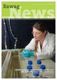
Fig. 1: Irradiance measured by satellites since 1978 (A) [1] compared to sunspot counts (B) in the same period [4].<br />
0.1%<br />
gists. Its value is about 1366 W/m2 . It refers<br />
to the intensity of the sun’s radiation (= irradiance)<br />
at the outer limit of the atmosphere,<br />
at a distance from the sun of 1 astronomical<br />
unit (the average distance of the earth<br />
from the sun). Direct measurements of the<br />
irradiance via satellite have been possible<br />
only since 1978. Since then, it has become<br />
evident that the solar constant is far from<br />
being a constant. In actual fact, it exhibits<br />
cyclical fluctuations with an average period<br />
of 11 years (Fig. 1A) and an average amplitude<br />
of 0.1% [1]. This is a clear indication<br />
that the engine of our climate system is<br />
not constant in its energy output. These<br />
changes in the irradiance are connected<br />
with variations in solar activity. So what was<br />
the situation like prior to 1978, before direct<br />
measurements were possible? EAWAG has<br />
joined a number of international research<br />
groups in an attempt to answer the riddle of<br />
the history of solar activity, as far back in<br />
time as possible [2, 3].<br />
Sunspots as an Indicator<br />
of Solar Activity<br />
Astronomers first collected evidence of variations<br />
in solar activity as much as 400 years<br />
ago. Since the invention of the telescope,<br />
people have observed changes on the sun’s<br />
surface and recorded them by the only<br />
means available – in handmade drawings<br />
[4]. It was soon realized that the number<br />
of dark sunspots varied between 0 and<br />
approximately 300 spots. Just like irradiance,<br />
the number of sunspots fluctuates<br />
in a cycle with a period of around 11 years<br />
(Fig. 1B + 2). The sunspots are an expression<br />
of magnetic processes and therefore a<br />
direct measure of solar activity. The more<br />
active the sun is, the more sunspots there<br />
are on the sun’s surface. They appear dark<br />
since they have a relatively cool surface<br />
temperature of circa 4000 Kelvin (about<br />
3700 °C), and, as a result, emit less energy<br />
locally than the normal surface areas at<br />
circa 5800 Kelvin (about 5500 °C). However,<br />
since the regions immediately surrounding<br />
the spots are hotter than the average, the<br />
EAWAG news 58 8
emission of radiation from a sun with many<br />
sunspots is on the whole greater.<br />
This strict correlation between sunspot<br />
prevalence and irradiance measured by<br />
satellite can be seen clearly in Figure 1A + B,<br />
in which the two curves run parallel to each<br />
other. This has allowed scientists to use the<br />
number of sunspots as the basis for determining<br />
the irradiance arriving at the top of<br />
the earth’s atmosphere, and thereby map<br />
changes in climatic events over the past<br />
400 years.<br />
400 Years of Strongly<br />
Fluctuating Solar Activity<br />
If we look at the four hundred year-long<br />
sunspot record [4], they show that solar<br />
activity has fluctuated significantly more<br />
strongly and more irregularly than satellites<br />
have so far measured (Fig. 2). Practically no<br />
sunspots were recorded during the Maunder<br />
Minimum of 1645–1715, and only a few<br />
during the Dalton Minimum of 1795–1830,<br />
suggesting that the sun was relatively<br />
inactive during both periods. Since then<br />
there has been a steady increase in the<br />
number of sunspots. Lean and fellow researchers<br />
wanted more detailed informa-<br />
Sunspots<br />
200<br />
150<br />
100<br />
50<br />
0<br />
1600<br />
Fig. 2: The sunspot count since 1610 [4], given as an annual average. The more<br />
active the sun, the more sunspots appear on its surface. Along with the clear<br />
11-year cycle an increasing activity since the beginning of the 18 th century can be<br />
observed.<br />
9 EAWAG news 58<br />
Maunder Minimum<br />
Dalton Minimum<br />
1650 1700 1750 1800 1850 1900 1950 2000<br />
Year<br />
tion, and attempted to quantify the intensity<br />
of past solar radiation from the number of<br />
sunspots, concluding that irradiance has<br />
increased by 0.24% since the Maunder<br />
Minimum [2] (Fig. 3). This change is significantly<br />
outside the range of fluctuations<br />
measured to date. From observations of<br />
other solar systems, we know that stellar<br />
radiation can vary greatly – by much as<br />
1% for stars showing similar characteristics<br />
to our sun. In addition, various climatic<br />
traces on the earth indicate that such fluctuations<br />
in the irradiance are not unrealistic.<br />
For example, the occurence of the so-called<br />
Little Ice Age from about 1400 to 1850 coincident<br />
with a period of reduced solar activity.<br />
During this period, large-scale glaciers<br />
advances occured in the Alps that resulted<br />
in large moraine deposits. Furthermore,<br />
from historical sources it is known that the<br />
River Thames froze over in winter during the<br />
Little Ice Age. The ice was particularly thick<br />
in the winter of 1683/84, neatly in the middle<br />
of the Maunder Minimum! Since the winter<br />
of 1813/14, the Thames has stopped freezing<br />
over, and the glaciers have been under<br />
continuous retreat, while the number of sunspots<br />
has been increasing continuously.<br />
11,500 Years of the Sun’s<br />
Activity Recorded in the Polar<br />
Ice Cap<br />
How can we extend the historical research<br />
beyond 400 years into the past? EAWAG<br />
is currently engaged in a project with the<br />
ambitious aim of reconstructing solar activity<br />
over the entire Holocene epoch, which<br />
corresponds to the recent warm period<br />
stretching back about 11,500 years. Once<br />
again, we are dependent on indirect clues.<br />
To measure past solar activity, we are inves-<br />
Solar irradiance (W/m 2 )<br />
1369<br />
1368<br />
1367<br />
1366<br />
1365<br />
1364<br />
1600<br />
Maunder Minimum<br />
tigating the quantity of the cosmogenic<br />
radionuclide beryllium-10 ( 10Be) that was<br />
formed in the past by cosmic radiation, and<br />
which can now be found in frozen precipitation<br />
in the polar ice caps (see lead article<br />
p. 4). Thanks to this thick ice record we can<br />
go very far back in time through relatively<br />
short vertical drill-cores, since the single<br />
annual deposits have been compressed into<br />
thin layers by the pressure of the subsequent<br />
ice layers and by the ice flow. The<br />
GRIP ice core from Greenland examined by<br />
EAWAG is about 3 km long and represents<br />
several hundreds of thousands of years. In<br />
a Sisyphean undertaking, the 10Be concentration<br />
is determined painstakingly layer by<br />
layer (see article from S. Bollhalder and<br />
I. Brunner, p. 6). The 10Be concentration will<br />
enable us to determine the solar activity,<br />
provided two important points are taken into<br />
consideration:<br />
The 10 Be production does not depend on<br />
the solar activity alone, but also on fluctuations<br />
in the earth’s magnetic field. To reconstruct<br />
the solar activity, the influence of the<br />
magnetic field must also be determined.<br />
The 10 Be concentration measurable in the<br />
ice is affected not only by the 10Be produced<br />
in the atmosphere, but also by the amount<br />
of precipitation – the greater the precipitation,<br />
the more the 10Be is diluted. The measure<br />
of solar activity is therefore not simply<br />
the 10Be concentration, but rather the 10Be flux, which gives us the number of 10Be atoms deposited per square meter and<br />
second in the ice.<br />
Our investigations show that the 10Be flux,<br />
and consequently the solar activity, was<br />
very irregular over the entire Holocene<br />
epoch (Fig. 4, blue curve). A low 10Be flux<br />
indicates an active sun and a high 10Be flux<br />
1650 1700 1750 1800 1850 1900 1950 2000<br />
Year<br />
Fig. 3: Irradiance reconstructed back to 1610. The reconstruction is based on<br />
sunspot drawings and observations of stars similar to the sun. Accordingly, irradiance<br />
has increased by 0.24% since the Maunder Minimum.<br />
Adapted from [2].<br />
Dalton Minimum
a less active sun. We are currently working<br />
on expressing this relatively imprecise information<br />
on solar activity as irradiance values.<br />
In parallel to the reconstruction of the irradiance<br />
from the sunspots described previously,<br />
we are attempting to derive the irradiance<br />
from the 10Be data.<br />
Further Climate Clues from<br />
Drifting Icebergs<br />
Further clues indicating the fluctuating influence<br />
of the sun during the Holocene<br />
come from other paleoclimate archives [3].<br />
A number of sediment cores from deep-sea<br />
boreholes in the eastern North Atlantic, at<br />
about the latitude of Ireland, and in the<br />
western Atlantic, at about the latitude of<br />
Newfoundland, have revealed several pronounced<br />
deposits of coarse-grained material.<br />
Whereas normally only fine-grained<br />
clays and muds are deposited in deep-sea<br />
sediments so far from the coast, these<br />
deposits have grain sizes equivalent to, or<br />
even larger than, those of the sand fraction.<br />
Changes in the proportion of IRD [‰]<br />
6<br />
4<br />
2<br />
0<br />
–2<br />
–4<br />
–6<br />
0<br />
10Be flux<br />
IRD<br />
Where does this material come from? A very<br />
probable explanation is that they were<br />
transported there by icebergs. When an<br />
iceberg breaks away from a glacier into the<br />
water (calving), rock debris eroded by the<br />
glacier and frozen to its underside is carried<br />
to sea. When the iceberg melts, this debris<br />
sinks to the seabed. Based on its mode of<br />
transportation, this coarse particulate matter<br />
in the sediment is known as “ice-rafted<br />
debris” (= IRD).<br />
Red Greenland Stone in<br />
Deep-Sea Sediment<br />
Careful examination of the composition of<br />
IRD in the sediment cores reveals clues to<br />
the origin of the particles. Volcanic glass<br />
points to an origin in the volcanic island of<br />
Iceland. Other minerals acting as petrological<br />
tracers could only have originated in<br />
Greenland and Newfoundland. For example,<br />
a red coloring reveals the presence of a mineral<br />
from the “red beds”, a typical rock formation<br />
of eastern Greenland.<br />
The locations of these polar rock fragments<br />
reveal that icebergs have been able to travel<br />
far to the south during the Holocene. This<br />
was possible only when the melting of the<br />
icebergs was delayed by very low air and<br />
seawater temperatures. Therefore, such<br />
large-grain rock deposits are clear<br />
indicators for colder climatic periods. In an<br />
international joint research project, the proportion<br />
of the IRD in a number of sediment<br />
cores was determined (Fig. 4, white curve)<br />
[3] and the results were compared with the<br />
10Be data (Fig. 4, blue curve). Both curves<br />
Fig. 4: Changes in the 10 Be flux in the GRIP ice core (blue curve) and changes in the IRD proportion in the sediment<br />
(white curve). Simplified from [3].<br />
0.06<br />
0.04<br />
0.02<br />
0.00<br />
–0.02<br />
2000 4000 6000 8000<br />
–0.04<br />
10000<br />
Years before today<br />
Changes in the flux of 10 Be (10 6 atoms per cm 2 and year)<br />
high Solar acitivty low<br />
show a quite closely matching pattern. A<br />
higher IRD fraction in the sediment indicates<br />
a cold period, in which icebergs could travel<br />
farther south. During warmer periods, the<br />
icebergs melted much further to the north,<br />
resulting in a lower proportion of IRD in the<br />
sediment samples investigated.<br />
From our results we can derive the following<br />
two correlations:<br />
A “high proportion of IRD cold period”<br />
is associated with a “high 10Be flux inactive<br />
sun”.<br />
A “low proportion of IRD warm period”<br />
is associated with a “low 10Be flux active<br />
sun”.<br />
This means that the drift behavior of the<br />
icebergs in the Holocene appears to have<br />
been controlled by the sun.<br />
All these observations reveal the important<br />
role the sun plays in our climatic system.<br />
Many questions still remain unanswered:<br />
How does our climate system react to<br />
changes in the irradiance? What are the<br />
processes responsible? Do small changes<br />
in solar activity become amplified in the<br />
earth’s internal climate system, e.g. in the<br />
atmosphere? Current research is attempting<br />
to answer these questions, and the search<br />
is on for further clues.<br />
Maura Vonmoos, earth scientist,<br />
reconstructed Holocene solar<br />
activity as part of her doctorate<br />
in the department “Surface<br />
Water”.<br />
[1] Fröhlich C. (2000): Observations of irradiance variations.<br />
Space Science Reviews 94, 15–24.<br />
[2] Lean J., Beer J., Bradley R. (1995): Reconstruction of<br />
solar irradiance since 1610: implications for climate<br />
change. Geophysical Research Letters 22, 3195–3198.<br />
[3] Bond G., Kromer B., Beer J., Muscheler R., Evans M.N.,<br />
Showers W., Hoffmann S., Lotti-Bond R., Hajdas I.,<br />
Bonani G. (2001): Persistent Solar Influence on North<br />
Atlantic Climate During the Holocene. Science 294,<br />
2130 –2136.<br />
[4] Hoyt D.V., Schatten K.H. (1998): Group sunspot numbers:<br />
a new solar activity reconstruction. Solar Physics<br />
179, 189–219.<br />
EAWAG news 58 10
Why Did a Cold Period Follow on<br />
the Heels of the Last Ice Age?<br />
Large-scale climate changes in the northern Atlantic region were<br />
often associated with changes in ocean currents. That is also the<br />
case for the last cold phase of the Würm Ice Age, known as the<br />
Younger Dryas. At this time, a new cold period occurred and the<br />
northern Atlantic region relapsed from a moderate climate back<br />
to glacial conditions in the course of just a few decades. Climate<br />
indicators provide nevertheless contradictory information concerning<br />
the origins of this cold phase. EAWAG is on the trail of additional<br />
clues in an ice core from Greenland.<br />
The Würm Ice Age is the most recent ice<br />
age in the course of earth’s history. It lasted<br />
approximately 100,000 years and ended<br />
only about 10,000 years ago. This ice age<br />
was characterized by rapid climate changes<br />
in the North Atlantic region. The last cold<br />
phase of the Würm Ice Age is known as<br />
the Younger Dryas. It started very suddenly<br />
about 12,700 years ago and lasted circa<br />
1200 years. In this period the mean annual<br />
temperature in Greenland fell by an amount<br />
on the order of 10 °C (Fig. 1A) [1]. A common<br />
hypothesis is that this climate change was<br />
caused by changes in the ocean currents. If<br />
the transport of warm water from the south<br />
to the north is interrupted, this would result<br />
in a sudden temperature fall in the northern<br />
regions. This hypothesis is supported by<br />
a number of observations. However, the<br />
The Radiocarbon Dating Method<br />
11 EAWAG news 58<br />
reconstruction of the atmospheric 14C provides<br />
contradictory evidence. EAWAG wanted<br />
to know more and pursued this contradiction.<br />
Contradictory Evidence<br />
The radioactive carbon isotope 14C (see<br />
box) is a natural trace element of enormous<br />
importance for climate research. It is produced<br />
continuously in the atmosphere by<br />
the action of cosmic radiation, and, after<br />
oxidation to 14CO2, takes part in the global<br />
carbon cycle.<br />
Oceans continuously exchange air and CO2, including radioactive 14C, with the atmosphere.<br />
Within the oceans the distribution<br />
of 14C is governed by oceanic ventilation:<br />
the better the oceans mix globally, the more<br />
14C is transported down to the deeper water<br />
Along with the two stable carbon isotopes, 12C and 13C, there is the radioactive isotope 14C. It<br />
has a half-life of 5730 years; i.e. after 5730 years half of the original 14C in any sample has decayed.<br />
This convenient fact is exploited in the 14C dating method. All living organisms continuously<br />
exchange 14C with their environment. This exchange stops when the organism dies. In the<br />
course of time, the radioactive 14C decays in the organism and the 14C concentration decreases<br />
continuously. By measuring the 14C concentration in a sample, it is therefore possible to estimate<br />
the age, or more precisely expressed, the point in time when the 14C exchange with the<br />
environment was interrupted.<br />
This is, however, only possible precisely when the history of the atmospheric 14C concentration<br />
is known. The reason is simple: if in the past the 14C concentration was higher, then it would<br />
have taken correspondingly longer for the decay to reduce 14C to a specific concentration. Without<br />
knowing the original 14C concentration in the air, one would draw the conclusion that the<br />
sample is younger than it actually is, or over-estimate its age in the opposite case.<br />
For this reason, scientists are developing a 14C calibration curve, which for the past 11,500 years<br />
was accurately dated within ±1 year [2]. This research involves above all fossil tree remains and<br />
sediments with known ages. The measurement of the 14C concentrations in individual tree rings<br />
and sediment layers can then be used to infer the past changes in the atmospheric 14C concentration.<br />
layers, and the more 14C poor water is transported<br />
from the deep sea to the surface.<br />
This process has the consequence that<br />
when ocean mixing is stronger the proportion<br />
of 14C in the atmosphere sinks. If we<br />
assume that the oceanic mixing in the North<br />
Atlantic during the Younger Dryas was in<br />
fact reduced, one would expect to see for<br />
this period, along with the above-described<br />
temperature fall, an accompanying increase<br />
in atmospheric 14C. By measuring the 14C concentration in sediments,<br />
it was possible to reconstruct the<br />
14C concentration in the atmosphere during<br />
the Younger Dryas [3]. As expected, the 14C concentration increased at the beginning<br />
of the Younger Dryas, which confirms the<br />
hypothesis of a reduced oceanic mixing.<br />
However, the 14C atmospheric concentration<br />
fell again long before it became significantly<br />
warmer in the North Atlantic (Fig. 1B).<br />
This contradicts the predicted association<br />
between heat transfer, deepwater formation<br />
and 14C content of the atmosphere. We<br />
wondered therefore what other factors<br />
could have played a role.<br />
Nuclide Production Effect<br />
on the 14C Concentration<br />
The 14C concentration in the atmosphere is<br />
not only determined by oceanic circulation,<br />
but is also influenced by the rate of production.<br />
During a period of weak solar activity,<br />
more 14C is produced in the atmosphere,<br />
which results in an increase in the atmospheric<br />
14C concentration. Such an increase<br />
in 14C occurred, for example, during the<br />
Maunder Minimum between 1645–1715 [4].
At that time the climate in Europe was significantly<br />
colder than today. From astronomical<br />
observations with the recently invented<br />
telescope, it was observed that the sun had<br />
A<br />
δ 18 O<br />
(‰)<br />
B<br />
Δ 14 C<br />
(‰)<br />
C<br />
10Be flux<br />
(103 atoms per cm2 and year)<br />
–32<br />
–34<br />
–36<br />
–38<br />
–40<br />
–42<br />
60<br />
40<br />
20<br />
0<br />
–20<br />
–40<br />
500<br />
450<br />
400<br />
350<br />
300<br />
250<br />
200<br />
Younger Dryas<br />
hardly any sunspots on its surface in this<br />
period (Fig. 2; see also the article by M.<br />
Vonmoos, p. 8). The absence of sunspots<br />
shows that the sun at this time was a lot less<br />
150<br />
14 000 13 000 12 000 11 000 10 000<br />
Age (years before present)<br />
Fig. 1: Temperature, atmospheric 14 C concentration and 10 Be flux during the Younger Dryas.<br />
A) δ 18 O as a measure of the temperature in Greenland (see also lead article).<br />
B) Reconstruction of the atmospheric 14 C concentration expressed as Δ 14 C based on the sediment investigations<br />
in the Cariaco Basin off the north coast of Venezuela. Δ 14 C shows the variation in atmospheric 14 C concentration<br />
with respect to a standard (unit: per mil).<br />
C) 10 Be flux indicating the past radionuclide production.<br />
active than it is today. In the case of the<br />
Maunder Minimum, the observations of sunspots<br />
allowed us to draw a clear association<br />
between the increase in 14C and solar activity.<br />
However, we need another source of<br />
information if we want to infer possible<br />
causes for changes in atmospheric 14C concentration<br />
which occurred further in the<br />
past.<br />
10Be as a Measure of<br />
Atmospheric Radionuclide<br />
Production<br />
An additional and exceedingly interesting<br />
source of information is available through<br />
measurements of the radioactive isotope<br />
Beryllium-10 ( 10Be). Like 14C, 10Be is produced<br />
by the effect of cosmic radiation on<br />
atmospheric atoms (see lead article p. 3).<br />
However, thereafter its terrestrial cycle takes<br />
an entirely different form to that of carbon:<br />
10Be is deposited relatively directly onto the<br />
earth by being washed out of the atmosphere,<br />
and does not, as is the case for 14C, enter a biogeochemical cycle. The history<br />
of the 10Be production rate can be reconstructed<br />
thanks to paleo records. Particularly<br />
successful have been measurements<br />
Number of sunspots<br />
Δ 14 C (‰)<br />
200<br />
150<br />
100<br />
50<br />
0<br />
–30<br />
–20<br />
–10<br />
0<br />
10<br />
Maunder Minimum<br />
Dalton Minimum<br />
20<br />
1600 1650 1700 1750 1800 1850 1900 1950 2000<br />
Year<br />
Fig. 2: Comparison of the number of sunspot groups<br />
with the changes in atmospheric 14 C concentration.<br />
In phases of reduced solar activity, such as during<br />
the Maunder and Dalton Minima, the atmospheric<br />
14 C concentration increased (Δ 14 C is shown inverted).<br />
EAWAG news 58 12
of 10Be in ice cores from central Greenland,<br />
in which 10Be has been deposited from the<br />
atmosphere by precipitation, year by year<br />
and ice layer by ice layer.<br />
If the 14C concentration is dependent only<br />
on one variable, ocean mixing, then we<br />
should find constant deposition of 10Be in<br />
the Younger Dryas ice. If, however, also<br />
changes in the nuclide production rate are<br />
involved during the Younger Dryas, we<br />
should expect a variable 10Be concentration<br />
in the respective ice layers similar to the<br />
variations observed for 14C. Variable Production of<br />
10Be Isotopes<br />
It has in fact been possible to show through<br />
the analysis of 10Be data [5] that the radionuclide<br />
production rate, and, therefore,<br />
most probably also the solar activity during<br />
the Younger Dryas, was indeed variable<br />
(Fig. 1C). If one converts the 10Be data to 14C values, it appears that a large part of the<br />
atmospheric 14C variation can be explained<br />
by this variable rate of production (Fig. 3A).<br />
However, the 14C variations observed during<br />
the Younger Dryas can only be explained<br />
satisfactorily by including in addition the<br />
A<br />
Δ 14 C<br />
(‰)<br />
B<br />
Δ 14 C<br />
(‰)<br />
60<br />
40<br />
20<br />
13 EAWAG news 58<br />
0<br />
–20<br />
–40<br />
–60<br />
60<br />
40<br />
20<br />
0<br />
–20<br />
–40<br />
Younger Dryas<br />
effects of a 30% reduction in ocean circulation<br />
(Fig. 3B) [6]. Our analyses confirm,<br />
therefore, that the Younger Dryas is in fact<br />
associated with a reduced deepwater formation.<br />
The trigger for this abrupt climate<br />
change is still unclear. It is apparent, though,<br />
that the radionuclide production at the start<br />
of the cold phase was higher. This clue suggests<br />
that a reduced solar activity could<br />
have been the cause for the onset of the<br />
cold spell.<br />
With the example of the Younger Dryas, we<br />
have been able for the first time by comparison<br />
of 10Be and 14C data to distinguish<br />
between changes in the production rates<br />
–60<br />
14,000 13,000 12,000<br />
Age (years before present)<br />
12,000 10,000<br />
Fig. 3: Model of the atmospheric 14 C concentration (light-blue curves):<br />
A) taking only into account radionuclide production,<br />
B) taking into account both radionuclide production and ocean circulation.<br />
For comparison the actual reconstructed 14 C concentration is again represented (dark-blue curve from Fig. 1B).<br />
and changes in the carbon cycle. This<br />
process is usable for the whole time period<br />
covered by the 14C method (i.e. the last<br />
50,000 years), and will play an important<br />
role in future investigations concerning the<br />
global changes in the carbon cycle.<br />
Raimund Muscheler worked<br />
on this project as part of his<br />
doctorate in the “Surface<br />
Waters” department. Since<br />
2003 he has been working as<br />
a post-doctorate fellow at the<br />
University of Lund in Sweden.<br />
[1] Johnsen S.J., Clausen H.B., Dansgaard W., Fuhrer K.,<br />
Gundestrup N., Hammer C.U., Iversen P., Jouzel J.,<br />
Stauffer B., Steffensen J.P. (1992): Irregular glacial<br />
interstadials recorded in a new Greenland ice core.<br />
Nature 359, 311–313.<br />
[2] Stuiver M., Reimer P.J., Bard E., Beck J.W., Burr G.S.,<br />
Hughen K.A., Kromer B., McCormac G., Van der<br />
Pflicht J., Spurk M. (1998): INTCAL98 radiocarbon<br />
age calibration, 24,000 –0 cal BP. Radiocarbon 40,<br />
1041–1083.<br />
[3] Hughen K., Overpeck J.T., Lehmann S., Kashgarian<br />
M., Southon J., Peterson L.C., Alley R., Sigman D.M.<br />
(1998): Deglacial changes in ocean circulation from an<br />
extended radiocarbon calibration. Nature 391, 65–68.<br />
[4] Eddy J.A. (1976): The Maunder Minimum. Science<br />
192, 1189–1201.<br />
[5] Finkel R.C., Nishiizumi K. (1997): Beryllium 10 concentrations<br />
in the Greenland ice sheet project 2 ice core<br />
from 3–40 ka. Journal of Geophysical Research 102,<br />
26 699–26 706.<br />
[6] Muscheler R., Beer J., Wagner G., Finkel R.C. (2000):<br />
Changes in deep-water formation during the Younger<br />
Dryas cold period inferred from a comparison of 10Be and 14C records. Nature 408, 567–570.
The Compass in the Ice<br />
Everyone knows that a freely-moving magnetic needle will align<br />
itself to north, making it rather useful for finding one’s way in<br />
unknown areas or when visibility is poor. The principle of the<br />
magnetic compass has been known for more than a thousand<br />
years, and has been of inestimable value to navigators. Even<br />
migratory birds and other animals seem to have an inbuilt compass<br />
which permits them to home in on their destinations with<br />
uncanny precision. However, a compass several thousand years<br />
ago would not have pointed to the north pole; throughout the<br />
earth’s history, the geomagnetic field has reversed its polarity<br />
again and again.<br />
Even though the earth’s magnetic field, or<br />
geomagnetic field (Fig. 1) has been investigated<br />
in detail for more than 300 years,<br />
Einstein referred to it as one of the greatest<br />
unsolved mysteries of science. Since then<br />
many outstanding questions regarding the<br />
origin and alignment of the geomagnetic<br />
field (Fig. 2) have been answered (see box).<br />
However, the reason why the polarity of the<br />
magnetic field has reversed itself on a number<br />
of occasions throughout earth’s history<br />
is still a riddle (Fig. 3). Before an answer to<br />
this riddle can be found, the polarity and<br />
strength of the magnetic field must be reconstructed<br />
as far back in time as possible.<br />
EAWAG has been able to show that the<br />
measurement of radioisotopes in ice cores<br />
represents a new method of calculating the<br />
geomagnetic field.<br />
Paleo Records Reveal the<br />
Earth’s Magnetic Field<br />
Traditionally, paleomagnetists use sediments<br />
and volcanic rock to reconstruct the<br />
geomagnetic field. In sediments, it is the<br />
magnetic particles which have been deposited<br />
layer by layer throughout the past<br />
that are of interest. As long as these particles<br />
remained mobile within the sediment,<br />
they would align themselves with the<br />
magnetic field like a compass needle. The<br />
stronger the magnetic field, the more they<br />
display this characteristic. This allows the<br />
direction and intensity of the earth’s past<br />
magnetic field to be determined from sediment<br />
cores. Similarly, volcanic rock reveals<br />
the past through the outpouring of high temperature<br />
rock mass from deep within the<br />
earth’s interior during a volcanic eruption.<br />
Origin, Orientation and Strength of the Geomagnetic Field<br />
The earth is surrounded by a magnetic field (Fig. 1). The origin of this magnetic field lies in the<br />
convection fluxes of fluid iron in the earth’s center: as in the case of water, hot iron rises to the<br />
outside and cold iron sinks to the center.<br />
The direction of the axis of the magnetic field does not correspond to the earth’s axis; i.e. the<br />
magnetic poles do not coincide with the geographic poles (Fig. 1). In addition, the magnetic<br />
poles are continually migrating. In the last 2000 years, the magnetic north pole has shifted thousands<br />
of kilometers over the Arctic (Fig. 2). About 300 years ago it reached Greenland. Today it<br />
lies in Canada, and it is unclear where it will go in the future.<br />
Not only has the orientation of the magnetic field varied over time, its strength has done likewise.<br />
Of particular interest is when the field strength approaches zero. In this case, when the<br />
field intensity increases again, a reversal of polarity can occur, meaning that the magnetic north<br />
pole is suddenly in the southern hemisphere, where it usually remains for several hundred thousand<br />
years before flipping back again to the northern hemisphere. The timing of a reversal does<br />
not appear to follow any particular pattern, and is, therefore, impossible to foresee. The last<br />
reversal of polarity, the so-called Brunhes-Matuyama polarity reversal, occurred some 780,000<br />
years ago (Fig. 3).<br />
So long as the lava is fluid, it is not magnetizable.<br />
Only during cooling do ferro-magnetic<br />
particles align themselves with the<br />
geomagnetic field.<br />
These methods of geomagnetic field reconstruction<br />
are most applicable when the<br />
magnetic field was strong, the sediment<br />
homogeneous and rich in magnetic particles,<br />
and the recorded magnetic field not<br />
disturbed subsequently by other processes.<br />
axis of the earth<br />
Fig. 1: The geomagnetic field can be depicted in simplified<br />
form as a dipole field produced by an imaginary<br />
bar magnet located at the earth’s center. This bar<br />
magnet is slightly askew with respect to the earth’s<br />
axis of rotation.<br />
90°<br />
1 AD<br />
180° 0°<br />
270°<br />
1990 AD<br />
1690 AD<br />
Fig. 2: Migration of the magnetic north pole through<br />
the Arctic during the last 2000 years [1]. The migration<br />
continues.<br />
EAWAG news 58 14
15 EAWAG news 58<br />
Brunhes<br />
normal polarity<br />
Matuyama<br />
reversed polarity<br />
Gauss<br />
normal polarity<br />
Gilbert<br />
reversed polarity<br />
Age<br />
(millions of years)<br />
Fig. 3: Reversals of the polarity of the geomagnetic<br />
field over the past 4 million years. In the light-blue<br />
time periods the polarity was the same as today; in<br />
the dark-blue periods the polarity was reversed. Some<br />
epochs are named after researchers dedicated to<br />
solving the riddles of the geomagnetic field.<br />
Geomagnetic field intensity<br />
1.5<br />
1.0<br />
0.5<br />
1<br />
2<br />
3<br />
4<br />
The Radioisotope Method<br />
The new radioisotope method is based on<br />
the analysis of polar ice cores. Although<br />
this ice consists almost entirely of only the<br />
purest of water, and contains effectively<br />
no magnetic particles, it can nevertheless<br />
reveal invaluable information concerning<br />
the history of the geomagnetic field. This<br />
information can be read from the trace<br />
amounts of radioisotopes, such as beryllium-10<br />
( 10Be) and chlorine-36 ( 36Cl), found in<br />
the ice. A strong geomagnetic field shields<br />
the earth from cosmic radiation, reducing<br />
the production of radionuclides. When the<br />
magnetic shield is “switched off”, however,<br />
the global nuclide production rate more than<br />
doubles. If we assume that the slow change<br />
in 10Be and 36Cl found in the ice is caused<br />
by the magnetic field, and that the faster<br />
solar variations are averaged out, then we<br />
have at our disposal a new, completely<br />
different method of reconstructing the historical<br />
strength of the geomagnetic field. It<br />
differs from the traditional methods in that<br />
its sensitivity actually increases with de-<br />
reconstructed from 10 Be and 36 Cl data from the GRIP ice core<br />
reconstructed from sediment core data from the Mediterranean Sea<br />
0<br />
20,000 30,000 40,000<br />
Years before present<br />
50,000 60,000<br />
Fig. 4: Reconstruction of the geomagnetic field strength over the time period 20,000 –60,000 years before present.<br />
Comparison of the radioisotope method (dark-blue curve: combined 10 Be and 36 Cl data from the GRIP ice core [2])<br />
with traditional methods (light-blue curve: orientation of magnetic particles in a sediment core from the Mediterranean<br />
Sea [3]). The gray band represents the range of uncertainty of the radioisotope method. The range of uncertainty<br />
of the traditional method is not shown.<br />
creasing field strength. Another advantage<br />
of this new method is that it is hardly affected<br />
at all by local variations in the magnetic<br />
field.<br />
Is the Radioisotope Method<br />
Reliable?<br />
In order to assess whether the radioisotope<br />
method does in fact produce reliable results,<br />
we have made a direct comparison of<br />
the two methods. Figure 4 shows the magnetic<br />
field strengths as reconstructed from<br />
10 Be and 36 Cl concentrations in the GRIP<br />
ice core from Greenland [2], and from traditional<br />
measurements of Mediterranean Sea<br />
sediment cores [3]. Apart from a few digressions,<br />
the results of the two methods agree<br />
well. The radionuclide measurements, for<br />
example, confirm that the earth’s magnetic<br />
field weakened about 40,000 years ago to<br />
around 10% of its current strength. However,<br />
just before a reversal of polarity could<br />
occur, it returned to its old state.<br />
The radioisotope method has therefore<br />
passed its baptism of fire. In the future, it<br />
can be used to analyze the entire time range<br />
covered by ice cores and sediment cores,<br />
thereby making it possible to reconstruct<br />
the geomagnetic field back to about one<br />
million years ago.<br />
And what about the future? When can we<br />
expect a new reversal of polarity? For about<br />
2000 years the magnetic field strength has<br />
decreased continuously, so if the rate remains<br />
constant we will experience another<br />
magnetic polarity reversal within about another<br />
2000 years. We humans will not notice<br />
this, but for migratory birds, which rely on<br />
the geomagnetic field for orientation, it is<br />
unclear what effect this will have on their<br />
ability to find their destinations.<br />
Jürg Beer, portrait on page 5.<br />
[1] Hongre L., Hulot G., Khokhlov A. (1998): An analysis<br />
of the geomagnetic field over the past 2000 years.<br />
Physics of the Earth and Planetary Interiors 106,<br />
311–335.<br />
[2] Wagner G., Masarik J., Beer J., Baumgartner S.,<br />
Imboden D., Kubik P.W., Synal H.-A., Suter M. (2000):<br />
Reconstruction of the geomagnetic field between 20<br />
and 60 kyr BP from cosmogenic radionuclides in the<br />
GRIP ice core. Nuclear Instruments and Methods in<br />
Physics Research B 172, 597–604.<br />
[3] Tric E., Valet J.P., Tucholka P., Paterne M., LaBeyrie L.,<br />
Guichard F., Tauxe L., Fontugne M. (1992): Paleointensity<br />
of the geomagnetic field during the last<br />
80,000 years. Journal of Geophysical Research 97,<br />
9337–9351.
Cosmic Radiation<br />
and Clouds<br />
Ice cores provide abundant information about past climate changes.<br />
They can also provide answers to very specific questions and<br />
the means of testing hypotheses. One such hypothesis proposes<br />
that climate changes are caused primarily by changes in the intensity<br />
of cosmic radiation. If this is correct, it relegates the enhanced<br />
greenhouse effect to a secondary role – a politically explosive<br />
hypothesis which demands closer analysis.<br />
In 1997, Danish scientists came before the<br />
press and announced, not without some<br />
pride, that they had found the explanation<br />
for the global climate warming that has occurred<br />
over the past 150 years [1]. According<br />
to them, the decisive role was played<br />
neither by the greenhouse effect nor by the<br />
solar constant (see lead article on p. 3), but<br />
rather by global cloud cover (see box). Their<br />
work suggested that cloud formation is<br />
affected by cosmic radiation, which underwent<br />
a significant decrease during the 20th century. This work found wide public appeal.<br />
Newspaper, magazine, and television<br />
reports followed the debate blow by blow,<br />
and a book on the subject, “The Manic Sun”<br />
[2], also appeared. Since the Danish hypothesis<br />
presents global climate warming as a<br />
natural process, and therefore exonerates<br />
humans of any responsibility for it, it was<br />
particularly welcome in those circles of<br />
Temperature variation (°C)<br />
0.4<br />
0.2<br />
0.0<br />
–0.2<br />
–0.4<br />
1850<br />
1900 1950 2000<br />
Year<br />
Fig. 1: Comparison of global temperature variations since 1850 (relative to the period<br />
1961–1990) with the concentration of CO 2 in the atmosphere. Temperature curve:<br />
average of innumerable measurements from different weather stations [4].<br />
CO 2 curve: data up to 1953 from analyses of air bubbles in the Siple ice core [5];<br />
since 1958 direct CO 2 measurements at Mauna Loa [6]. ppm = parts per million.<br />
industry and politics which are keen to avoid<br />
the necessity of implementing any measures<br />
to reduce the emission of greenhouse<br />
gases. Here, science was challenged, and<br />
also EAWAG entered into the fray [3]. Once<br />
again climate change demonstrated itself<br />
to be a very complex process which resists<br />
explanation in terms of a single process. The<br />
major potential causes of climate changes<br />
are greenhouse gases, solar irradiance,<br />
aerosols, volcanic eruptions and internal<br />
variations within the climate system. In the<br />
following discussion, we focus on the first<br />
two of these.<br />
Greenhouse Gases and<br />
Solar Radiation<br />
Since about 1850, the temperature in the<br />
northern hemisphere has undergone an<br />
almost continuous increase (Fig. 1) [4–6].<br />
Among the possible causal factors under<br />
400<br />
380<br />
360<br />
340<br />
320<br />
300<br />
280<br />
CO 2 concentration (ppm)<br />
Variations in cloud cover (%)<br />
3<br />
2<br />
1<br />
0<br />
–1<br />
–2<br />
–3<br />
1980<br />
discussion for this climate change are the<br />
increase in the concentrations of greenhouse<br />
gases present in the atmosphere, and<br />
variations in solar activity:<br />
If we look, for example, at the behaviour of<br />
CO2, a major greenhouse gas, an exponential<br />
increase in its concentration has indeed<br />
occurred over the past 150 years. This increase<br />
has been particularly steep since the<br />
middle of the 20th century (Fig. 1). The cause<br />
of the exponential increase is generally acknowledged<br />
to be the increasing consumption<br />
of fossil fuels. Air temperature, on the<br />
other hand, fluctuates greatly. Particularly<br />
noteworthy are two temperature rises from<br />
1910 to 1940 and from 1970 to the present.<br />
Between 1940 and 1970 there was in fact<br />
a slight cooling. These fluctuations do not<br />
correspond to the exponentially growing<br />
CO2 concentration.<br />
As regards solar radiation, satellite measurements<br />
made since 1980 show that the<br />
radiation intensity is not constant, but rather<br />
fluctuates through an 11-year sunspot cycle<br />
(see Fig. 1, p. 8). Looking more closely, however,<br />
it can be seen that the solar constant<br />
of 1366 W/m2 varies by less than 2 W/m2 over a sunspot cycle, which is just 0.15%<br />
– too low to explain the observed temperature<br />
fluctuations.<br />
Clouds<br />
Cosmic radiation<br />
1985 1990 1995<br />
Year<br />
Fig. 2: Cloud cover variations from1980 to 1995, which exceed 2%, follow the variations<br />
in cosmic radiation very well [1]. On the same scale, the 12-month running<br />
mean cloud cover (expressed as a percentage change) is plotted against normalized<br />
monthly mean measurements of cosmic radiation in Colorado (USA).<br />
EAWAG news 58 16
Therefore neither of these two factors alone<br />
can explain the climate warming. So much<br />
for the level of understanding today, with<br />
which the Danes are in agreement. But how<br />
do the Danes argue further?<br />
Influence of Clouds<br />
The Danish scientists wondered whether<br />
the cosmic radiation could have an effect on<br />
our climate. According to their idea (see<br />
box), the more cosmic radiation that reaches<br />
the earth from space, the greater the<br />
global cloud cover should be. To test this<br />
hypothesis, they examined satellite pictures<br />
of the cloud cover from the years 1980 to<br />
1995, and compared them to the intensity of<br />
the cosmic radiation. They found that the<br />
cloud cover in this period varied by about<br />
2% and followed the variation in cosmic<br />
radiation exactly (Fig. 2). Their hypothesis<br />
appears to be fundamentally able to explain<br />
past observed climate fluctuations. Nevertheless,<br />
the work of the Danes stands on<br />
wobbly legs, since their data analysis is limited<br />
to a tiny time window of only 15 years.<br />
To strengthen their hypothesis, it would be<br />
necessary to obtain further data on cosmic<br />
radiation and climate over the past few<br />
hundred or even thousand years. EAWAG<br />
has found such additional information in the<br />
Greenland ice core.<br />
Weak Cosmic Radiation in the<br />
Past 300 Years<br />
If we look back over the past 300 years, we<br />
see that the cosmic radiation has in general<br />
decreased. On the one hand, we know this<br />
from direct measurements of cosmic radiation<br />
by neutron monitors which have been<br />
operating since the 1950s; on the other<br />
hand, we can use radionuclides such as<br />
beryllium-10 ( 10Be) and chlorine-36 ( 36Cl), which are deposited in Greenland, as indirect<br />
parameters for the reconstruction of<br />
the cosmic radiation in the past. The reduction<br />
in cosmic radiation would seem to be<br />
due to increased solar activity (see Figs. 2<br />
and 3, p. 9). According to the Danish hypothesis,<br />
one would expect for this period,<br />
17 EAWAG news 58<br />
David Parker<br />
Fig 3: Cosmic radiation arrives with high energy from outer space and penetrates the atmosphere, where it collides<br />
with the atoms in the air. This produces secondary particles, which in turn collide with other air atoms, splitting<br />
them into cosmogenic radionuclides. At the same time the primary and secondary particles ionize the air, so that –<br />
according to the Danish hypothesis – more clouds are formed. The above illustration is a montage. It shows at<br />
which height in the atmosphere the various processes occur.<br />
The Cloud Hypothesis<br />
The hypothesis of the Danish scientists Svensmark and Friis-Christensen [1] appears simple<br />
and enlightening: cosmic radiation – high-energy particles from deep space – penetrates the<br />
atmosphere and ionizes the air (Fig. 3). Moisture in the air condenses on these ions to form<br />
small water droplets, resulting in cloud formation. The more clouds that are present, the less<br />
solar radiation reaches the earth’s surface, and temperatures fall. As a corollary to this, it gets<br />
warmer if there are fewer clouds in the sky and the sun’s rays can reach the earth’s surface<br />
unhindered.<br />
How much cosmic radiation can reach the earth’s atmosphere depends on the interplay of two<br />
factors: solar activity and the earth’s magnetic field. The sun is continually spewing out glowing<br />
gas into space. This gas expands to form the so-called solar wind, and in the process carries<br />
with it the sun’s magnetic field. The solar magnetic field forms an external protective shield<br />
around the earth, which prevents the cosmic radiation from entering the earth’s atmosphere<br />
(see Fig. 4 on page 5). In addition, the earth’s magnetic field provides an internal protective<br />
shield, reinforcing the external shield. The more active the sun is and the stronger the magnetic<br />
field, the less cosmic radiation enters the earth’s atmosphere.
A<br />
10Be + 36Cl flux<br />
(relative units)<br />
B<br />
δ 18 O (‰)<br />
C<br />
CH 4 concentration (ppb)<br />
2.0<br />
1.8<br />
1.6<br />
1.4<br />
1.2<br />
1.0<br />
–42<br />
–41<br />
–40<br />
–39<br />
–38<br />
350<br />
400<br />
450<br />
500<br />
550<br />
20,000 25,000 30,000 35,000 40,000 45,000 50,000 55,000<br />
Years before present<br />
with its decreasing intensity of cosmic radiation,<br />
a matching decrease in cloud cover,<br />
and thereby climate warming. So far so<br />
good for the cloud hypothesis.<br />
Strong Cosmic Radiation<br />
40,000 years ago<br />
If we go even further into the past, the situation<br />
changes. About 40,000 years ago we<br />
find a period of about 3000 years during<br />
which the cosmic radiation was relatively<br />
strong. During this period the earth suddenly<br />
lost its protective shield, and the cosmic<br />
radiation penetrated the earth’s atmosphere<br />
with a considerably increased intensity. The<br />
cause lay in the earth’s magnetic field,<br />
whose intensity at that time had sunk to<br />
about 10% of today’s value. If the Danish<br />
hypothesis is true, the cloud cover in this<br />
10 Be + 36 Cl<br />
as indicators of cosmic radiation<br />
δ 18 O<br />
as a climate indicator<br />
CH 4<br />
as a climate indicator<br />
60,000<br />
Fig. 4: Comparison of combined 10 Be and 36 Cl data (A) with the two climate parameters δ 18 O (B) and CH 4 (C) in the<br />
GRIP ice core. Resulting from a weakening of the earth’s magnetic field around 40,000 years before present (grey<br />
area), the intensity of the cosmic radiation increased, and more 10 Be and 36 Cl was formed. Contradicting the Danish<br />
theory, neither of the climate parameters shows any indication of a climate cooling. The calculated correlation coefficients<br />
approach zero. ppb = parts per billion.<br />
period should have increased, resulting in a<br />
significant climate cooling [3].<br />
Once again the Greenland ice core provides<br />
ample information to test this hypothesis.<br />
Fig. 4A shows the combined 10Be and 36Cl data. In this figure, a peak around 40,000<br />
years ago springs to the eye. This radionuclide<br />
peak meets our expectations exactly,<br />
since stronger cosmic radiation increases<br />
radionuclide production. At the same time,<br />
two climate parameters, δ18O and methane,<br />
were measured in the ice core. According to<br />
the cloud hypothesis, it should have become<br />
significantly colder, so we would expect<br />
a clear reduction in δ18O and methane<br />
to have occurred during this same period.<br />
This is, however, not the case (Figs. 4B and<br />
C). The two climate parameters δ18O and<br />
methane correspond well with each other,<br />
but do not match the 10Be/ 36Cl curve. Our<br />
results clearly contradict the cloud hypothesis.<br />
Since all the parameters are measured<br />
in the same ice core, this important result<br />
does not depend on how well the ice core is<br />
dated.<br />
Too Ambitious Interpretations<br />
In the meantime, further disagreements<br />
have arisen, in particular with regard to the<br />
analysis of the latest cloud data, which<br />
no longer follow the cosmic radiation data.<br />
At the moment it looks bad for the cloud<br />
hypothesis, although the last word has not<br />
yet been uttered. Once again it has been<br />
made apparent that climate is a complex<br />
beast, and that changes in climate cannot<br />
be explained in terms of a single, simple<br />
mechanism. On the other hand, evidence is<br />
mounting that prior to 1970 the sun played<br />
a very central role, not in terms of cosmic<br />
radiation, but directly, through variations in<br />
the intensity of solar radiation (see article by<br />
M. Vonmoos, p. 8). The strong warming that<br />
has occurred over the past 30 years can<br />
nevertheless not be explained by the sun.<br />
There is every indication that it is the result<br />
of increases in anthropogenic emissions of<br />
greenhouse gases. In a few years we will<br />
know with certainty, but with no possibility<br />
of avoiding the consequences.<br />
Jürg Beer, portrait on p. 5.<br />
[1] Svensmark H., Friis-Christensen E. (1997): Variation of<br />
cosmic ray flux and global cloud coverage – a missing<br />
link in solar-climate relationships. Journal of Atmospheric<br />
and Solar-terrestrial Physics 59, 1225–1232.<br />
[2] Calder N. (1997): Die launische Sonne: Dr. Böttiger<br />
Verlags-GMBH, Wiesbaden.<br />
[3] Wagner G., Livingstone D.M., Masarik J., Muscheler<br />
R., Beer J. (2001): Some results relevant to the discussion<br />
of a possible link between cosmic rays and<br />
the Earth’s climate. Journal Geophysysical Research<br />
106, 3381–3388.<br />
[4] Jones P.D., Parker D.E., Osborn T.J., Briffa K.R.<br />
(2001): Global and hemispheric temperature anomalies<br />
– land and marine instrumental records. In: Trends:<br />
A Compendium of Data on Global Change. Carbon<br />
Dioxide Information Analysis Center, Oak Ridge, USA.<br />
[5] Neftel A., Moor E., Oeschger H., Stauffer B. (1985):<br />
Evidence from polar cores for the increase in atmospheric<br />
CO2 in the past two centuries. Nature 315,<br />
45–47.<br />
[6] Keeling C.D., Whorf T.P. (2003): Atmospheric CO2 concentrations<br />
(ppmv) derived from in situ air samples<br />
collected at Mauna Loa Observatory, Hawaii. Made<br />
available online by C.D. Keeling.<br />
EAWAG news 58 18
Ice Cover on Lakes and Rivers<br />
Climate Trends Inferred from Historical Records<br />
The longer and colder a winter is, the earlier lakes freeze and the<br />
later they thaw. This is obvious intuitively even if we ignore the<br />
underlying meteorological complexities. EAWAG decided to take a<br />
closer look at this phenomenon by analyzing long series of historical<br />
observations of the timing of freeze-up and break-up of<br />
lakes such as the Lej da San Murezzan in Switzerland and Lake<br />
Baikal in Siberia. From these data, conclusions can be drawn<br />
about past and future climate forcing.<br />
Causally, the formation of an ice cover on<br />
lakes and rivers in winter and its disappearance<br />
in the following spring are the end<br />
results of complex series of mixing, freezing<br />
and thawing processes driven ultimately by<br />
many meteorological forcing factors. By far<br />
the most important of these factors is air<br />
temperature, so that the formation or disappearance<br />
of ice on a lake or river can often<br />
be viewed in an empirical sense simply as<br />
a temporally integrated response to the<br />
seasonal variability in air temperature. The<br />
reverse is also true, allowing conclusions<br />
about the air temperatures that prevailed<br />
in the vicinity of a water body at some time<br />
in the past to be drawn from historical observations<br />
of the timing of freeze-up and<br />
break-up. Since air temperature is a very<br />
spatially coherent meteorological variable –<br />
Freeze-up date<br />
January<br />
December<br />
November<br />
19 EAWAG news 58<br />
Lake Baikal<br />
Mendota<br />
Kallavesi<br />
Red River<br />
air temperatures are usually well correlated<br />
over several hundred kilometers – historical<br />
variations in the timing of break-up do not<br />
merely reflect variations in local weather, but<br />
– much more usefully – variations in regional<br />
or even supraregional climate.<br />
Shorter and Thinner Ice Cover –<br />
A Response to Climate Change?<br />
Historical observations of the calendar<br />
dates of freeze-up (defined as the first day<br />
of total ice cover) and break-up (defined as<br />
the first completely ice-free day) of lakes<br />
and rivers in Canada, the USA, Finland,<br />
Switzerland, Russia and Japan provide<br />
consistent evidence that lakes and rivers<br />
around the Northern Hemisphere have been<br />
freezing later and thawing earlier since at<br />
least the middle of the 19th century (Fig. 1)<br />
Fig. 1: Time-series of the calendar dates of freeze-up (left) and break-up (right) for a small but representative selection of lakes and rivers distributed around the northern hemisphere.<br />
Data presented as a 10-year running mean, from [1].<br />
Break-up date<br />
May<br />
Kallavesi<br />
Lej da<br />
S. Murezzan<br />
Tornionjoki<br />
Lake Baikal<br />
Red River<br />
Mendota<br />
1800 1820 1840 1860 1880 1900 1920 1940 1960 1980 2000 1800 1820 1840 1860 1880 1900 1920 1940 1960 1980 2000<br />
Year<br />
Year<br />
June<br />
April<br />
March<br />
[1]. These long-term historical freezing and<br />
thawing trends average around 6 days per<br />
100 years, which corresponds to an air temperature<br />
increase of 1.2 °C per 100 years.<br />
Thus historical cryophenological data from<br />
lakes and rivers lend support to the hypothesis<br />
of past and current global warming, but<br />
2<br />
1 Mendota<br />
2 Red River<br />
1<br />
6<br />
3 Tornionjoki<br />
4 Kallavesi<br />
3 4 5<br />
5 Lake Baikal<br />
6 Lej da<br />
S. Murezzan
Fig. 2: The annual horse race on the frozen Lej da San Murezzan, Switzerland.<br />
also make it clear that global warming will<br />
have a substantial effect on the timing and<br />
duration of ice cover on lakes and rivers<br />
in the future. This is likely to have socioeconomic<br />
and ecological impacts with both<br />
negative and positive aspects. At high latitudes,<br />
for instance, the transport of people<br />
and goods across large lakes (e.g., Lake<br />
Baikal) and wide rivers (e.g., the Yukon River)<br />
in winter will on the one hand be made<br />
more difficult and more costly by a diminution<br />
of the thickness of the ice cover and a<br />
shortening of the ice season. On the other<br />
hand, an increase in the duration of the<br />
Shared variance r 2 (%)<br />
70<br />
60<br />
50<br />
40<br />
30<br />
20<br />
10<br />
Bever (r 2 = 64%)<br />
Neuchâtel<br />
(r 2 = 61%)<br />
0<br />
February March<br />
p = 0.01<br />
April<br />
May<br />
Fig. 3: Proportion of variance shared (r 2 ) between the<br />
timing of break-up of Lej da San Murezzan (Upper<br />
Engadine, Switzerland) and integrated air temperatures<br />
at Bever, 7 km from the lake, and in Neuchâtel,<br />
230 km west of the lake. The air temperatures were<br />
integrated over 51 days. Each curve consists of 120<br />
r 2 values which occur in the middle of each of 120<br />
51-day periods. The shaded area represents the usual<br />
range of break-up date (mean break-up date ± one<br />
standard deviation). The p = 0.01 significance level is<br />
shown as a horizontal dotted line. Adapted from [3].<br />
open-water season will benefit transport by<br />
ships and barges (e.g., on Lake Superior).<br />
Ecologically, a shortening of the ice season<br />
will result in better oxygen conditions in<br />
lakes that are normally under ice for much of<br />
the winter [2], so that the danger of winter<br />
fish-kills due to prolonged anoxia will be<br />
lessened. However, a shift towards earlier<br />
break-up will generally result in a corresponding<br />
shift towards earlier spring turnover,<br />
and hence to an earlier spring phytoplankton<br />
bloom, but at lower light intensities. This<br />
change in environmental conditions at such<br />
an important time of the year is likely to result<br />
in a shift in the species composition of<br />
the phytoplankton community, with potentially<br />
wide-ranging ecological ramifications<br />
for the lake concerned.<br />
Ice Data from the<br />
Lej da San Murezzan<br />
In Switzerland, the longest available series<br />
of ice observations is that of the break-up<br />
date of the Lej da San Murezzan, the “Lake<br />
of St. Moritz”, located at 1768 m a.s.l. in the<br />
mountains of the Upper Engadine (Fig. 2).<br />
This valuable data series, which begins in<br />
1832 and continues without interruption up<br />
to the present (Fig. 1), is unique in central<br />
Europe. Because of its length and because<br />
reliable instrumental air temperature measurements<br />
beginning in the second half of<br />
the 19th century are available from various<br />
meteorological stations in Europe, this series<br />
is particularly suited to investigating the<br />
relationship between break-up date and air<br />
temperature on various spatial scales.<br />
Tourist Office St. Moritz<br />
Supraregional Climate<br />
Influences Ice Cover<br />
The Lej da San Murezzan thaws, on average,<br />
on 12 May. Our analysis (Fig. 3) shows<br />
that the timing of break-up is highly correlated<br />
with the local air temperature, with a<br />
maximum shared variance (r2 ) of 64% [3];<br />
i.e., 64% of the variability in the timing of<br />
break-up can be explained statistically by<br />
the variability of the air temperature. Consequently,<br />
the mean local air temperature over<br />
a time period of 4–8 weeks in spring can be<br />
estimated quite well from the calendar date<br />
of break-up of the lake (Fig. 3). Air temperatures<br />
measured quite far from the lake,<br />
however, also correlate well with the Lej<br />
da San Murezzan break-up dates [3, 4]. For<br />
instance, correlations with the air temperature<br />
at Neuchâtel, about 230 km from the<br />
lake, yield a maximum shared variance of<br />
61%, only slightly lower than the value obtained<br />
from the correlation with the local air<br />
temperature at Bever (Fig. 3). This implies<br />
that the thawing of Lej da San Murezzan –<br />
and, by analogy, of other alpine lakes – is<br />
primarily a response to climatic forcing on a<br />
regional scale rather than to local meteorological<br />
idiosyncrasies.<br />
Extending the analysis even further afield,<br />
statistically significant relationships were<br />
found with air temperatures measured in the<br />
Netherlands and the United Kingdom, but<br />
not with mean Northern Hemisphere air<br />
temperatures, implying that interannual variability<br />
in lake ice break-up is more the result<br />
of climatic forcing on a synoptic scale than<br />
on a global scale. A companion article on<br />
p. 23 of this issue of EAWAG news describes<br />
the relationship between the timing of ice<br />
break-up on Northern Hemisphere lakes<br />
and the large-scale climatic phenomenon<br />
known as the North Atlantic Oscillation<br />
(NAO).<br />
Ice Data from Lake Baikal<br />
The world’s deepest (1650 m) and largest<br />
(23,000 km3 ) freshwater lake is Lake Baikal,<br />
situated in the Baikal Rift Zone of eastern<br />
Siberia (Fig. 4). It is over 600 km long, has a<br />
EAWAG news 58 20
mean breadth of about 50 km, and contains<br />
no less than 20% of all liquid fresh water<br />
on the surface of the planet. The lake is<br />
estimated to be over 25 million years old,<br />
has the highest biodiversity of any lake now<br />
existing, and supports a unique ecological<br />
system with about 1500 floral and more than<br />
3500 faunal species and subspecies.<br />
Lake Baikal is frozen over during 4 to 5<br />
months of the year, but because of the difference<br />
in climate along the lake, there is a<br />
north-south gradient in both the timing of<br />
freeze-up and the timing of break-up. Freezing<br />
begins in late October, and most of<br />
the northern basin is usually frozen over by<br />
early December; the southern basin, however,<br />
does not freeze over until about a<br />
month later. Ice decay in the southern part<br />
of the lake begins in late March or early<br />
April, and by the middle of May the southern<br />
basin is generally ice-free. Break-up in the<br />
northern basin occurs 2–3 weeks later. Because<br />
of these north-south differences, ice<br />
observations on Lake Baikal can only refer<br />
to a specific part of the lake. Fortunately, the<br />
date of break-up at the same point of observation,<br />
the Listvyanka limnological station<br />
on southern Lake Baikal, has been registered<br />
continuously since 1869.<br />
Another Influencing Factor:<br />
the Annual Minimum Air<br />
Temperature<br />
As in the case of the Lej da San Murezzan,<br />
the timing of break-up of Lake Baikal correlates<br />
strongly with the local air temperature<br />
(right-hand peak in Fig. 5A). However, the<br />
existence of a further important correlation<br />
(left-hand peak in Fig. 5A) implies that the<br />
situation at Lake Baikal is more complex [5].<br />
The timing of break-up of Lake Baikal is determined<br />
not only by the air temperature<br />
prevailing during the spring thaw, but also<br />
by the minimum air temperature prevailing in<br />
February during the coldest period of the<br />
Siberian winter (Fig. 5B). The air temperature<br />
at this time of year determines the maximum<br />
thickness of the ice layer (the lower<br />
the minimum air temperature, the thicker the<br />
21 EAWAG news 58<br />
Beat Müller, EAWAG<br />
Fig. 4: In winter people and goods are transported over the ice of Lake Baikal.<br />
ice layer becomes), and also influences the<br />
thickness of the insulating snow layer (the<br />
lower the minimum air temperature, the less<br />
snow falls). Air temperatures in March, just<br />
before the snow begins to melt, normally lie<br />
below zero but above the annual minimum,<br />
and so influence neither the processes of<br />
thawing nor those of ice growth (Fig. 5B).<br />
The air temperatures prevailing in March are<br />
hence much less relevant for the timing of<br />
break-up than those prevailing in February<br />
and April.<br />
As in the case of the Lej da San Murezzan,<br />
the timing of break-up of Lake Baikal is<br />
strongly related not only to local air temperatures,<br />
but also to air temperatures<br />
measured at large distances from the lake –<br />
in this case, throughout northern Asia. This<br />
is the case especially in February and April<br />
(Fig. 6).<br />
Effect of Climate Warming<br />
on Ice Cover<br />
In a further project, we analyzed a uniquely<br />
comprehensive set of 4 decades of observations<br />
of the timing of break-up of<br />
196 Swedish lakes. These lakes are distributed<br />
along a north-south gradient, covering<br />
13 degrees of latitude [6, 7]. The analysis<br />
showed that the relationship between the<br />
timing of lake ice break-up and air temperature<br />
is nonlinear, resulting in marked differences<br />
in how the timing of lake ice break-up<br />
responds to changes in air temperature<br />
between colder and warmer geographical<br />
regions, or between colder and warmer time<br />
periods. This implies that lakes in warmer<br />
A<br />
Shared variance r 2 (%)<br />
B<br />
Mean air temperature (°C)<br />
30<br />
20<br />
20<br />
0<br />
10<br />
5<br />
0<br />
-5<br />
–10<br />
–15<br />
–20<br />
1. Maximum<br />
14 February<br />
Annual<br />
Minimum<br />
1 February<br />
p = 0.01<br />
Jan. Feb. March<br />
2. Maximum<br />
21 April<br />
0 °C<br />
17 April<br />
April<br />
May<br />
Fig. 5: (A) Proportion of variance shared (r 2 ) between<br />
the observed date of break-up at Listvyanka on southern<br />
Lake Baikal and the mean air temperature at the<br />
Babushkin meteorological station for an integrating<br />
time of 31 days.<br />
(B) Seasonal progression of the 31-day mean air temperature<br />
at Babushkin (based on data from<br />
1931–1994).<br />
The r 2 value exhibits two maxima, viz. on 14 February<br />
and 21 April (A). These two days closely follow the<br />
dates of occurrence of the annual minimum air temperature<br />
(1 February) and the intersection of the air<br />
temperature curve with the 0 °C line (17 April), respectively<br />
(B). Shaded areas represent the usual ranges of<br />
freeze-up date and break-up date of southern Lake<br />
Baikal (mean date ± one standard deviation). The p =<br />
0.01 significance level is shown as a dashed line.<br />
Adapted from [5].
egions (e.g., southern Sweden) will respond<br />
more strongly to global warming than<br />
lakes in colder regions (e.g., northern Sweden).<br />
In other words: the further global<br />
warming advances, the greater its effect will<br />
be on the timing of break-up, and consequently<br />
on the ecological processes within<br />
each individual lake.<br />
Ice Phenology Time-Series as<br />
Historical Archives for Climate<br />
Prediction<br />
Historical observations of the timing of<br />
freeze-up and break-up of lakes and rivers<br />
thus provide a valuable store of information<br />
on past changes in large-scale climate –<br />
both century-long trends and variability on<br />
r = 0<br />
r = 0<br />
interannual and interdecadal time-scales.<br />
Additionally, the fact that the timing and<br />
duration of ice cover are determined more<br />
by large-scale climatic forcing than by local<br />
deviations from the large-scale pattern<br />
implies that prediction of the effects of any<br />
future climate change on lake and river ice<br />
does not require climate models of high<br />
spatial resolution (which at present are not<br />
available). Because of the importance of the<br />
timing and duration of ice cover for the ecology<br />
and water quality of high-latitude and<br />
high-altitude lakes and rivers, predictions of<br />
the timing and duration of ice cover will be<br />
necessary in any investigation of the potential<br />
effects of climate change on our future<br />
water resources on a global scale.<br />
February<br />
Stations measuring<br />
air temperatures<br />
Fig. 6: Contour plots of the correlation coefficient (r) between the calendar date of break-up on southern Lake<br />
Baikal and monthly mean air temperatures at 170 stations distributed over Russia, Kazakhstan, China and Japan<br />
(1936–1989) in February and April. The correlation is best within the blue shaded area (r
The North Atlantic Oscillation<br />
Does it Affect the Timing of Break-up<br />
of Northern Hemisphere Lakes?<br />
The North Atlantic Oscillation is a large-scale climate phenomenon<br />
that affects the climate of much of the northern hemisphere in<br />
winter and spring. EAWAG found that it also affects the timing of<br />
ice break-up on northern hemisphere lakes. The area of influence<br />
of the North Atlantic Oscillation has shifted over the past 130<br />
years, with an increase in its influence in Siberia and a decrease<br />
in North America.<br />
Climate over the North Atlantic is generally<br />
dominated by the simultaneous existence of<br />
an area of low surface air pressure centered<br />
on Iceland (the Iceland Low) and an area of<br />
high surface air pressure extending approximately<br />
from the Azores to the Iberian peninsula<br />
(the Azores High) (Fig. 1). The resulting<br />
large-scale north-south gradient in surface<br />
air pressure between these two pressure<br />
23 EAWAG news 58<br />
Wind direction<br />
L<br />
1000<br />
1004<br />
1008<br />
1012<br />
1016<br />
centers is of course not constant, but varies<br />
according to their strength. This variation in<br />
the meridional pressure gradient over the<br />
North Atlantic is known as the North Atlantic<br />
Oscillation (NAO). The NAO is directly responsible<br />
for a great deal of the interannual<br />
variability in climate experienced by the land<br />
areas bordering the North Atlantic, but is<br />
also associated with the climate variability<br />
Fig. 1: The mean sea-level air pressure distribution over the North Atlantic in January (1941–1970), showing the Iceland<br />
Low, the Azores High and the prevailing direction of the winds blowing across Europe from the North Atlantic.<br />
Adapted from [2].<br />
H<br />
1021<br />
1020<br />
occurring over a large part of the rest of the<br />
Northern Hemisphere, especially at high latitudes<br />
[1]. The mean air temperature of the<br />
northern hemisphere, for instance, is linked<br />
to the NAO, and almost a third of the interannual<br />
variance in the mean air temperature<br />
can be explained statistically by the NAO.<br />
The influence of the NAO on the northern<br />
hemisphere climate is especially strong in<br />
winter and spring.<br />
The Meteorological<br />
Significance of the NAO<br />
The NAO is commonly represented in terms<br />
of an index (Fig. 2) based on the difference<br />
of the sea-level air pressure measured at a<br />
meteorological station close to the center<br />
of the Azores High and that measured at a<br />
station in Iceland [1]. A high pressure difference<br />
results in a positive index and a low<br />
pressure difference in a negative index.<br />
High winter NAO indices indicate a steep<br />
meridional (i.e., north-south) pressure gradient<br />
over the North Atlantic. This results in<br />
strong westerly winds that transport warm,<br />
moist maritime air eastwards across Europe<br />
(Fig. 1), giving rise to mild, wet winters in<br />
Europe and much of central Asia. Low winter<br />
NAO indices indicate a relatively weak<br />
meridional pressure gradient with correspondingly<br />
weak westerlies over the North<br />
Atlantic and colder, drier winters in Europe.<br />
In eastern Canada the situation is the opposite,<br />
with high NAO indices being associated<br />
with strong northerly winds and cold winters,<br />
and low NAO indices being associated<br />
with weaker northerly winds and warmer<br />
winters. Rare winter reversals of the normal<br />
pressure distribution over the North Atlantic<br />
(i.e., high pressure over Iceland and low
pressure over the Azores) cause polar air<br />
to be transported southward over Europe,<br />
resulting in extremely cold winters there [2].<br />
This occurred, for instance, in January 1963,<br />
when both the Lake of Zurich and Lake<br />
Constance froze over – a very rare event<br />
indeed.<br />
Analyses of historical data<br />
records<br />
The timing of break-up of ice on lakes is<br />
highly dependent on the air temperatures<br />
prevailing during winter and spring (see also<br />
article on p. 19 of this issue). Since this is<br />
when the climatic influence of the NAO is<br />
at its greatest, it is likely that the NAO will<br />
determine to some extent the interannual<br />
variability in the timing of break-up of the<br />
lakes that lie within its extensive geographic<br />
range of influence. This hypothesis was<br />
investigated for various lakes distributed<br />
throughout the Northern Hemisphere for<br />
which long series of observations of the<br />
timing of break-up exist [3–6]. Here we will<br />
look at four representative lakes: Kallavesi<br />
(Finland), Lej da San Murezzan (or Lake of<br />
St. Moritz, Switzerland), Lake Baikal (Siberia)<br />
and Lake Mendota (Wisconsin, USA).<br />
Whether there really is an association between<br />
the NAO and the timing of break-up<br />
of these four lakes was investigated by correlating<br />
the time series of the calendar dates<br />
of their break-up with seasonal NAO indices.<br />
In general, any correlation obtained would<br />
be expected to be negative, since high NAO<br />
indices are associated with mild winters,<br />
presumably resulting in early break-up, and<br />
vice-versa. To find out additionally how the<br />
degree of influence of the NAO has varied<br />
through time, correlations were computed<br />
for a series of overlapping 50-year historical<br />
data windows, beginning with 1865–1914<br />
and ending with 1947–1996.<br />
The correlation coefficients obtained are<br />
illustrated in the form of two-dimensional<br />
contour plots in Fig. 3. In each plot, the<br />
correlation coefficient is shown as a function<br />
both of the season for which the NAO index<br />
was computed and of the historical data<br />
Beat Müller, EAWAG<br />
Lake Baikal in Siberia is frozen over during 4–5 months of the year.<br />
window. Significant negative correlations<br />
are shown as dark-blue areas in the plots.<br />
They indicate a high probability that the<br />
NAO influences the timing of break-up.<br />
Has the Area of Influence of<br />
the NAO Shifted?<br />
The influence of the NAO on air temperature<br />
is known to be extremely strong in Finland<br />
NAO Index<br />
6<br />
4<br />
2<br />
0<br />
–2<br />
–4<br />
[1], so a consistently strong NAO signal<br />
might therefore be expected to manifest<br />
itself in the timing of break-up of Kallavesi.<br />
This is indeed the case: throughout the<br />
entire record, there is a significant negative<br />
correlation between the calendar date of<br />
break-up of Kallavesi and the NAO indices<br />
from the previous winter and spring (Fig. 3).<br />
The maximum correlation obtained for<br />
–6<br />
1860 1880 1900 1920 1940 1960 1980 2000<br />
Year<br />
Fig. 2: The variation in the North Atlantic Oscillation (NAO) in winter (December to March) since 1864, expressed in<br />
terms of the NAO index. Adapted from [1].<br />
EAWAG news 58 24
Kallavesi corresponds to 43% shared variance;<br />
i.e., 43% of the variability in the breakup<br />
date can be explained statistically by the<br />
variability of the NAO index. This is a surprisingly<br />
high figure in view of the simplicity<br />
of the NAO index as a representation of<br />
the complex climatic effects operating on<br />
the lake.<br />
The Lej da San Murezzan, in the Swiss Alps,<br />
is situated in a region where air temperature<br />
is much less influenced by the NAO than it<br />
is in Finland. Thus, only slight indications of<br />
a weak association between break-up and<br />
the winter NAO during the latter part of the<br />
series are apparent (Fig. 3). Nevertheless,<br />
there is still up to 11% shared variance.<br />
Year Year<br />
1970<br />
1960<br />
1950<br />
1940<br />
1930<br />
1920<br />
1910<br />
1900<br />
1890<br />
1970<br />
1960<br />
1950<br />
1940<br />
1930<br />
1920<br />
1910<br />
1900<br />
1890<br />
25 EAWAG news 58<br />
Kallavesi Lej da S. Murezzan<br />
Lake Baikal Lake Mendota<br />
In the case of Lake Baikal, the influence of<br />
the winter NAO on break-up has increased<br />
substantially during the period covered by<br />
the data [5]. Prior to the 1918–1967 data<br />
window, the winter NAO had no detectable<br />
effect on the timing of break-up (Fig. 3);<br />
subsequently, up to 16% of the variance in<br />
break-up date can be explained in terms of<br />
the winter NAO indices.<br />
The most surprising results are those from<br />
Lake Mendota (Fig. 3). During the last half<br />
of the 20th century, air temperatures in central<br />
North America are known to have been<br />
affected relatively little by the NAO, and the<br />
low correlations found between the breakup<br />
date of Lake Mendota and the winter<br />
Jan. April June Oct. Jan. April June Oct. Jan.<br />
Month<br />
April June Oct. Jan. April June Oct.<br />
Fig. 3: Contour plot of correlation coefficients (r) between the calendar date of break-up and seasonal indices of<br />
the North Atlantic Oscillation (NAO) for 4 lakes in various parts of the northern hemisphere: Kallavesi, Finland; Lej<br />
da San Murezzan, Switzerland; Lake Baikal, Siberia; and Lake Mendota, Wisconsin, USA. The seasonal NAO indices<br />
(horizontal axis) in each case refer to a 3-month period (e.g., January to March). All correlations were calculated<br />
over a 50-year time window (vertical axis) (e.g., 1871 to 1920). To simplify the representation only the middle month<br />
of each season and the middle year of each time period are plotted. The blue areas represent significant negative<br />
correlation coefficients. The contour interval is 0.1. The thicker solid contour lines round the blue and white areas<br />
represent r = -0.3 and r = +0.3, respectively. Values of r = ±0.28 are statistically significant at the p = 0.05 level, and<br />
values of r = ±0.36 at the p = 0.01 level. The mean date of break-up for each lake is denoted by the vertical line.<br />
Adapted from [3].<br />
NAO during the latter part of the series is in<br />
agreement with this. However, going back<br />
further in time, the magnitude of the (negative)<br />
correlation coefficient increases to the<br />
point where almost as much variance is explained<br />
as in the case of Kallavesi now. In<br />
combination with the apparent shift in the<br />
reverse direction in the case of Lake Baikal,<br />
and possibly also in Lej da San Murezzan,<br />
this suggests that the geographical area of<br />
influence of the NAO may have changed<br />
during the last 130 years. Previously, the<br />
NAO may have had a greater influence on<br />
the climate in North America than it does<br />
today, coupled with a weaker influence on<br />
the climate in Siberia.<br />
To support these results, we are carrying<br />
out investigations into a number of other<br />
lakes in various regions of the Northern<br />
Hemisphere. Preliminary results indicate<br />
that these lakes are also influenced by the<br />
NAO. Furthermore, the Arctic Oscillation,<br />
which is strongly associated with the NAO,<br />
apparently also plays a role in determining<br />
the timing of break-up of these lakes.<br />
The research described here was carried<br />
out within the framework of the European<br />
Union projects REFLECT, CLIME and Eurolimpacs.<br />
David M. Livingstone, portrait on p. 22.<br />
[1] Hurrell J.W. (1995): Decadal trends in the North Atlantic<br />
Oscillation: regional temperatures and precipitation.<br />
Science, 269, 676–679.<br />
[2] Moses T., Kiladis G.N., Diaz H.F., Barry R.G. (1987):<br />
Characteristics and frequency of reversals in mean<br />
sea level pressure in the North Atlantic sector and<br />
their relationship to long-term temperature trends.<br />
Journal of Climatology 7, 13–30.<br />
[3] Livingstone D.M. (2000): Large-scale climatic forcing<br />
detected in historical observations of lake ice breakup.<br />
Verhandlungen der Internationalen Vereinigung der<br />
Limnologie 27, 2775–2783.<br />
[4] Livingstone D.M. (2000): Der grossskalige Einfluss der<br />
nordatlantischen Oszillation auf das Auftauen von<br />
Seen in der nördlichen Hemisphäre. EAWAG Jahresbericht<br />
1999, Dübendorf, S. 39–40.<br />
[5] Livingstone D.M. (1999): Ice break-up on southern<br />
Lake Baikal and its relationship to local and regional<br />
air temperatures in Siberia and to the North Atlantic<br />
Oscillation. Limnology and Oceanography 44,<br />
1486–1497.<br />
[6] Straile D., Livingstone D.M., Weyhenmeyer G.A.,<br />
George D.G. (2003): The response of freshwater<br />
ecosystems to climate variability associated with<br />
the North Atlantic Oscillation. In: The North Atlantic<br />
Oscillation: Climate significance and environmental<br />
impact (eds. J.W. Hurrell, Y. Kushnir, G. Ottersen<br />
and M. Visbeck). American Geophysical Union, Geophysical<br />
Monographs Series Volume 134, 263–279.
Ice On Fire – Methane Emissions<br />
to the Atmosphere<br />
Is There a Hazard Lurking on the Sea Floor?<br />
The stories told by seafarers over the centuries about burning<br />
icebergs were long considered superstition until they were finally<br />
confirmed near the end of the last century. The “burning icebergs”<br />
are caused by pieces of methane hydrate, a compound of ice and<br />
methane deposited in the sediments of the seabed, occasionally<br />
floating to the sea surface. All it takes is for them to be struck<br />
by lightning and we really can see burning ice. Around 10,000 billion<br />
tonnes of methane are bound in the form of gas hydrates in the<br />
sediments of the world’s oceans. In the EU project CRIMEA,<br />
EAWAG is investigating the occurrence of methane in the Black<br />
Sea.<br />
Methane hydrate looks like ordinary ice, but<br />
when it comes into contact with air, it decomposes,<br />
separating into methane gas<br />
and water. This compound of frozen water<br />
and methane belongs to what are known<br />
collectively as gas hydrates (see box and<br />
Fig. 1), and is found mainly in marine sediments<br />
and polar permafrost. There are<br />
particularly large methane hydrate fields on<br />
the continental shelves of the oceans, where<br />
the water is between 500 and 2000 m deep<br />
[1]. The methane hydrate could be shaken<br />
free of its bonds by an undersea earth<br />
tremor, resulting in enormous amounts of<br />
methane escaping into the atmosphere.<br />
Since methane, along with carbon dioxide,<br />
Gas Hydrates<br />
is one of the major greenhouse gases (see<br />
box), the consequences of this for the<br />
climate could be serious. There is a lot of<br />
evidence to suggest that such a catastrophe<br />
has occurred once already, 55 million years<br />
ago, resulting in a dramatic global warming<br />
event [2].<br />
Methane Sources in the<br />
Black Sea<br />
Even small changes in environmental conditions<br />
– such as a slight rise in the deepwater<br />
temperature, or a variation in sea<br />
level causing a pressure change – can result<br />
in methane being released from methane<br />
hydrate. This process should not be under-<br />
Definition, Deposits, Origin<br />
Gas hydrates are non-stoichiometric, crystalline substances consisting of gas and water. Water<br />
molecules form cage structures in which the gas molecules are enclosed (Fig. 1). Gas hydrates<br />
are therefore also called inclusion compounds, or clathrates (Latin: clatratus = cage). All in all,<br />
there are five different cage structures known. About 90% of the naturally occurring gas hydrates<br />
contain methane. In addition, there are hydrates of carbon dioxide and hydrogen sulfide.<br />
Methane hydrate is formed at low temperatures and high pressures, and the methane gas<br />
necessary for its formation originates from the anaerobic decomposition of organic material<br />
by bacteria. Given long periods of time, this continuous process can result in surprisingly large<br />
quantities of methane hydrate.<br />
A Future Source of Energy?<br />
Gas hydrates contain much more energy than all the reserves of natural gas, coal, and oil put<br />
together, and therefore represent a potential future energy source. The technical problems<br />
involved in exploring for methane from gas hydrates have not been solved yet and will occupy<br />
technologists for some years to come. Should it come to an industrial exploitation of methane,<br />
we must bear in mind that the burning of methane leads to the emission of carbon dioxide, the<br />
most important greenhouse gas (after water vapor).<br />
estimated, considering that the concentration<br />
of methane in the atmosphere has<br />
doubled over the past 150 years, and is now<br />
1.7 ppm (ppm = parts per million), i.e., 1.7<br />
parts methane per million parts air. Along<br />
with methane hydrate, there are also other<br />
undersea methane sources which, through<br />
microbial and geochemical processes,<br />
cause methane to be released from the sediments,<br />
increasing the methane concentration<br />
in the atmosphere.<br />
Thousands of active methane sources have<br />
already been located in the northwestern<br />
part of the Black Sea, where plumes of<br />
bubbles rising from them have been detected<br />
by hydro-acoustic techniques. During<br />
our CRIMEA research expeditions alone, we<br />
have discovered approximately 2800 new<br />
sources. Measurements of the methane flux<br />
through the water surface over the Georgian<br />
Shelf of the Black Sea have shown that<br />
between 1.7 and 7.0 liters of methane per m2 are being released there per day. Extrapolating<br />
this over the entire Black Sea, we estimate<br />
that around 70,000 tonnes of methane<br />
are escaping annually into the atmosphere.<br />
However, it is still unclear what happens<br />
to the methane on its journey through the<br />
water column.<br />
Greenhouse Gases<br />
Greenhouse gases are those gases which<br />
absorb the infrared radiation that the earth<br />
re-radiates into the atmosphere. This<br />
process is also known as the Greenhouse<br />
Effect, and is the cause of global warming.<br />
The major greenhouse gases in addition<br />
to methane are water vapor, carbon dioxide,<br />
nitrous oxides, and ozone. The effect<br />
of the various greenhouse gases varies<br />
greatly and depends on their specific<br />
warming potential. Although methane<br />
occurs only in very small concentrations<br />
in the atmosphere, its role should not be<br />
underestimated, as it is about twenty<br />
times more potent as a greenhouse gas<br />
than carbon dioxide. Without greenhouse<br />
gases, the earth would be uninhabitable,<br />
as the mean temperature of its surface<br />
would be –18 °C instead of today’s 15 °C.<br />
EAWAG news 58 26
The CRIMEA Project<br />
This is one of the questions researchers<br />
from ten European research institutes and<br />
universities – including EAWAG – are seeking<br />
to answer within the framework of the<br />
CRIMEA project (Contribution of high intensity<br />
gas seeps in the Black Sea to methane<br />
emission to the atmosphere). CRIMEA<br />
specifically aims to:<br />
map the methane sources in the Black<br />
Sea,<br />
quantify the escaping fluids and gases,<br />
describe the active methane-decomposing<br />
bacteria on the seabed and in the water<br />
column,<br />
quantify the methane turnover, and<br />
characterize the physical, biological, and<br />
chemical processes involved during the rise<br />
of the methane to the sea surface.<br />
The First Black Sea Expedition<br />
In June 2003, we undertook the first Black<br />
Sea expedition on the Ukrainian ship “Prof.<br />
Vodyanitsky”. Our objectives included investigating<br />
two different methane sources,<br />
one at a depth of 90 m and the other at<br />
1980 m. The existence of these sources<br />
could be identified using what is known as<br />
gas bubble imaging. For comparison purposes,<br />
measurements were also conducted<br />
at two reference sites with no methane<br />
sources. The Black Sea is 80 m deep at the<br />
Methane<br />
molecules<br />
Water<br />
molecules<br />
Fig. 1: Structure of methane hydrate.<br />
27 EAWAG news 58<br />
shallower of the two reference sites, and<br />
1660 m deep at the other.<br />
The Path of Methane through<br />
the Water Column<br />
The first step involved finding answers to<br />
two questions [3]: how high are the methane<br />
concentrations immediately above the<br />
emission sites, and how does the methane<br />
behave during its rise through the water<br />
columns of differing lengths? To answer<br />
these questions, a special probe, a rosette<br />
sampler, was used to take water samples<br />
above the two methane sources and at the<br />
two reference sites. The rosette is comprised<br />
of 12 10-liter sampling bottles which<br />
can be closed off by a signal from the ship<br />
at different depths.<br />
Preliminary results show that the methane<br />
concentrations are highest directly above<br />
the two emission sites (Fig. 2A + B). The<br />
concentrations change very little during the<br />
first 40 m above the shallow site, and during<br />
the first 1500 m above the deeper site.<br />
At the deep methane source, a significant<br />
decrease in methane concentration only<br />
occurs in the upper 500 m of the water<br />
column.<br />
A Methane concentration (nM)<br />
B<br />
0 200 400 600 800<br />
0<br />
Water depth (m)<br />
20<br />
40<br />
60<br />
80<br />
100<br />
Water depth (m)<br />
To obtain the water samples we used a rosette sampler<br />
with 12 sampling bottles which could be closed<br />
off at different depths by a signal from the ship.<br />
We had expected to find much lower<br />
methane concentrations at the reference<br />
sites than at the emission sites. In the shallow<br />
zone this is in fact the case: there the<br />
methane concentrations at the reference<br />
site were on average 10 times lower than in<br />
the water column above the methane<br />
source (Fig. 2A). The methane concentrations<br />
found over the deep emission site,<br />
however, do not differ significantly from<br />
those found over the corresponding reference<br />
site. This was surprising, and we wondered<br />
whether our measuring technique,<br />
which involved the detection of methane<br />
using a gas chromatograph with a flame<br />
ionization detector, was capable of distinguishing<br />
such a low concentration difference.<br />
1000<br />
1500<br />
2000<br />
2500<br />
0<br />
0<br />
500<br />
Methane concentration (nM)<br />
5000 10,000<br />
15,000<br />
Fig. 2: Methane concentrations in the water columns above two methane sources (dark-blue curves) and the respective<br />
reference sites with no methane emission (light-blue curves). (A) in the shallow zone, (B) in the deep-water<br />
zone.<br />
EAWAG
Methane hydrate in a sediment sample.<br />
We therefore used a second measuring<br />
technique that involves determining the distribution<br />
of the noble gas neon in the water<br />
column (see box). Normally, we would expect<br />
the neon concentration to be approximately<br />
the same throughout the deep water<br />
of the Black Sea. An anomalously low neon<br />
concentration in the water above a methane<br />
Water<br />
Methane bubbles<br />
Dissolved methane<br />
Dissolved neon<br />
Sediment<br />
Fig. 3: Gas exchange between methane bubbles rising<br />
from a methane source and the surrounding deep water.<br />
Some of the neon dissolved in the water diffuses<br />
into the gas bubbles because of the concentration<br />
difference, and a corresponding amount of methane<br />
diffuses from the gas bubbles into the water.<br />
Research Center Ocean Margins, Bremen<br />
source would therefore suggest the occurrence<br />
of gas exchange between the rising<br />
methane bubbles and the water column.<br />
The concentration differential between the<br />
gas bubbles and the water column would<br />
cause some of the neon dissolved in the<br />
water to diffuse into the gas bubbles, and a<br />
corresponding amount of methane to diffuse<br />
out of the gas bubbles into the water<br />
column (Fig. 3). We did indeed find a lower<br />
neon concentration in the water column<br />
above the deep methane emission site than<br />
at the reference site, which, integrated over<br />
time, corresponds to a 20% higher methane<br />
concentration above the methane emission<br />
site.<br />
Are Bacteria Decomposing<br />
the Methane?<br />
A second step involved determining<br />
whether the methane is being decomposed<br />
by bacteria on its journey through the water<br />
column [4]. The continuous decrease in the<br />
methane concentration from the seabed to<br />
the water surface (Fig. 2A + B) suggests that<br />
this may be the case. Methane-oxidizing<br />
bacteria belong to the euryarchaeota, one of<br />
the two subgroups of the archaea bacteria.<br />
In the upper water layers, methane is oxidized<br />
to carbon dioxide by aerobic methane-oxidizing<br />
bacteria using oxygen. In the<br />
anaerobic conditions prevailing in the deep<br />
water, however, methane is oxidized using<br />
The Neon Method<br />
Neon gas is present in air. In addition,<br />
neon is able to dissolve in water by gas<br />
exchange at the air-water interface. The<br />
neon concentration in the water depends<br />
on its equilibrium concentration, which<br />
is determined by the environmental conditions,<br />
such as water temperature and<br />
salinity, that prevail at the time of gas<br />
exchange. Since the Black Sea is stably<br />
stratified and neon is chemically inert, the<br />
concentration of neon in the deep water<br />
is constant. Any deviation from this constant<br />
concentration indicates that some<br />
additional physical process is at work.<br />
sulfate. This process is carried out by a specially<br />
adapted bacterial community: sulfatereducing<br />
bacteria reduce sulfate to sulfide,<br />
and archaea oxidize methane to carbon<br />
dioxide.<br />
Molecular biological methods make it possible<br />
to identify individual groups of bacteria,<br />
and to calculate the proportions of<br />
the total number of bacteria in the water<br />
samples belonging to each of these groups.<br />
We counted on average 25% more archaea<br />
cells at the emission sites than at the reference<br />
sites. This result shows that methaneoxidizing<br />
bacteria are present above both<br />
the deep and shallow methane sources,<br />
and convert methane to carbon dioxide.<br />
Whether the methane from the sources we<br />
analyzed reaches the sea surface, and from<br />
there is able to get into the atmosphere, still<br />
needs to be investigated. The latest model<br />
calculations indicate that little or no<br />
methane from sources deeper than 100 m<br />
below the sea surface escape to the atmosphere<br />
[5]. We are currently processing the<br />
samples that have been brought back from<br />
the Black Sea expedition in 2004. The<br />
CRIMEA project runs until the beginning of<br />
2006; by then we hope to have built up a<br />
comprehensive picture of the fate of this<br />
methane.<br />
The CRIMEA project is funded by the European<br />
Union and the Swiss Federal Office of<br />
Education and Science.<br />
Carsten Schubert is a geologist<br />
and heads the “Biochemistry”<br />
group in the Department of Surface<br />
Waters. His chief areas of<br />
research are the anaerobic oxidation<br />
of methane and ammonia<br />
in marine and limnetic systems,<br />
and the decomposition of<br />
organic carbon in sediments.<br />
Co-authors: Edith Durisch-Kaiser, Lucia Klauser,<br />
Christian Holzner, Dan McGinnis, Rolf Kipfer, Johny<br />
Wüest, Bernhard Wehrli.<br />
[1] Kvenvolden K.A. (1988): Methane hydrates and global<br />
climate. Global Biogeochemical Cycles 2, 221–229.<br />
[2] Norris R.D. & Röhl U. (1999): Carbon cycling and<br />
chronology of climate warming during the Palaeocene/<br />
Ecocene transition. Nature 401, 775–778.<br />
[3] Schubert C.J., Kaiser E., Kuypers M.M.M., Wehrli B.<br />
(2004): Methane formation and oxidation in the Black<br />
Sea. Geophysical Research Abstracts, Vol. 6, 02867.<br />
[4] Kaiser E., Schubert C.J., Wehrli B. (2003): Anaerobic<br />
oxidation of methane in the water column of the Black<br />
Sea. Geochimica et Cosmochimica Acta 67, A193–<br />
A193 Suppl.<br />
[5] McGinnis D.F., Wüest A., Schubert C.J., Klauser L.,<br />
Lorke A., Kipfer R. (2005): Upward flux of methane in<br />
the Black Sea: Does it reach the atmosphere? In: Environmental<br />
Hydraulics and Sustainable Water Management<br />
(eds. Lee & Lam). Taylor and Francis Group,<br />
London p. 423–429.<br />
EAWAG news 58 28
Publications<br />
All publications are available as pdf files under: http://library/ris/risweb.isa<br />
Search possible by author, title or keyword. In case of problems, please contact: bibliothek@eawag.ch<br />
[3342] Müller R., Meng H.J., Enz C.A., Bia M.M.,<br />
Schäffer E. (2002): Forecasting Year-class<br />
Strength and Yield of Lake Hallwil Whitefish in an<br />
Eutrophic Lake. Arch. Hydrobiol., Spec. Issues Advances<br />
in Limnology 57, 615–625.<br />
[3343] Enz C.A., Müller R., Bia M.M., Heeb J.<br />
(2002): A Population Dynamics Model for Evaluating<br />
Mortality Factors in Whitefish (Coregonus<br />
suidteri) Larvae in Lake Hallwil. Arch. Hydrobiol.,<br />
Spec. Issues Advances in Limnology 57, 343–358.<br />
[3344] Behra R., Landwehrjohann R., Vogel K.,<br />
Wagner B., Sigg L. (2002): Copper and Zinc<br />
Content of Periphyton from Two Rivers as a Function<br />
of Dissolved Metal Concentration. Aquat. Sci.<br />
64 (3), 300 –306.<br />
[3345] Hare M., Deadman P., Lim K. (2002):<br />
Towards a Taxonomy of Agent-based Simulation<br />
Models in Environmental Management. Proc.<br />
“Socioeconomic Systems”, Vol. 3, F. Ghassemi<br />
et al. (Eds.), Internat. Congress on Modelling and<br />
Simulation 10 –13 December 2001, Canberra, Australia,<br />
pp. 1115–1122.<br />
[3346] Hare M., Heeb J., Pahl-Wostl C. (2002):<br />
An Applied Methodology for Participatory Model<br />
Building of Agent-based Models for Urban Water<br />
Management. 3 rd Workshop on Agent-Based Simulation,<br />
C. Urban (Ed.), April 7–9, 2002, Passau,<br />
Germany, pp. 61–66.<br />
[3347] Reichert P., Borsuk M.E. (2002): Uncertainty<br />
in Model Predictions: Does it Preclude<br />
Effective Decision Support? Proc. Conf. International<br />
Environmental Modelling and Software<br />
Society, A.E. Rizzoli et al. (Eds.), June 24–27,<br />
2002, Lugano, Switzerland, Vol. 2, 43–48.<br />
[3348] Borsuk M.E., Burkhardt-Holm P., Reichert<br />
P. (2002): A Bayesian Network for Investigating<br />
the Decline in Fish Catch in Switzerland. Proc.<br />
Conf. Internat. Environmental Modelling<br />
and Software Society, A.E. Rizzoli et al. (Eds.),<br />
Lugano, Switzerland, Vol. 2, 108–113.<br />
[3349] Tillmann D.E., Larsen T.A., Pahl-Wostl<br />
C., Gujer W. (2002): Risikoverminderung durch<br />
Steuerung des Wasserverbrauchs. GWA Gas,<br />
Wasser, Abwasser 82 (10), 743–750.<br />
[3350] Pahl-Wostl C. (2002): Participative and<br />
Stakeholder-based Policy Design, Evaluation and<br />
Modeling Processes. Integrated Assessment 3 (1),<br />
3–14.<br />
[3351] Wedekind C., Müller R., Spicher H.<br />
(2001): Potential Genetic Benefits of Mate Selection<br />
in Whitefish. J. Evolut. Biol. 14, 980 –986.<br />
[3352] Yang H., Abbaspour K.C., Zhang Y.L.<br />
(2002): Desertification Control and Sandstorm<br />
29 EAWAG news 58<br />
Mitigation in the Area Encircling Beijing – with a<br />
Discussion on the Application of Bayesian Network<br />
and Hydrological Modeling. In: “Sustainable<br />
Utilization of Global Soil and Water Resources”,<br />
Proc. 12 th International Soil Conservation Organization<br />
Conference, Beijing, China, Vol. IV, 1–6.<br />
[3353] Peters I., Brassel K.-H., Spörri C. (2002):<br />
A Microsimulation Model for Assessing Urine<br />
Flows in Urban Wastewater Management. In:<br />
“Integrated Assessment and Decision Support”,<br />
A.E. Rizzoli et al. (Eds.), Proc.1 st Biennial Meeting<br />
of the International Environmental Modelling and<br />
Software Society SEA, Como, pp. 508–513.<br />
[3354] Hare M., Letcher R.A., Jakeman A.J.<br />
(2002): Participatory Natural Resource Management:<br />
A Comparison of Four Case Studies. In:<br />
“Integrated Assessment and Decision Support”,<br />
A.E. Rizzoli et al. (Eds.), Proc. 1 st Biennial Meeting<br />
of the International Environmental Modelling and<br />
Software Society, Vol. 3 SEA, Como, pp. 73–78.<br />
[3355] Borsuk M.E., Powers S.P., Peterson C.H.<br />
(2002): A Survival Model of the Effects of Bottomwater<br />
Hypoxia on the Population Density of an<br />
Estuarine Clam (Macoma balthica). Canad. J. Fish.<br />
Aquat. Sci. 59, 1266–1275.<br />
[3356] Borsuk M.E., Stow C.A., Reckhow K.H.<br />
(2002): Predicting the Frequency of Water Quality<br />
Standard Violations: A Probabilistic Approach for<br />
TMDL Development. Environ. Sci. Technol. 36 (10),<br />
2109–2115.<br />
[3357] Belevi H. (2002): Material Flow Analysis<br />
as a Strategic Planning Tool for Regional Waste<br />
Water and Solid Waste Management. Proc. Workshop<br />
“Globale Zukunft: Kreislaufwirtschaftskonzepte<br />
im kommunalen Abwasser- und Fäkalienmanagement”.<br />
München, Deutschland, 15 p.<br />
[3358] Berg M., Hug S., van der Meer J.R.,<br />
Zobrist J. (2002): Neue Herausforderung: Arsen<br />
im Trinkwasser. Aqua Press Internat. 4, 15–17.<br />
[3359] Hooper D.U., Solan M., Symstad A., Díaz<br />
S., Gessner M.O., Buchmann N., Dégrange V.,<br />
Grime P., Hulot F., Mermillod-Blondin F., Roy J.,<br />
Spehn E., van Peer L. (2002): Species Diversity,<br />
Functional Diversity and Ecosystem Functioning.<br />
In: “Biodiversity and Ecosystem Functioning –<br />
Synthesis and Perspectives”, M. Loreau et al.<br />
(Eds.), Oxford University Press, Oxford, UK, p.<br />
195–208.<br />
[3360] Maurer M., Muncke J., Larsen T.A. (2002):<br />
Technologies for Nitrogen Recovery and Reuse. In:<br />
“Water Recycling and Resource Recovery in Industry”.<br />
P. Lens et al. (Eds.), IWA Publishing, London,<br />
p. 491–510.<br />
[3361] Tockner K. (2002): Ausgedehnte Wildflusslandschaft<br />
Hochwasserschutz bedroht. Garten+<br />
Landschaft 12, 42.<br />
[3362] Snyder E.B., Robinson C.T., Minshall<br />
G.W., Rushforth S.R. (2002): Regional Patterns in<br />
Periphyton Accrual and Diatom Assemblage<br />
Structure in a Heterogeneous Nutrient Landscape.<br />
Canad. J. Fish. & Aquat. Sci. 59, 564–577.<br />
[3363] Krivova N.A., Solanki S.K., Beer J. (2002):<br />
Was One Sunspot Cycle in the 18 th Century Really<br />
Lost? Astronomy & Astrophysics 396, 235–242.<br />
[3364] Müller R., Bia M.M. (2001): Poissons à<br />
jeun: les petits corégones du lac des Quatre-<br />
Cantons. Effets de la ré-oligotrophisation sur la<br />
population de petits corégones et conséquences<br />
pour l’exploitation piscicole. Office fédéral de l’environnement,<br />
des forêts et du paysage (OFEFP/<br />
BUWAL), Informations concernant la pêche no 68,<br />
Berne, p. 37–49.<br />
[3365] Mondi C., Leifer K., Mavrocordatos D.,<br />
Perret D. (2002): Analytical Electron Microscopy<br />
as a Tool for Accessing Colloid Formation Process<br />
in Natural Waters, J. Microscopy 207 (3),180 –190.<br />
[3366] Boller M. (2002): Membranes – Water<br />
Treatment Technology of the Future. Proc. Internat.<br />
Water Treatment Technology Conference, Kunming,<br />
China.<br />
[3367] Steiner M., Boller M. (2002): Meteorwasser<br />
von Kupfer-Dachflächen muss künftig gefiltert<br />
werden. Kommunalmagazin 19 (10), 23–25.<br />
[3368] Rothenberger D., Moosmann L., Boller<br />
M. (2002): Reformen in der Schweizer Siedlungswasserwirtschaft<br />
– EAWAG-Workshop – ein zusammenfassender<br />
Rückblick, GWA Gas, Wasser,<br />
Abwasser 82 (9), 691–694.<br />
[3369] Furumai H., Balmer H., Boller M. (2002):<br />
Dynamic Behavior of Suspended Pollutants and<br />
Particle Size Distribution in Highway Runoff. Water<br />
Sci. Technol. 46 (11–12)<br />
[3370] Shieh S.-H., Ward J.V., Kondratieff B.C.<br />
(2002): Energy Flow Through Macroinvertebrates<br />
in a Polluted Plains Stream. J. North Amer. Benthol.<br />
Soc. 21 (4), 660 –675.<br />
[3371] Mavrocordatos D., Kaegi R., Schmatloch<br />
V. (2002): Fractal Analysis of Wood Combustion<br />
Aggregates by Contact Mode Atomic<br />
Force Microscopy. Atmospheric. Environment 36,<br />
5653–5660.<br />
[3372] Boller M., Steiner M. (2002): Wasser vom<br />
Dach – Menge und Qualität. In: “Dächer – leistungsfähig<br />
und ausdrucksstark mit Holz”. 34. SAH-<br />
Fortbildungskurs, Schweiz. Arbeitsgemeinschaft
für Holzforschung, Tagungsband, Lignum, Zürich,<br />
S. 125–135. ISBN 3-906703-14-2.<br />
[3373] Lienert J., Larsen T.A. (2002): Urinseparierung<br />
– eine Alternative für die schweizerische<br />
Siedlungswasserwirtschaft? GWA Gas, Wasser,<br />
Abwasser 82 (11), 819–826.<br />
[3374] Medilanski E., Kaufmann K., Wick L.Y.,<br />
Wanner O., Harms H. (2002): Influence of the Surface<br />
Topography of Stainless Steel on Bacterial<br />
Adhesion. Biofouling 18 (3), 193–203.<br />
[3375] Larsen T.A., Gujer W. (2002): Waste Design,<br />
Source Control und On-Site-Technologien:<br />
Der Weg zu einer nachhaltigen Siedlungswasserwirtschaft.<br />
Korrespondenz Abwasser 49 (10),<br />
1372–1379.<br />
[3376] Burgherr P., Ward J.V., Robinson C.T.<br />
(2002): Seasonal Variation in Zoobenthos Across<br />
Habitat Gradients in an Alpine Glacial Floodplain<br />
(Val Roseg, Swiss Alps). J. North Amer. Benthol.<br />
Soc. 21 (4), 561–575.<br />
[3377] Holocher J., Peeters F., Aeschbach-Hertig<br />
W., Hofer M., Brennwald M., Kinzelbach W.,<br />
Kipfer R. (2002): Experimental Investigations on<br />
the Formation of Excess Air in Quasi-saturated<br />
Porous Media. Geochim. Cosmochim. Acta 66<br />
(23), 4103–4117.<br />
[3378 ] Friedl G., Wüest A. (2002): Disrupting<br />
Biogeochemical Cycles – Consequences of<br />
Damming. Aquat. Sci. 64 (1), 55–65.<br />
[3379] Lorke A., Wüest A. (2002): Probability<br />
Density of Displacement and Overturning Length<br />
Scales under Diverse Stratification. J. Geophys.<br />
Res. 107 (C12), 7-1–7-11.<br />
[3380] Goudsmit G.-H., Burchard H., Peeters F.,<br />
Wüest A. (2002): Application of k-ε Turbulence<br />
Models to Enclose Basins: The Role of Internal<br />
seiches. J. Geophys. Res. 107 (C12), 23-1–23-13.<br />
[3381] Suter M.J.-F., Aerni H.-R., Kobler B., Faller<br />
P., Rutishauser B.V., Wettstein F.E.,<br />
Burkhardt-Holm P., Fischer R., Giger W.,<br />
Hungerbühler A., Peter A., Schönenberger R.,<br />
Eggen R.I.L. (2002): The Combination of Biological<br />
and Chemical Analysis for the Determination of<br />
Estrogenicity in Swiss Wastewater Treatment Plant<br />
Effluents. Center of Excellence in Analytical Chemistry,<br />
ETH Zurich, Annual Report 2001, 14–18.<br />
[3382] Lämmli C. (2002): Comparison of Two<br />
Functional Gene Clusters for Degradation of<br />
Chlorocatechols Present on Plasmid pJP4 in Ralstonia<br />
eutropha JMP134. Diss. ETHZ No. 14 543,<br />
Zurich.<br />
[3383] Gessner M.O. Schmitt A.L. (1996): Use of<br />
Solid-Phase Extraction to Determine Ergosterol<br />
Concentrations in Plant Tissue Colonized by<br />
Fungi. Appl. Environ. Microbiol. 62 (2), 415–419.<br />
[3384] Ammann A. (2002): Analytik anionischer<br />
Schwermetallkomplexe mit IC ICP-MS in der<br />
aquatischen Umweltforschung. In: “Ionenanalyse<br />
mit modernen Trenntechniken”. K. Fischer, D. Jensen<br />
(Hrsg.). Proc. 3. Fachtagung, Trier, 26.–27.<br />
Februar. Dianoex GmbH, Idstein, S. 28–37. ISBN<br />
3-00-010300-7.<br />
[3385] Larsen T.A., Lienert J. (2002): Societal<br />
Implications of Re-engineering the Toilet. Extended<br />
abstract. Proc. IWA Leading Edge Conference<br />
Series: Sustainability in the Water Sector. Venice,<br />
Italy, p. 29.<br />
[3386] Montangero A., Koné D., Strauss M.<br />
(2002): Planning Towards Improved Excreta Management.<br />
Proc. 5th IWA Conference on Small<br />
Water and Wastewater Treatment Systems, Istanbul,<br />
Turkey.<br />
[3387] Hare M., Pahl-Wostl C. (2002): Stakeholder<br />
Categorisation in Participatory Integrated<br />
Assessment Processes. Integrated Assessment 3<br />
(1), 50 –62.<br />
[3388] Pecher K., Haderlein S., Schwarzenbach<br />
R.P. (2002): Reduction of Polyhalogenated<br />
Methanes by Surface-bound Fe(II) in Aqueous<br />
Suspensions of Iron Oxides. Environ. Sci. Technol.<br />
36 (8), 1734–1741.<br />
[3389] Ammann A.A., Hoehn E. Koch S. (2003):<br />
Ground Water Pollution by Roof Runoff Infiltration<br />
Evidenced with Multi-Tracer Experiments. Water<br />
Res. 37 (5), 1143-1153.<br />
[3390] Müller J., Vologina E.G., Sturm M. (2001):<br />
Recent Clay Mineral Distribution as a Possible<br />
Indicator for Sediment Sources in the North Basin<br />
of Lake Baikal. Russ. Geol. Geophys. 42 (1).<br />
[3391] Sulzberger B. (2002): Why a “New” Journal<br />
in Aquatic Sciences? Aquatic Sci. 64 (1), i-ii.<br />
[3392] Fux C., Böhler M., Huber P., Siegrist H.-<br />
R. (2001): Stickstoffelimination durch anaerobe<br />
Ammoniumoxidation (Anammox). In: “Der Stickstoff<br />
im Wasser/Abwasser”. Stuttgarter Berichte<br />
zur Siedlungswasserwirtschaft Bd. 166, Oldenbourg<br />
Verlag, München, S. 35–50.<br />
[3393] Escher B.I., Eggen R.I.L., Schreiber U.,<br />
Schreiber Z., Vye E., Wisner B., Schwarzenbach<br />
R.P. (2002): Baseline Toxicity (Narcosis) of Organic<br />
Chemicals Determined by in Vitro Membrane<br />
Potential Measurements in Energy-transducing<br />
Membranes, Environ. Sci. Technol. 36, 1971–<br />
1979.<br />
[3394] Wüest A., Lorke A. (2003): Small-Scale<br />
Hydrodynamics in Lakes. Ann. Rev. Fluid Mech.<br />
35, 373–412.<br />
[3395] Canonica S., Tratnyek P.G. (2003): Quantitative<br />
Structure-activity Relationships for Oxidation<br />
Reactions of Organic Chemicals in Water.<br />
Environ. Toxicol. Chem. 22 (8), 1743–1754.<br />
[3396] Schleheck D., Lechner M., Schönenberger<br />
R., Suter M.J.-F., Cook A.M. (2003):<br />
Desulfonation and Degradation of the Disulfodiphenylethercarboxylates<br />
from Linear Alkyldiphenyletherdisulfonate<br />
Surfacatants. Appl. Environ.<br />
Microbiol. 69 (2), 938–944.<br />
[3397] Livingstone D.M. (2003): Impact of Secular<br />
Climate Change on the Thermal Structure of a<br />
Large Temperate Central European Lake. Climatic<br />
Change 57, 205–225.<br />
[3398] Hofstetter T.H., Schwarzenbach R.P.,<br />
Haderlein S.B. (2003): Reactivity of Fe(ll) Species<br />
Associated with Clay Minerals. Environ. Sci. Technol.<br />
37 (3), 519–528.<br />
[3399] Wedekind C. (2002): Induced Hatching to<br />
Avoid Infectious Egg Disease in Whitefish. Current<br />
Biology, 12 (1), 69–71.<br />
[3400] Brunner P.H., Morf L., Rechberger H.<br />
(2002): Thermal Waste Treatment – A Necessary<br />
Element for Sustainable Waste Management. In:<br />
“Solid Waste: Assessment, Monitoring and Remediation”,<br />
I. Twardowska et al. (Eds.), Elsevier.<br />
[3401] Zika U., Peter A. (2002): The Introduction<br />
of Woody Debris into a Channelized Stream: Effect<br />
on Trout Populations and Habitat. River Res. Appl.<br />
18 (4), 355–366.<br />
[3402] Perlinger J.A., Kalluri V.M., Venkatapathy<br />
R., Angst W. (2002): Addition of Hydrogen Sulfide<br />
to Juglone. Environ. Sci. Technol. 36 (12),<br />
2663–2669.<br />
[3403] Hausmann S., Lotter A.F., van Leeuwen<br />
J.F.N., Ohlendorf C., Lemcke G., Grönlund E.,<br />
Sturm M. (2002): Interactions of Climate and Land<br />
Use Documented in the Varved Sediments of Seebergsee<br />
in the Swiss Alps. The Holocene 12 (3),<br />
297–289.<br />
[3404] Steiner M., Boller M. (2002): Meteorwasser<br />
von Kupfer-Dachflächen muss künftig gefiltert<br />
werden. Kommunal Magazin 19 (10), 1–6.<br />
[3405] Springael D., Peys K., Rynagaert A., Van<br />
Roy S., Hooyberghs L., Ravatn R., Heyndrickx<br />
M., van der Meer J.-R., Vandecasteele C.,<br />
Mergeay M., Diels L. (2002): Community Shifts<br />
in a Seeded 3-Chlorobenzoate Degrading Membrane<br />
Biofilm Reactor: Indications for Involvent of<br />
in situ Horizontal Transfer of the clc-Element from<br />
Inoculum to Contaminat Bacteria. Environ. Microbiol.<br />
4 (2), 70 –80.<br />
[3406] Minorov D., Terzhevik A., Kirillin G.,<br />
Jonas T. (2002): Radiatively Driven Convection in<br />
Ice-Covered Lakes: Observations, Scaling, and<br />
Mixed Layer Model. J. Geophys. Res.-Oceans 107<br />
(C4), 7/1–7/16.<br />
[3407] Hauger M.B., Rauch W., Linde J.J.,<br />
Mikkelsen P.S. (2002): Cost Benefit Risk – a<br />
Concept for Management of Integrated urban<br />
Wastewater Systems? Water Sci. Technol. 45 (3),<br />
185–193.<br />
[3408] Dittrich M., Koschel R. (2002): Interactions<br />
Between Calcite Precipitation (Natural and<br />
Artificial) and Phosphorus Cycle in the Hardwater<br />
Lake. Hydrobiologia 469 (1–3), 49–57.<br />
[3409] Aeschbach-Haertig W., Stute M., Clark<br />
J.F., Reuter R.F., Schlosser P. (2002): A Paleotemperature<br />
Record Derived From Dissolved<br />
Noble Gases in Groundwater of the Aquia Aquifer<br />
(Maryland, USA). Geochim. Cosmochim. Acta 66<br />
(5), 797–817.<br />
[3410] Straile D., Livingstone D.M., Weyhenmeyer<br />
G.A., George D.G. (2002): The Response<br />
of Freshwater Ecosystems to Climate Variability<br />
Associated with the Nord Atlantic Oscillation.<br />
In: “The North Atlantic Oscillation – Climatic Significance<br />
and Environmental Impact”, J.W. Hurrell<br />
et al. (Eds.), Geophysical Monograph 134, American<br />
Geophysical Union, Washington, DC, pp.<br />
263–279.<br />
[3411] Kottonau J. (2002): Simulating the Formation<br />
and Change of the Strength of Political<br />
Attitudes. Diss. ETHZ No. 14 664, Zurich.<br />
[3412] Egli K.R. (2003): On the Use of Anammox<br />
in Treating Ammonium-Rich Wastewater. Diss.<br />
ETHZ No. 14 886, Zurich.<br />
[3413] Keller B., Bürgi H.R., Sturm M., Spaak P.<br />
(2002): Ephippia and Daphnia Abundances Under<br />
Changing Trophic Conditions. Verh. Internat.<br />
Verein. Limnol. 28, 851–855.<br />
[3414] Sonnleitner M.A., Abbaspour K.C.,<br />
Schulin R. (2003): Hydraulic and Transport Prop-<br />
EAWAG news 58 30
erties of the Plant-Soil System Estimated by Inverse<br />
Modelling. Eur. J. Soil Sci. 54, 127–138.<br />
[3415] Tockner K. (2003): Totholz – entsorgungspflichtig<br />
oder wertvoll? Petri Heil 54 (3), 43.<br />
[3416] Wüest A., Moosmann L., Friedl G. (2003):<br />
Alpine Wasserkraftwerke und Ihre “Fernwirkung”<br />
auf talwärts liegende Gewässer. Bull. SEV 94 (2),<br />
11–14.<br />
[3417] Gächter R., Müller B. (2003): Why the<br />
Phosphorus Retention of Lakes Does Not Necessarily<br />
Depend on the Oxygen Supply to Their Sediment<br />
Surface. Limnol. Oceanogr. 48 (2), 929–933.<br />
[3418] Matzinger A., Wüest A. (2001): The Effect<br />
of Cascading on Nutrient Pathways and Productivity<br />
in Dams – Toward a Sensitivity Analysis. Proc.<br />
2001 Internat. Sympos. on Environmental Hydraulics,<br />
6 p.<br />
[3419] Huber M.M., Canonica S., Park G.Y., von<br />
Gunten U. (2003): Oxidation of Pharmaceuticals<br />
During Ozonation and Advanced Oxidation Processes.<br />
Environ. Sci. Technol. 37 (5), 1016–1024.<br />
[3420] Egli T., Köster W. (2002): From Counting of<br />
E. coli to Pathogen Detection by Molecular Methods.<br />
Gaia 11 (4), 259–262.<br />
[3421] Bürgi H.R. (1999): Veränderungen der Phytoplanktondiversität<br />
durch Nährstoffabnahme und<br />
seeinterne Sanierungsmassnahmen im Baldeggersee<br />
und Sempachersee. Protokoll 33. Tagung<br />
Cercl’eau, Verein. kant. Gewässerschutzlimnologen<br />
und -chemiker, 25. März 1999, Wasserversorgung<br />
Zurich.<br />
[3422] Tixier C., Singer H.P., Oellers S., Müller<br />
S.R. (2003): Occurrence and Fate of Carbamazepine,<br />
Clofibric Acid, Diclofenac, Ibuprofen,<br />
Ketoprofen, and Naproxen in Surface Waters.<br />
Environ. Sci. Technol. 37 (6), 1061–1068.<br />
[3423] Hofer M., Peeters F., Aeschbach-Hertig<br />
W., Brennwald M., Holocher J., Livingstone<br />
D.M., Romanovski V., Kipfer R. (2002): Rapid<br />
Deep-Water Renewal in Lake Issyk-Kul (Kyrgyzstan)<br />
Indicated by Transient Tracers. Limnol.<br />
Oceanogr. 47 (4), 1210 –1216.<br />
[3424] Zehnder A.J.B., Yang H., Schertenleib R.<br />
(2003): Water Issues: The Need for Action at Different<br />
Levels. Aquat. Sci. 65, 1–20.<br />
[3425] Zwank L., Berg M., Schmidt T.C., Haderlein<br />
S.B., Schwarzenbach R.P. (2003): Compound-Specific<br />
Stable Isotope Analysis of Organic<br />
Groundwater Contaminants: Environmental Applications<br />
and Analytical Challenges. Chimia 57<br />
(1–2), 44.<br />
[3426] Nozhevnikova A.N., Zepp K., Vazquez F.,<br />
Zehnder A.J.B., Holliger C. (2003): Evidence for<br />
the Existence of Psychrophilic Methanogenic<br />
Communities in Anoxic Sediments of Deep Lakes.<br />
Appl. Environ. Microbiol. 69 (3), 1832–1835.<br />
[3427] Uehlinger U., Malard F., Ward J.V. (2003):<br />
Thermal Patterns in the Surface Waters of a Glacial<br />
River Corridor (Val Roseg, Switzerland). Freshwater<br />
Biol. 48 (2), 284–300.<br />
[3428] Mash H.E., Chin Y.P., Sigg L., Hari R., Xue<br />
H.B. (2003): Complexation of Copper by<br />
Zwitterionic Aminosulfonic (Good) Buffers. Anal.<br />
Chem. 75 (3), 671–677.<br />
31 EAWAG news 58<br />
[3429] von Gunten U. (2003): Ozonation of Drinking<br />
Water: Part I. Oxidation Kinetics and Product<br />
Formation. Water Res. 37 (7), 1443–1467.<br />
[3430] von Gunten U. (2003): Ozonation of Drinking<br />
Water: Part II. Disinfection and By-Product Formation<br />
in Presence of Bromide, Iodide or Chlorine.<br />
Water Res. 37 (7), 1469–1487.<br />
[3431] Gujer W., von Gunten U. (2003): A Stochastic<br />
Model of an Ozonation Reactor. Water<br />
Res. 37 (7), 1667–1677.<br />
[3432] Beer J. (1995): Modulation of the Cosmic<br />
Radiation and its Manifestation in Cosmogenic<br />
Isotopes. In: “Highlights of Astronomy”, I. Appenzeller<br />
(Ed.), Vol. 10, IAU, 313–316.<br />
[3433] Shen C., Liu T., Yi W., Sun Y., Jiang M.,<br />
Beer J., Bonani G. (1998): 14C Dating of Terrestrial<br />
Moss in Tern Lake Deposits, Antarctica. Radiocarbon<br />
40 (2), 849–854.<br />
[3434] Peeters F., Beyerle U., Aeschbach-Hertig<br />
W., Holocher J., Brennwald M.S., Kipfer R.<br />
(2003): Improving Noble Gas Based Paleoclimate<br />
Reconstruction and Groundwater Dating Using<br />
20Ne/22Ne Ratios. Geochim. Cosmochim. Acta<br />
67 (4), 587–600.<br />
[3435] Ivy-Ochs S., Schlüchter C., Prentice M.,<br />
Kubid P.W., Beer J. (1997): 10 Be and 26 Al Exposure<br />
Ages for the Sirius Group at Mount Fleming, Mount<br />
Feather and Table Mountain and the Plateau Surface<br />
at Table Mountain. In: “The Antarctic Region:<br />
Geological Evolution and Processes”, C.A. Ricci<br />
(Ed.), Terra Antartica Publication, pp. 1153–1158.<br />
[3436] Anklin M., Barnola M., Beer J., et al.<br />
(1993): Climate Instability During the Last Interglacial<br />
Period Recorded in the GRIP Ice Core.<br />
Nature 364, 203–207.<br />
[3437] Beer J., Raisbeck G.M., Yiou F. (1991):<br />
Time Variations of 10 Be and Solar Activity. In: “The<br />
Sun in Time”, C.P. Sonett et al. (Eds.), The University<br />
of Arizona Press, Tucson, pp. 343–359.<br />
[3438] Müller T.A., Werlen C., Spain J., van der<br />
Meer J.R. (2003): Evolution of a Chlorobenzene<br />
Degradative Pathway Among Bacteria in a Contaminated<br />
Groundwater Mediated by a Genomic<br />
Island in Ralstonia. Environ. Microbiol. 5 (3),<br />
163–173.<br />
[3439] Synal H.-A., Beer J., Bonani G.,<br />
Lukasczyk C., Suter M. (1994): 36 Cl Measurements<br />
at the Zurich AMS Facility. Nucl. Instr. Meth.<br />
Phys. Res. B92, 79 –84.<br />
[3440] Synal H.-A., Beer J., Bonani G., Suter M.,<br />
Wölfli W. (1990): Atmospheric Transport of Bomb-<br />
Produced 36 Cl. Nucl. Instr. Meth. Phys. Res. B52,<br />
483–488.<br />
[3441] Scheffel C., Blinov A., Massonet S.,<br />
Sachsenhauser H., Stan-Sion C., Beer J., Synal<br />
H.-A., Kubid P.W., Kaba M., Nolte E. (1999): 36 Cl<br />
in Modern Atmospheric Precipitation. Geophys.<br />
Res. Lett. 26 (10), 1401–1404.<br />
[3442] Henken-Mellies W.U., Beer J., Heller F.,<br />
Hsü K.J., Shen C., Bonani G., Hofmann H.J.,<br />
Suter M., Wölfli W. (1990): 10 Be and 9 Be in South<br />
Atlantic DSDP Site 519: Relation to Geomagnetic<br />
Reversals and to Sediment Composition. Earth &<br />
Planetary Sci. Lett. 98, 257–276.<br />
[3443] Blinov A., Massonet S., Sachsenhauser<br />
H., Stan-Sion C., Lazarev V., Beer J., Synal H.-<br />
A., Kaba M., Masarik J., Nolte E. (2000): An Ex-<br />
cess of 36 Cl in Modern Atmospheric Precipitation.<br />
Nucl. Instr. Meth. in Phys. Res. B172, 537–544.<br />
[3444] Beyerle U., Rueedi J., Leuenberger M.,<br />
Aeschbach-Hertig W., Peeters F., Kipfer R., Dodo<br />
A. (2003): Evidence for Periods of Wetter and<br />
Cooler Climate in the Sahel Between 6 and 40 kyr<br />
BP Derived from Groundwater. Geophys. Res.<br />
Lett. 30 (4), 22/1–22/4.<br />
[3445] Ivy-Ochs S., Schluchter C., Kubik P.W.,<br />
Synal H.A., Beer J., Kerschner H. (1996): The<br />
Exposure Age of an Egesen Moraine at Julier Pass,<br />
Switzerland Measured with the Cosmogenic Radionuclides<br />
10 Be, 26 Al and 36 Cl. Eclog. Geol. Helv.<br />
89 (3), 1049–1063.<br />
[3446] Eugster O., Beer J., Burger M., Finkel<br />
R.C., Hofmann H.J., Krähenbühl U., Michel T.,<br />
Synal H.A., Wölfli W. (1991): History of the Paired<br />
Lunar Meteorites MAC88104 and MAC88105<br />
Derived from Noble Gas Isotopes, Radionuclides,<br />
and Some Chemical Abundances. Geochim. Cosmochim.<br />
Acta 55, 3139–3148.<br />
[3447] Dowgiallo J., Nowicki Z., Beer J., Bonani<br />
G., Suter M., Synal H.A., Wölfli W. (1990): 36 Cl<br />
in Ground Water of the Mazowsze Basin (Poland).<br />
J. Hydrol. 118, 373–385.<br />
[3448] Baltensperger U., Schwikowski M., Gäggeler<br />
H.W., Jost D.T., Beer J., Siegenthaler U.,<br />
Wagenbach D., Hofmann H.J., Synal H.A. (1993):<br />
Transfer of Atmospheric Constituents into an<br />
Alpine Snow Field. Atmos. Environ. 27A (12),<br />
1881–1890.<br />
[3449] Monaghan M.T., Hieber M., Robinson<br />
C.T., Spaak P., Ward J.V. (2002): Spatial Patterns<br />
of Ephemeroptera, Plecoptera and Trichoptera Diversity<br />
in Fragmented Alpine Streams. Verh. Internat.<br />
Verein. Limnol. 28, 1429–1435.<br />
[3450] Harder A. (2002): Assessment of the Risk<br />
Potential of Reactive Chemicals with Multiple<br />
Modes of Toxic Action. Diss. ETHZ Nr. 14 966<br />
Zurich.<br />
[3451] Claret C., Ward J.V., Tockner K. (2002):<br />
Temperature Heterogeneity of Interstitial Water in<br />
Island-Associated Water Bodies of a Dynamic<br />
Flood Plain. Verh. Internat. Verein. Limnol. 28,<br />
345–351.<br />
[3452] Arscott D.B., Glatthaar R., Tockner K.,<br />
Ward J.V. (2002): Larval Black Fly (Diptera: Simuliidae)<br />
Distribution and Diversity Along a Floodplain<br />
River in the Alps (Tagliamento River, Italy). Verh.<br />
Internat. Verein. Limnol. 28, 524–531.<br />
[3453] Hügel K. (2003): Ökobilanzen in der Siedlungswasserwirtschaft.<br />
Schrr. Institut für Hydromechanik<br />
und Wasserwirtschaft der ETHZ (IHW),<br />
Bd. 12, Zurich, VIII + 104 S. ISBN 3-906445-12-7<br />
[3454] Aeschbach-Hertig W., Hofer M., Schmid<br />
M., Kipfer R., Imboden D.M. (2002): The Physical<br />
Structure and Dynamics of a Deep, Meromictic<br />
Crater Lake (Lac Pavin, France). Hydrobiologia<br />
487 (1), 111–136.<br />
[3455] Holocher J., Peeters F., Aeschbach-Hertig<br />
W., Kinzelbach W., Kipfer R. (2003): Kinetic<br />
Model of Gas Bubble Dissolution in Groundwater<br />
and its Implications for the Dissolved Gas Composition.<br />
Environ. Sci. Technol. 37 (7), 1337–1343.<br />
[3456] Marchetti F., Fravezzi L., Buesing N.<br />
(2000): Nutrient Loading from the Sarca River into
Lake Garda, Italy. Verh. Internat. Verein. Limnol. 27,<br />
3129–3131.<br />
[3457] Rubli S., Belevi H., Baccini P. (2003): Optimizing<br />
Municipal Solid Waste Combustion<br />
Through Organic and Elemental Carbon as Indicators.<br />
Environ. Sci. Technol. 37 (5), 1025–1030.<br />
[3458] Reichert P., Wanner O. (1997): Movement<br />
of Solids in Biofilms: Significance of Liquid Phase<br />
Transport. Water Sci. Technol. 36 (1), 321–328.<br />
[3459] Schellenberg E.T., Hartmann U., Zah R.,<br />
Meyer E.I. (2001): Response of the Epibenthic<br />
and Hyorheic Invertebrates to Stream Drying in a<br />
Prealpine River. Verh. Internat. Verein. Limnol. 27,<br />
3733–3737.<br />
[3460] Zah R., Burgherr P., Bernasconi S.M.,<br />
Uehlinger U. (2000): Contribution of Organic<br />
Resources to a Glacial Stream (Val Roseg, Swiss<br />
Alps) – a Stable Isotope Study. Verh. Internat. Verein.<br />
Limnol. 27, 1635–1639.<br />
[3461] Escher B.I., Hunziker R.W., Schwarzenbach<br />
R.P. (2001): Interaction of Phenolic Uncouplers<br />
in Binary Mixtures: Concentration-Additive<br />
and Synergistic Effects. Environ. Sci. Technol. 35<br />
(19), 3905–3914.<br />
[3462] Flaim G., Corradini F., Buesing N. (2001):<br />
Anthropogenically Induced Phytoplankton Blooms<br />
in Lake Serraia. Verh. Internat. Verein. Limnol. 27,<br />
3370 –3373.<br />
[3463] Medilanski E., Wick L.Y., Wanner O.,<br />
Harms H. (2003): Mutual Influences of Pseudomonas<br />
aerugionosa and Desulfovibrio desulfuricans<br />
on Their Adhesion to Stainless Steel. Biofouling<br />
19 (2), 125–132.<br />
[3464] Spadini L., Sturm M., Wehrli B., Bott M.<br />
(2003): Analysis and Dating of Pb, Cd, Cu, Zn<br />
Sediment Profiles from the Vitznau Basin of Lake<br />
Lucerne (Switzerland). Rev. Géogr Alpine 91 (1),<br />
41–48.<br />
[3465] Udert K.M., Larsen T.A., Biebow M.,<br />
Gujer W. (2003): Urea Hydrolysis and Precipitation<br />
Dynamics in a Urine-Collection System. Water<br />
Res. 37, 2571–2582.<br />
[3466] Udert K.M., Larsen T.A., Gujer W. (2003):<br />
Estimating the Precipitation Potential in Urine-Collecting<br />
Systems. Water Res. 37 (11), 2667–2677.<br />
[3467] Shoemaker J., Reeves G.T., Gupta S.,<br />
Pilyugin S.S., Egli T., Narang A. (2003): The Dynamics<br />
of Single-Substrate Continuous Cultures:<br />
the Role of Transport Enzymes. J. Theor. Biol. 222<br />
(3), 307–322.<br />
[3468] Köster W., Landini P. (2003): Qualitätskontrolle:<br />
Molekulare Methoden sind im Kommen.<br />
Kommunalmagazin 20 (4), 32–34.<br />
[3469] Alex J., Rieger L., Winkler S., Siegrist H.<br />
(2003): Progress in Sensor Technology – Progress<br />
in Process Control? Part II: Results From a Simulation<br />
Benchmark Study. Water Sci. Technol. 47 (2),<br />
113–120.<br />
[3470] Buesing N. (2002): Microbial Productivity<br />
and Organic Matter Flow in a Littoral Reed Stand.<br />
Diss. ETHZ No. 14 667, Zurich.<br />
[3471] Boller M., Mavrocordatos D. (2003):<br />
Membrane Applications in Western Europe: Raw<br />
Water Constituents Interfering with Membranes.<br />
In: “Water Resources and Water Supply in the 21 st<br />
Century”, Y. Watanabe, N. Funamizu (Eds.),<br />
Hokkaido University Press, Sapporo, 2003, pp.<br />
109–126. ISBN 4-8329-0312-8<br />
[3472] Kulbe T., Niederreiter jr. R. (2003): Freeze<br />
Coring of Soft Surface Sediments at a Water Depth<br />
of Several Hundred Meters. J. Paleolimnol. 29 (2),<br />
257–263.<br />
[3473] Mavrocordatos D., Steiner M., Boller M.<br />
(2003): Analytical Electron Microscopy and Focused<br />
Ion Beam: Complementary Tool for the<br />
Imaging of Copper Sorption onto Iron Oxide<br />
Aggregates. J. Microscopy 210 (1), 45–52.<br />
[3474] Fabian D. (2002): Sedimentation and Remobilisation<br />
of Metals in Baldeggersee: from<br />
Early Diagenesis to Paleo-Indicators. Diss. ETHZ<br />
No. 14 917, Zurich.<br />
[3475] von Gunten U. (2003): Trinkwasser in der<br />
Schweiz – Ein alltägliches Gut. Bull. ETHZ Nr. 289,<br />
40 –44, Zürich.<br />
[3476] Giger W., Alder A.C., Golet E.M., Kohler<br />
H-P.E., McArdell C.S., Molnar E., Schaffner C.<br />
(2003): Chemische Spurensuche – Neue Verunreinigungen<br />
in Abwasser und Gewässern. Bull.<br />
ETHZ Nr. 289, 46–49, Zürich.<br />
[3477] Kipfer R., Frank M. (2003): Umweltarchiv<br />
Wasser – Wasser im Spiegel des Klimas. Bull.<br />
ETHZ Nr. 289, 50 –53, Zürich.<br />
[3478] Tockner K. (2003): The Tagliamento River:<br />
An Ecosystem of European Importance. FBA news<br />
No. 22, 6.<br />
[3479] Amirbahman A., Schönenberger R., Furrer<br />
G., Zobrist J. (2003): Experimental Study and<br />
Steady-state Simulation of Biogeochemical Processes<br />
in Laboratory Columns with Aquifer Material.<br />
J. Contam. Hydrol. 64, 169–190.<br />
[3480] Eggen R.I.L. (2003): Biologische Tracer in<br />
der Ökotoxikologie. Der Gartenbau 22, 12–13.<br />
[3481] Winder M., Boersma M., Spaak P. (2003):<br />
On the Cost of Vertical Migration: Are Feeding<br />
Conditions Really Worse at Greater Depths?<br />
Freshwater Biol. 48, 383–393.<br />
[3482] Lass S., Spaak P. (2003): Temperature Effects<br />
on Chemical Signalling in a Predator-Prey<br />
System. Freshwater Biol. 48, 669–677.<br />
[3483] Winder M., Bürgi H.R., Spaak P. (2003):<br />
Mechanisms Regulating Zooplankton Populations<br />
in a High-Mountain Lake. Freshwater Biol. 48,<br />
795–809.<br />
[3484] Zehnder A.J.B. (2003): Editorial: Wasserfragen<br />
– was kann die Schweiz beitragen? / Quelle<br />
pourrait être la contribution de la Suisse à la résolution<br />
du problème de l’eau? GWA Gas, Wasser,<br />
Abwasser 83 (6), 379–380.<br />
[3485] Fabian D., Zhou Z., Wehrli B., Friedl G.<br />
(2003): Diagenetic Cycling of Arsenic in the Sediments<br />
of Eutrophic Baldeggersee, Switzerland.<br />
Appl. Geochem. 18, 1497–1506.<br />
[3486] Elsner M. (2002): Reductive Dehalogenation<br />
of Chlorinated Hydrocarbons by Surface-<br />
Bound Fe(II) – Kinetic and Mechanistic Aspects.<br />
Diss. ETH No. 14 955, Zurich.<br />
[3487] Albrecht A. (2003): Validating Riverine<br />
Transport and Speciation Models Using Nuclear<br />
Reactor-derived Radiocobalt. J. Environ. Radioactivity<br />
66, 295–307.<br />
[3488] Duong H.A., Berg M., Hoang M.H., Pham<br />
H.V., Gallard H., Giger W., von Gunten U. (2003):<br />
Trihalomethane Formation by Chlorination of Ammonium-<br />
and Bromide-containing Groundwater in<br />
Water Supplies of Hanoi, Vietnam. Water Res. 37,<br />
3242–3252.<br />
[3489] Hieber M., Robinson C., Uehlinger U.<br />
(2003): Seasonal and Diel Patterns of Invertebrate<br />
Drift in Different Alpine Stream Types. Freshwater<br />
Biol. 48, 1078–1092.<br />
[3490] Baccini P. (1999): Bauen und Nachhaltigkeit.<br />
In: “Zukunft der Nachhaltigkeit”, Ökosoziales<br />
Forum Österreich, Wien, S. 114–121.<br />
[3491] Mackay A.W., Battarbee R.W., Flower<br />
R.J., Granin N.G., Jewson D.H., Ryves D.B.,<br />
Sturm M. (2003): Assessing the Potential for Developing<br />
Internal Diatom-based Transfer Functions<br />
for Lake Baikal. Limnol. Oceanogr. 48 (3),<br />
1183–1192.<br />
[3492] Bürgi H.R., Bührer H., Keller B. (2003):<br />
Long-Term Changes in Functional Properties and<br />
Biodiversity of Plankton in Lake Greifensee<br />
(Switzerland) in Response to Phosphorus Reduction.<br />
Aquatic Ecosystem Health & Manag. 6 (2),<br />
147–158.<br />
[3493] Egli K., Langer C., Siegrist H., Zehnder<br />
A.J.B., Wagner M., van der Meer J.R. (2003):<br />
Community Analysis of Ammonia and Nitrite<br />
Oxidizers During Start-up of Nitritation Reactors.<br />
Appl. Environ. Microbiol. 69 (6), 3213–3222.<br />
[3494] Sentchilo V., Ravatn R., Werlen C., Zehnder<br />
A.J.B., van der Meer J.R. (2003): Unusual<br />
Integrase Gene Expression on the clc Genomic<br />
Island in Pseudomonas sp. Strain B13. J. Bacteriol.<br />
185 (15), 4530 –4538 (2003)<br />
[3495] Vologina E.G., Sturm M., Vorob’eva S.S.,<br />
Granina L.Z., Toshchakov S.Yu. (2003): Character<br />
of Sedimentation in Lake Baikal in the Holocene.<br />
Russ. Geol. & Geophys. 44 (5), 407–421.<br />
[3496] Jonas T., Terzhevik A.Y., Mironov D.,<br />
Wüest A. (2003): Radiatively Driven Convection in<br />
an Ice-covered Lake Investigated by Using Temperature<br />
Microstructure Technique. J. Geophys.<br />
Res. 108 (C6), 14/1–14/18.<br />
[3497] Ryves D.B., Jewson D.H., Sturm M., Battarbee<br />
R.W., Flower R.J., Mackay A.W., Granin<br />
N.G. (2003): Quantitative and Qualitative Relationships<br />
Between Planktonic Diatom Communities<br />
and Diatom Assemblages in Sedimenting Material<br />
and Surface Sediments in Lake Baikal, Siberia.<br />
Limnol. Oceanogr. 48 (4), 1643–1661.<br />
[3498] Udert K.M., Fux C., Münster M., Larsen<br />
T.A., Siegrist H., Gujer W. (2003): Nitrification and<br />
Autotrophic Denitrification of Source-Separated<br />
Urine. Water Sci. Technol. 48 (1), 119–130.<br />
[3499] Köster W., Egli T., Ashbolt N., Botzenhart<br />
K., Burlion N., Endo T., Grimont P., Guillot E.,<br />
Mabilat C., Newport L., Niemi M., Payment P.,<br />
Prescott A., Renaud P., Rust A. (2003): Analytical<br />
Methods for Microbiological Water Quality Testing.<br />
In: “Assessing Microbial Safety of Drinking Water<br />
– Improving Approaches and Methods”, Chapter<br />
8, pp. 237–295, OECD-Publ., Paris Cedex. ISBN<br />
92-64-09946-8<br />
[3500] Baur I., Johnson C.A. (2003): Sorption of<br />
Selenite and Selenate to Cement Minerals. Environ.<br />
Sci. Technol. 37 (15), 3442–3447.<br />
EAWAG news 58 32
[3501] Maurer M. (2003): Nährstoffrecycling in der<br />
Siedlungsentwässerung. PUSCH – praktischer<br />
umweltschutz schweiz: Thema Umwelt H. 2, 6–7.<br />
[3502] Joss A., Monti A., Fux C., Manser R.,<br />
Rozzi A., Siegrist H. (2001): Anaerobic Ammonia<br />
Oxidation (Anammox) with a Submerged Membrane<br />
System. Proc. IWA-Conf. “Membrane technology<br />
for waste water reclaimation and reuse”,<br />
Tel-Aviv, 9.–13.9.2001, pp. 90 –97.<br />
[3503] Eugster W., Kling G., Jonas T., McFadden<br />
J.P., Wüest A., MacIntyre S., Chapin III F.S.<br />
(2003): CO 2 Exchange Between Air and Water in<br />
an Artctic Alaskan and Midlatitude Swiss Lake: Importance<br />
of Convective Mixing. J. Geophys. Res.<br />
108 (D12), 7/1–7/14.<br />
[3504] van der Meer J.R., Sentchilo V. (2003):<br />
Genomic Islands and the Evolution of Catabolic<br />
Pathways in Bacteria. Current Opinion in Biotechnol.<br />
14, 248–254.<br />
[3505] Maurer M., Schwegler P., Larsen T.A.<br />
(2003): Nutrients in Urine: Energetic Aspects of<br />
Removal and Recovery. Water Sci. Technol. 48 (1),<br />
37–46.<br />
[3506] Wilsenach J.A., Maurer M., Larsen T.A.,<br />
van Loosdrecht M.C.M. (2003): From Waste<br />
Treatment to Integrated Resource Management.<br />
Water Sci. Technol. 48 (1), 1–9.<br />
[3507] Pahl-Wostl C., Schönborn A., Willi N.,<br />
Muncke J., Larsen T.A. (2003): Investigating<br />
Consumer Attitudes Towards the New Technology<br />
uf Urine Separation. Water Sci. Technol. 48 (1),<br />
57–65.<br />
[3508] Lienert J., Haller M., Berner A. Stauffacher<br />
M., Larsen T.A. (2003): How Farmers in<br />
Switzerland Perceive Fertilizers from Recycled<br />
Anthropogenic Nutrients (Urine). Water Sci. Technol.<br />
48 (1), 47–56.<br />
[3509] Lienert J., Fischer M. (2003): Habitat Fragmentation<br />
Affects the Common Wetland Specialist<br />
Primula farinosa in North-East Switzerland. J.<br />
Ecology 91, 587–599.<br />
[3510] Udert K.M., Larsen T.A., Gujer W. (2003):<br />
Biologically Induced Precipitation in Urine-collecting<br />
Systems. Water Sci. & Technol.: Water Supply<br />
3 (3), 71–78.<br />
[3511] Gujer W., Larsen T.A. (1988): Technologische<br />
Anforderungen an eine nachhaltige Siedlungswasserwirtschaft.<br />
In: “Wasserwirtschaft in<br />
urbanen Räumen”, B. Weigert et al. (Hrsg.), Schrr.<br />
Wasserforschung, Band 3, Franke, Berlin, 1988,<br />
S. 65–82.<br />
[3512] Faller P., Kobler B., Peter A., Sumpter<br />
J.P., Burkhardt-Holm P. (2003): Stress Status of<br />
Gudgeon (Gobio gobio) from Rivers in Switzerland<br />
With and Without Input of Sewage Treatment<br />
Plant Effluent. Environ. Toxicol. Chem. 22 (9),<br />
2063–2072.<br />
[3513] Larsen T.A., Gujer W. (2001): Elimination<br />
von Mikroverunreinigungen. gwa Gas, Wasser, Abwasser<br />
81 (3), 159–166.<br />
[3514] Sentchilo V. (2003): Molecular Aspects of<br />
Catabolic Gene Evolution in Pseudomonas. Diss.<br />
ETHZ No. 15 178, Zurich.<br />
[3515] Lass S., Spaak P. (2003): Chemically Induced<br />
Anti-Predator Defences in Plankton: a<br />
Review. Hydrobiologia 491, 221–239.<br />
33 EAWAG news 58<br />
[3516] Friedrich J., Dinkel C., Grieder E., Radan<br />
S., Secrieru D., Steingruber S., Wehrli B. (2003):<br />
Nutrient Uptake and Benthic Regeneration in Danube<br />
Delta Lakes. Biogeochemistry 64, 373–398.<br />
[3517] Sentchilo V., Zehnder A.J.B., van der<br />
Meer, J.R. (2003): Characterization of Two Alternative<br />
Promoters for Integrase Expression in the clc<br />
Genomic Island of Pseudomonas sp. Strain B13.<br />
Molecular Microbiol. 49 (1), 93–104.<br />
[3518] Wehrli B. (2003): Wird der Strom der Forschungsgelder<br />
in neue Kanäle gelenkt? (Rezension<br />
zu Deutsche Forschungsgemeinschaft (Ed.):<br />
Wasserforschung im Spannungsfeld zwischen Gegenwartsbewältigung<br />
und Zukunftssicherung –<br />
Denkschrift. Weinheim 2003). Gaia 12 (3),<br />
215–216.<br />
[3519] Escher B. (2003): Neue Ansätze in Ökotoxikologie<br />
und Chemikalienbewertung. Gaia 12<br />
(3), 176–180.<br />
[3520] Thomann M.P. (2003): Datenkontrolle von<br />
Abwasserreinigungsanlagen mit Massenbilanzen,<br />
Experimenten und statistischen Methoden. Diss.<br />
ETHZ Nr. 14 824. Schrr. Institut für Hydromechanik<br />
und Wasserwirtschaft der ETHZ (IHW), Bd. 15, Zürich,<br />
243 S. ISBN 3-906445-15-1.<br />
[3521] Withers P.J.A., Ulén B., Stamm C., Bechmann<br />
M. (2003): Incidental Phosphorus Losses –<br />
Are They Significant and Can They Be Predicted?<br />
J. Plant Nutr. Soil Sci. 166, 459–468.<br />
[3522] Zinn M., Weilenmann H.-U., Hany R.,<br />
Schmid M., Egli T. (2003): Tailored Synthesis of<br />
Poly([R]-3-hydroxybutyrate-co-3-hydroxyvalerate)<br />
(PHB/HV) in Ralstonia eutropha DSM 428. Acta<br />
Biotechnol. 23, 309–316.<br />
[3523] Tockner K. (2003): Pro Tagliamento – Pro<br />
Friuli. Der “König der Alpenflüsse” vor seinem Ende?<br />
natur+mensch 45 (4), 26–27.<br />
[3524] Xue H., Nhat P.H., Gächter R., Hooda P.S.<br />
(2003): The Transport of Cu and Zn from Agricultural<br />
Soils to Surface Water in a Small Catchment.<br />
Adv. Environ. Res. 8, 69–76.<br />
[3525] Harms H., Volkland H.-P., Repphun G.,<br />
Hiltpolt A., Wanner O., Zehnder A.J.B. (2003):<br />
Action of Chelators on Solid Iron in Phosphatecontaining<br />
Aqueous Solutions. Corrosion Sci. 45<br />
(8), 1717–1732.<br />
[3526] Maurer M., Gujer W. (2003): Ist unsere<br />
Abwasserentsorgung nachhaltig? VSA-Sympos.<br />
Winterthur.<br />
[3527] Peduzzi S. (2003): Interactions Among Sulfate-reducing<br />
and Purple Sulfur Bacteria in the<br />
Chemocline of Meromictic Lake Cadagno, Switzerland.<br />
Diss. ETHZ No. 15 015, Zurich.<br />
[3528] Ohlendorf C. (1998): High Alpine Lake<br />
Sediments as Chronicles for Regional Glacier and<br />
Climate History in the Upper Engadine, Southeastern<br />
Switzerland. Diss. ETHZ No. 12 705, Zurich.<br />
[3529] Udert K.M. (2003): The Fate of Nitrogen<br />
and Phosphorus in Source-Separated Urine. Diss.<br />
ETHZ No. 14 847, Schrr. Institut für Hydromechanik<br />
und Wasserwirtschaft der ETHZ (IHW), Bd. 16,<br />
Zurich, ISBN 3-906445-16-X<br />
[3530] Mian P., Heilmann J., Bürgi H.-R., Sticher<br />
O. (2003): Biological Screening of Terrestrial and<br />
Freshwater Cyanobacteria for Antimicrobial Activity,<br />
Brine Shrimp Lethality, and Cytotoxicity. Pharmaceut.<br />
Biol. 41 (4), 243–247.<br />
[3531] Yang H., Zhang X., Zehnder A.J.B. (2003):<br />
Water Scarcity, Pricing Mechanism and Institutional<br />
Reform in Northern China Irrigated Agriculture.<br />
Agricult. Water Manag. 61, 143–161.<br />
[3532] Gilg R., Inderwildi A., Binggeli S. (2003):<br />
Selbstbewertungsinstrument für die Abwasserentsorgung.<br />
gwa Gas, Wasser, Abwasser 82 (7),<br />
483–487.<br />
[3533] Zehnder A.J.B., Reller A. (2002): Editorial:<br />
Water Issues. Gaia 11 (4).<br />
[3534] Yang H., Zehnder A.J.B. (2002): Water Endowments<br />
and Virtual Water Trade. Gaia 11 (4),<br />
263–266.<br />
[3535] Yang H., Reichert P., Abbaspour K.C.,<br />
Zehnder A.J.B. (2003): A Water Resources<br />
Threshold and Its Implications for Food Security.<br />
Environ. Sci. Technol. 37 (14), 3048–3054.<br />
[3536] Schmid M., Lorke A., Wüest A., Halbwachs<br />
M., Tanyileke G. (2003): Development and<br />
Sensitivity Analysis of a Model for Assessing Stratification<br />
and Safety of Lake Nyos during Artificial<br />
Degassing. Ocean Dynamics 53, 288–301.<br />
[3537] Müller B., Reinhardt M., Gächter R.<br />
(2003): High Temporal Resolution Monitoring of<br />
Inorganic Nitrogen Load in Drainage Waters. J. Environ.<br />
Monit. 5, 808–812.<br />
[3538] Müller B., Wang Y., Dittrich M., Wehrli B.<br />
(2003): Influence of Organic Carbon Decomposition<br />
on Calcite Dissolution in Surficial Sediments<br />
of a Freshwater Lake. Water Res. 37, 4524–4532.<br />
[3539] Kulli B., Stamm C., Papritz A., Flühler H.<br />
(2003): Discrimination of Flow Regions on the<br />
Basis of Stained Infiltration Patterns in Soil Profiles.<br />
Vadose Zone J. 2, 338–348.<br />
[3540] Wiesmann J., Binggeli S. (2002): Unternehmensführung<br />
in den Abwasserbetrieben. gwa<br />
Gas, Wasser, Abwasser 82 (7), 451–455.<br />
[3541] Binggeli S. (2002): Prozessoptimierung in<br />
der Abwasserentsorgung. gwa Gas, Wasser, Abwasser<br />
82 (7), 477–482.<br />
[3542] Kaiser E. (2002): Sources, Transformations,<br />
and Fates of Riverine Organic Matter. Diss.<br />
ETHZ No. 14 880, Zurich.<br />
[3543] Jakob C., Robinson C.T., Uehlinger U.<br />
(2003): Longitudinal Effects of Experimental<br />
Floods on Stream Benthos Downstream from a<br />
Large Dam. Aquat. Sci. 65 (3), 223–231.<br />
[3544] Robinson C.T., Uehlinger U. (2003): Using<br />
Artificial Floods for Restoring River Integrity.<br />
Aquat. Sci. 65 (3), 181–182.<br />
[3545] Robinson C.T., Uehlinger U., Monaghan<br />
M.T. (2003): Effects of a Multi-year Experimental<br />
Flood Regime on Macro-invertebrates Downstream<br />
of a Reservoir. Aquat. Sci. 65 (3), 210 –222<br />
[3546] Eggen R.I.L., Segner H. (2003): The Potential<br />
of Mechanism-based Bioanalytical Tools in<br />
Ecotoxicological Exposure and Effect Assessment.<br />
Anal. Bioanal. Chem. 377, 386–396.<br />
[3547] Zwank L., Berg M., Schmidt T.C., Haderlein<br />
S.B. (2003): Compound-specific Carbon Isotope<br />
Analysis of Volatile Organic Compounds in<br />
the Low-microgram per Liter Range. Anal. Chem.<br />
75 (20), 5575–5583.
[3548] Lotter A.F., Sturm M. (1994): High-resolution<br />
Paleoenvironmental Studies: an Editorial<br />
Note. J. Paleolimnol. 11, 311–312.<br />
[3549] Flower R.J., Ryves D., Battarbee R.W.,<br />
Mueller J., Sturm M. (1999): Lake Baikal: Some<br />
Topical Aspects of Current Research. J. Paleolimnol.<br />
22, 223–224.<br />
[3550] Wick L., Lemcke G., Sturm M. (2003):<br />
Evidence of Lateglacial and Holocene Climatic<br />
Change and Human Impact in Eastern Anatolia:<br />
High-resolution Pollen, Charcoal, Isotopic and<br />
Geochemical Records from the Laminated Sediments<br />
of Lake Van, Turkey. The Holocene 13 (5),<br />
665–675.<br />
[3551] Maurer M., Fux C., Siegrist H. (2003):<br />
Nitrifikation, Denitrifikation und Energieeffizienz<br />
des Wirbelbettverfahrens in der kommunalen<br />
Abwasserreinigung. KA – Abwasser, Abfall 50 (9),<br />
1142–1151.<br />
[3552] Joss A. (2001): Mikroverunreinigungen.<br />
Umwelt Focus, April, S. 27–31.<br />
[3553] Joss A., Siegrist H. (2001): Mikroverunreinigungen:<br />
Brauchen wir neue Kläranlagen? Kommunalmagazin<br />
18 (12), 11–14.<br />
[3554] Joss A., Siegrist H. (2002): Membranen –<br />
Material, Module, Betrieb. gwa Gas, Wasser, Abwasser<br />
82 (1), 7–11.<br />
[3555] Fuchs W., Braun R., Joss A. (2001): Status<br />
and Development of MBR-Technology. H 2O 34,<br />
58–59.<br />
[3556] Fux C. (2001): Biological Nitrogen Elimination<br />
of Ammonium-rich Sludge Digester Liquids.<br />
Schrr. Institut für Hydromechanik und Wasserwirtschaft<br />
der ETHZ (IHW), Bd. 18, 112 p.<br />
[3557] Fenner K., Scheringer, M., Hungerbühler<br />
K. (2003): Comment on General Fugacity-based<br />
Model for Multiple Chemical Species. Environ.<br />
Toxicol. Chem. 22 (10), 2219–2220.<br />
[3558] Fenner K., Scheringer M., Hungerbühler<br />
K. (2003): Joint Persistence of Transformation<br />
Products in Chemicals Assessment: Case Studies<br />
and Uncertainty Analysis. Risk Analysis 23 (1),<br />
35–53.<br />
[3559] Joss A., Siegrist H. (2001): Mikroverunreinigungen:<br />
Brauchen wir neue Kläranlagen? gwa<br />
Gas, Wasser, Abwasser 81 (3), 151–157.<br />
[3560] Uehlinger U., Kawecka B., Robinson C.T.<br />
(2003): Effects of Experimental Floods of Periphyton<br />
and Stream Metabolism Below a High Dam<br />
in the Swiss Alps (River Spöl). Aquat. Sci. 65 (3),<br />
199–209.<br />
[3561] Brennwald M.S., Hofer M., Peeters F.,<br />
Aeschbach-Hertig W., Strassmann K., Kipfer R.,<br />
Imboden D.M. (2003): Analysis of Dissolved Noble<br />
Gases in the Porewater of Lacustrine Sediments.<br />
Limnol. Oceanogr.: Methods 1, 51–62.<br />
[3562] Hug T. (2001): Gensonden – Chancen und<br />
Grenzen im Einsatz gegen Bläh- und Schwimmschlamm.<br />
219. VSA-Mitgliederversammlung,<br />
20.9.2001, Luzern, S. 42–48.<br />
[3563] Hug T., Siegrist H. (2001): Gensonden zur<br />
Identifizierung fadenförmiger Bakterien. gwa Gas,<br />
Wasser, Abwasser 81 (11), 741–746.<br />
[3564] Hug T., Ziranke M., Siegrist H. (2003):<br />
Dynamics of Population and Foaming on a Fullscale<br />
WWTP. Proc. Post-Conference Colloquium<br />
on Foam and Scum in Biological Wastewater<br />
Treatment, Prague Inst. of Chemical Technology,<br />
5 th September 2003, Prague, pp. 26–32.<br />
[3565] Binggeli S. (2003): Leistungsprozesse der<br />
Abwasserentsorgung – Methoden und Instrumente<br />
der Bewertung und Optimierung. Diss. ETHZ<br />
Nr. 14 993. Schrr. Institut für Hydromechanik und<br />
Wasserwirtschaft der ETH Zurich (IHW), Bd.17, 206<br />
S. ISBN 3-906445-17-8<br />
[3566] Jonas T., Stips A., Eugster W., Wüest A.<br />
(2003): Observations of a Quasi Shear-free Lacustrine<br />
Convective Boundary Layer: Stratification<br />
and its Implications on Turbulence. J. Geophys.<br />
Res. 108 (C10), 26/1–26/15.<br />
[3567] Muscheler R., Beer J., Kromer B. (2003):<br />
Long-term Climate Variations and Solar Effects.<br />
Proc. ISCS 2003 Symposium “Solar Variability as<br />
an Input to the Earth’s Environment”, Tatranská<br />
Lomnica, Slovakia, 23–28 June 2003. ESA SP-<br />
535, pp. 305–316.<br />
[3568] Prigent-Combaret C., Brombacher E.,<br />
Vidal O., Ambert A., Lejeune P., Landini P., Dorel<br />
C. (2001): Complex Regulatory Network Controls<br />
Initial Adhesion and Biofilm Formation in Escherichia<br />
coli via Regulation of the csgD Gene. J. Bacteriol.<br />
183 (24), 7213–7223.<br />
[3569] Egli K., Bosshard F., Werlen C., Lais P.,<br />
Siegrist H., Zehnder A.J.B., van der Meer J.R.<br />
(2003): Microbial Composition and Structure of a<br />
Rotating Biological Contactor Biofilm Treating Ammonium-rich<br />
Wastewater without Organic Carbon.<br />
Microbial Ecology 45, 419–432.<br />
[3570] Baur I., Johnson C.A. (2003): The Solubility<br />
of Selenate-AFt (3 CaO · Al 2O 3 · 3 CaSeO 4 ·<br />
37,5 H 2O) and Selenate-AFm (3 CaO · Al 2O 3 ·<br />
CaSeO 4 · x H 2O). Cement & Concrete Res. 33,<br />
1741–1748.<br />
[3571] Hausmann S., Lotter A.F., van Leeuwen<br />
J.F.N., Ohlendorf C., Sturm M. (2001): The Influence<br />
of Land-use and Climate Change on Alpine<br />
Lakes: a High-resolution Case Study Focusing on<br />
the Past 1000 Years. Terra Nostra 2001/3, 6 th<br />
Workshop of the European Lake Drilling Programme,<br />
May 11–16, 2001, Potsdam, Germany,<br />
pp. 96–99.<br />
[3572] Sturm M., Francus P., Friedl G., Hajdas I.,<br />
Hausmann S., Hirt A.M., Heiri O., Koinig K.A.,<br />
Lanci L., Lemcke G., Lotter A.F., Ohlendorf C.,<br />
Wick L. (2001): A Decade of High-resolution Research<br />
of Holocene and Late Glacial Lacustrine<br />
Archives. Terra Nostra 2001/3, 6 th Workshop of the<br />
European Lake Drilling Programme, May 11–16,<br />
2001, Potsdam, Germany, pp. 204–205.<br />
[3573] Ohlendorf C., Sturm M., Hausmann S.<br />
(2003): Natural Environmental Changes and Human<br />
Impact Reflected in Sediments of a High<br />
Alpine Lake in Switzerland. J. Paleolimnol. 30,<br />
297–306.<br />
[3574] Koinig K.A., Shotyk W., Lotter A.F.,<br />
Ohlendorf C., Sturm M. (2003): 9000 Years of<br />
Geochemical Evolution of Lithogenic Major and<br />
Trace Elements in the Sediment of an Alpine Lake<br />
– the Role of Climate, Vegetation, and Land-use<br />
History. J. PaleolimnoI. 30, 307–320.<br />
[3575] Chèvre N., Gagné F., Blaise C. (2003):<br />
Development of a Biomarker-based Index for<br />
Assessing the Ecotoxic Potential of Aquatic Sites.<br />
Biomarkers 8 (3–4), 287–298.<br />
[3576] Kaiser E., Schubert C. (2003): Book Review:<br />
“Aquatic Ecosystems: Interactivity of dissolved<br />
organic matter” (S.E.G. Findlay, R.L. Sinsabaugh,<br />
ISBN 0-12-356371-9). J. Experimental<br />
Marine Biol. Ecol. 293, 125–126.<br />
[3577] Oechslin R., Lengweiler P., Seiler K.,<br />
Götz C., Gomides Freitas L., Singer H., Müller S.<br />
(2003): Rückstände von Pestiziden in Oberflächen-<br />
und Grundwasser. Mitt. Naturforsch. Ges.<br />
Schaffhausen 47, 57–67.<br />
[3578] Johnson C.A., Glasser F.P. (2003): Hydrotalcite-like<br />
Minerals (M 2Al(OH) 6(CO 3) 0.5 · XH 2O,<br />
where M = Mg, Zn, Co, Ni) in the Environment: Synthesis,<br />
Characterization and Thermodynamic Stability.<br />
Clays & Clay Minerals 51 (1), 1–8.<br />
[3579] Ruckstuhl S., Suter M.J.-F., Giger W.<br />
(2003): Sorption and Mass Fluxes of Sulfonated<br />
Naphthalene Formaldehyde Condensates in<br />
Aquifers. J. Contaminant Hydrol. 67, 1–12.<br />
[3580] Andersen H., Siegrist H., Halling-Sørensen<br />
B., Ternes T.A. (2003): Fate of Estrogens in a<br />
Municipal Sewage Treatment Plant. Environ. Sci.<br />
Technol. 37 (18), 4021–4026.<br />
[3581] Winder M., Buergi H.R. (2003): Seasonal<br />
Vertical Distribution of Phytoplankton and Copedpod<br />
Species in a High-mountain Lake. Arch. Hydrobiol.<br />
158 (2), 197–313.<br />
[3582] Boller M. (2003): Oberflächenabflüsse von<br />
Dächern und Strassen – Experimentelle Untersuchungen<br />
in Burgdorf. 59 VSA Verbandsbericht<br />
Nr. 553., S. 37–56.<br />
[3583] Steiner M. (2003): Adsorbersysteme als<br />
Barrieren gegen Schadstoffe in Oberflächenabflüssen.<br />
VSA Verbandsbericht Nr. 553, S. 59–66.<br />
[3584] Mackay A.W., Battarbee R.W., Flower<br />
R.J., Jewson D., Lees J.A., Ryves D.B., Sturm<br />
M. (1999): The Deposition and Accumulation of<br />
Endemic Planktonic Diatoms in the Sediments of<br />
Lake Baikal and an Evaluation of their Potential<br />
Role in Climate Reconstruction during the Holocene.<br />
Terra Nostra, 1 st Baikal-Sed Internat. Workshop<br />
on Sedimentology of Lake Baikal – Recent<br />
and Subrecent Sedimentation, November 18–22,<br />
1999, Berlin, Germany, pp. 34–48.<br />
[3585] Wüest A., Granin N., Kocsis O., Ravens<br />
T.M., Schurter M., Sturm M. (1999): Deep Water<br />
Renewal in Lake Baikal – Matching Turbulent<br />
Kinetic Energy and Internal Cycling. Terra Nostra,<br />
1 st Baikal-Sed International Workshop on Sedimentology<br />
of Lake Baikal – Recent and subrecent<br />
sedimentation, November 18–22, 1999, Berlin,<br />
Germany, pp. 60 –74.<br />
[3586] Sturm M. (1999): Sedimentation Processes<br />
in Lake Baikal: Sensitive Instruments to Link<br />
Biological, Geochemical and Physical Concepts.<br />
Terra Nostra, 1 st Baikal-Sed International Workshop<br />
on Sedimentology of Lake Baikal – Recent<br />
and subrecent sedimentation, November 18–22,<br />
1999, Berlin, Germany, pp. 108–109.<br />
[3587] Vologina E.G., Sturm M., Vorobyova S.S.,<br />
Granina L.Z. (1999): New Results of High Resolution<br />
Studies of Surface Sediments of Lake Baikal.<br />
Terra Nostra, 1 st Baikal-Sed International Workshop<br />
on Sedimentology of Lake Baikal – Recent<br />
and subrecent sedimentation, November 18–22,<br />
1999, Berlin, Germany, pp. 115–130.<br />
[3588] Müller J., Sturm M., Vologina E.G. (1999):<br />
Clay Mineral Distribution in Surface Sediments of<br />
EAWAG news 58 34
Lake Baikal – Results from a West-East Transect<br />
in the Northern Basin. Terra Nostra, 1 st Baikal-Sed<br />
International Workshop on Sedimentology of Lake<br />
Baikal – Recent and subrecent sedimentation,<br />
November 18–22, 1999, Berlin, Germany, pp.<br />
244–245.<br />
[3589] Chèvre N., Gagné F., Gagnon P., Blaise C.<br />
(2003): Application of Rough Sets Analysis to Identify<br />
Polluted Aquatic Sites Based on a Battery of<br />
Biomarkers: a Comparison with Classical Methods.<br />
Chemosphere 51, 13–23.<br />
[3590] McCracken K.G., Beer J., McDonald F.B.<br />
(2003): Atypical Cosmic Ray Propagation during<br />
the qA>0 Sunspot Minimum of 1954. 28 th Internat.<br />
Cosmic Ray Conference, Universal Academy<br />
Press, pp. 4041–4034.<br />
[3591] McCracken K.G., Beer J., McDonald F.B.<br />
(2003): Properties of the Long Term Heliospheric<br />
Modulation – Tests to Be Met by Modulation Theory.<br />
28 th Internat. Cosmic Ray Conference, Universal<br />
Academy Press, pp. 4123–4126.<br />
[3592] Masuda K., Furuzawa H., Miyahara H.,<br />
Muraki Y., Hajdas I., Bonani G., Beer J. (2003):<br />
Radiocarbon Content in Japanese Cedar during<br />
the Maunder Minimum. 28 th Internat. Cosmic Ray<br />
Conference, Universal Academy Press, pp. 4143–<br />
4146.<br />
[3593] Beer J., Vonmoos M.V., Muscheler R.,<br />
McCracken K.G., Mende W. (2003): Heliospheric<br />
Modulation over the Past 10,000 Years as Derived<br />
from Cosmogenic Nuclides. 28 th Internat. Cosmic<br />
Ray Conference, Universal Academy Press, pp.<br />
4147–4150.<br />
[3594] Truffer B. (2003): User-led Innovation<br />
Processes: The Development of Professional Car<br />
Sharing by Environmentally Concerned Citizens.<br />
Innovation 16 (2), 139–154.<br />
[3595] Golet E.M., Xifra I., Siegrist H., Alder A.,<br />
Giger W. (2003): Environmental Exposure Assessment<br />
of Fluoroquinolone Antibacterial Agents from<br />
Sewage to Soil. Environ. Sci. Technol. 37 (15),<br />
3243–3249.<br />
[3596] Stocker J., Balluch D., Gsell M., Harms<br />
H., Feliciano J., Daunert S., Malik K.A., van der<br />
Meer J.R. (2002): Development of a Set of Simple<br />
Bacterial Biosensors for Quantitative and Rapid<br />
Measurements of Arsenite and Arsenate in Potable<br />
Water. Environ. Sci. Technol. 37 (20), 4743–4750.<br />
[3597] Lacour S., Kolb A., Landini P. (2003):<br />
Nucleotides from –16 to –12 Determine Specific<br />
Promoter by Bacterial σ s -RNA Polymerase. J. Biol.<br />
Chem. 278 (39), 37160 –37168.<br />
[3598] Brombacher E., Dorel C., Zehnder A.J.B.,<br />
Landini P. (2003): The Curli Biosynthesis Regulator<br />
CsgD Co-ordinates the Expression of Both<br />
Positive and Negative Determinants for Biofilm<br />
Formation in Escherichia coli. Microbiology 149,<br />
2847–2857.<br />
[3599] Elovitz M., von Gunten U., Kaiser H.-P.<br />
(2000): Hydroxyl Radical/Ozone during Ozonation<br />
Processes. II. The Effect of Temperature, pH, Alkalinity,<br />
and DOM Properties. Ozone Sci. Engng. 22,<br />
123–150.<br />
[3600] Meier W., Bonjour C., Wüest A., Reichert<br />
P. (2003): Modeling the Effect of Water Diversion<br />
on the Temperature of Mountain Streams. J. Environ.<br />
Engng. 129 (8), 755–764.<br />
35 EAWAG news 58<br />
[3601] Lorke A., Müller B., Maerki M., Wüest A.<br />
(2003): Breathing Sediments: The Control of Diffusive<br />
Transport Across the Sediment-Water Interface<br />
by Periodic Boundary-Layer Turbulence. Limnol.<br />
Oceanogr. 48 (6), 2077–2085.<br />
[3602] Boehler M., Pinnow D., Krauss W.,<br />
Brauchli H., Siegrist H. (2003): An Innovative Application<br />
for an Established Technology to Improve<br />
Sludge Dewatering. Proc. Annual Conf. New Zealand<br />
Water and Waste Assoc. NZWWA, Auckland,<br />
September, 8 pp.<br />
[3603] Boehler M., Siegrist H. (2003): Partial<br />
Ozonation of Activated Sludge to Reduce Excess<br />
Sludge, Improve Denitrification and Control<br />
Scumming and Bulking. Proc. IWA Specialised<br />
Conf. “Biosolids 2003 Wastewater Sludge as a<br />
Resource”, Trondheim, Norway, 23–25 Juni, pp.<br />
47–54.<br />
[3604] Egli T., Zinn M. (2003): The Concept of<br />
Multiple-nutrient-limited Growth of Microorganisms<br />
and Its Application in Biotechnological Processes.<br />
Biotechnol. Advances 22, 35–43.<br />
[3605] Fux C. (2003): Faulwasserbehandlung –<br />
Separate anaerobe Ammoniumoxidation (Anammox).<br />
gwa Gas, Wasser, Abwassert 83 (11), 1–11.<br />
[3606] Harder A., Escher B.I., Landini P., Tobler<br />
N.B., Schwarzenbach R.P. (2003): Evaluation of<br />
Bioanalytical Assays for Toxicity Assessment and<br />
Mode of Toxic Action Classification of Reactive<br />
Chemicals. Environ. Sci. Technol. 37 (21), 4962–<br />
4970.<br />
[3607] Harder A., Escher B.I., Schwarzenbach<br />
R.P. (2003): Applicability and Limitation of QSARs<br />
for the Toxicity of Electrophilic Chemicals. Environ.<br />
Sci. Technol. 37 (21), 4955–4961.<br />
[3608] Stein R., Schubert C., Macdonald R.W.,<br />
Fahl K., Harvey H.R., Weiel D. (2004): The Central<br />
Arctic Ocean: Distribution, Sources, Variability and<br />
Burial of Organic Carbon. In: “The Organic Carbon<br />
Cycle in the Arctic Ocean”, Chapter 7.9, R. Stein<br />
et al., (Eds.), Springer-Verlag, pp. 295–314.<br />
[3609] Truffer B., Bratrich C., Markard J., Peter<br />
A., Wüest A., Wehrli B. (2003): Green Hydropower:<br />
The Contribution of Aquatic Science Research<br />
to the Promotion of Sustainable Electricity.<br />
Aquat. Sci. 65, 99–110.<br />
[3610] von Gunten U. (2003): Unterirdische<br />
Grundwasseraufbereitung – Langzeitverhalten und<br />
Mechanismen der In-situ-Enteisung und Entmanganung<br />
am Beispiel von La Neuveville. gwa<br />
Gas, Wasser, Abwasser 83 (11), 821–828.<br />
[3611] Gaberell M., Chin Y.-P., Hug S.J., Sulzberger<br />
B. (2003): Role of Dissolved Organic Matter<br />
Composition on the Photoreduction of Cr(VI)<br />
to Cr(III) in the Presence of Iron. Environ. Sci. Technol.<br />
37 (19), 4403–4409.<br />
[3612] Kaiser E., Simpson A.J., Dria K.J., Sulzberger<br />
B., Hatcher P.G. (2003): Solid-state and<br />
Multidimensional Solution-state NMR of Solid<br />
Phase Extracted and Ultrafiltered Riverine Dissolved<br />
Organic Matter. Environ. Sci. Technol. 37<br />
(13), 2929–2935.<br />
[3613] Sulzberber B. (2003): Limnologists and<br />
Oceanographers – Two Scientific Families that<br />
Should Talk Together More Freely. Aquat. Sci. 65,<br />
i–ii.<br />
[3614] Giger W., Berg M., Pham H.V., Duong<br />
H.A., Tran H.C., Cao T.H., Schertenleib R. (2003):<br />
Environmental Analytical Research in Northern<br />
Vietnam – A Swiss-Vietnamese Cooperation<br />
Focusing on Arsenic and Organic Contaminants<br />
in Aquatic Environments and Drinking Water.<br />
Chimia 57, 529–536.<br />
[3615] Scheringer M., Salzmann M., Stroebe M.,<br />
Wegmann F., Fenner K. Hungerbuhler K. (2004):<br />
Long-range Transport and Global Fractionation of<br />
POPs: Insights from Multimedia Modeling Studies.<br />
Environ. Pollution 128, 177–188.<br />
[3616] Rieger L., Siegrist H., Winkler S., Pressl<br />
A. (2003): Praktische Erfahrungen mit Ionen-sensitiven<br />
Messsonden. Proc. Fachtagung Mess- und<br />
Regelungstechnik in abwassertechnischen Anlagen<br />
(VDI/VDE, ATV-DVKW, GMA), 25./26. November<br />
2003, Wuppertal, Deutschland, 8 Seiten.<br />
[3617] Langergraber G., Rieger L., Winkler S.,<br />
Alex J., Wiese J., Owerdieck C., Ahnert M.,<br />
Simon J., Maurer M. (2003): A Guideline for Simulation<br />
Studies of Wastewater Treatment Plants.<br />
Proc. 9 th IWA Specialised Conference – Design,<br />
Operation and Economics of Large Wastewater<br />
Treatment Plants, Praha, Czech Republic, Sept.<br />
2003, 8 pp.<br />
[3618] Rieger L., Alex J., Winkler S., Siegrist H.<br />
(2003): Entwurf und Optimierung von MSR-Systemen<br />
mittels dynamischer Simulation – Sensormodelle.<br />
Proc. Fachtagung Mess- und Regelungstechnik<br />
in abwassertechnischen Anlagen (VDI/<br />
VDE, ATV-DVKW, GMA), 25./26. November 2003,<br />
Wuppertal, Deutschland, 6 Seiten.<br />
[3619] Winkler S., Rieger L., Thomann M., Siegrist<br />
H., Bornemann C., Fleischmann N. (2002):<br />
In-line Monitoring of COD and COD-fractionation:<br />
Improving Dynamic Simulation Data Quality. Proc.<br />
3 rd IWA world water congress, Melbourne, 9 pp.<br />
[3620] Rieger L., Alex J., Winkler S., Boehler M.,<br />
Thomann M., Siegrist H. (2003): Progress in Sensor<br />
Technology – Progress in Process Control?<br />
Part I: Sensor Property Investigation and Classification.<br />
Water Sci. Technol. 47 (2), 103–112.<br />
[3621] Schertenleib R., Morel A., Kalbermatten<br />
J., Saywell D. (2003): Guidelines for the Implementation<br />
of the Bellagio Principles and the<br />
Household-centred Environmental Sanitation<br />
Approach (HCES). Conference Proceeding, IWA<br />
2. International Symposium on Ecological Sanitation,<br />
Lübeck (Deutschland), p. 93–100.<br />
[3622] Winkler S., Saracevic E., Rieger L., Siegrist<br />
H., Nadler J. (2001): Kostengünstige und<br />
wartungsarme In-situ-Ammonium- und -Nitratmessung.<br />
VDI-Berichte Nr. 1619, 279–284.<br />
[3623] Bornemann C., Winkler S., Rieger L.,<br />
Thomann M., Siegrist H. (2001): UV-Vis-Spektroskopie<br />
zur In-situ-Messung von CSB, Trübung und<br />
Nitrat – Erste Erfahrungen auf dem Abwassersektor.<br />
VDI-Berichte Nr. 1619, 301–306<br />
[3624] Rieger L., Siegrist H. (2002): MSR-Technik<br />
machts möglich: Energie sparen bei der Stickstoffelimination.<br />
Kommunalmagazin 19 (11), 17–19.<br />
[3625] Strauss M., Barreiro W.C., Steiner M.,<br />
Mensah A., Jeuland M., Bolomey S., Montangero<br />
A., Koné D. (2003): Urban Excreta Management<br />
– Situation, Challenges, and Promising<br />
Solutions. IWA Asia-Pacific Regional Conference<br />
Bangkok, Thailand, October 19–23, 2003.
Environment Prize for EAWAG<br />
The EAWAG research group “Water and Sanitation in Developing<br />
Countries” (Sandec) has been awarded the Energy Globe Special<br />
Prize 2004. Martin Wegelin received the prize on 27 April 2005 at<br />
EXPO 05 – the world exhibition in Aichi/Japan. The prize was awarded<br />
for the SODIS Project, a simple but ingenious method of solar<br />
disinfection using common PET bottles. The Energy Globe is one of<br />
the world’s most prestigious environment prizes and, thanks to the<br />
high level of media attention, will help greatly in spreading the SODIS<br />
method.<br />
Greater security of drinking<br />
water supplies<br />
High quality drinking water is taken for granted in Switzerland. However,<br />
bacteriological contamination of water supplies still represents<br />
a hazard to consumers. A new method has been developed at<br />
EAWAG to test the microbial quality of drinking water faster, more<br />
reliably and more cheaply than has been previously possible. Instead<br />
of waiting up to 12 days for the growth of cell cultures, the first results<br />
are available within 6–24 hours using the EAWAG technique.<br />
EAWAG has taken out patent protection on this invention and is looking<br />
for a manufacturer for the new instrument. Since the components<br />
are already being used in other applications, no costly development<br />
is required. The marketing potential worldwide is enormous. Along<br />
with drinking water management, the EAWAG method is also interesting<br />
for mineral water manufacturers.<br />
EAWAG<br />
EAWAG<br />
EAWAG<br />
IN BRIEF<br />
RUMBA: Promoting Sustainability<br />
In 1999 the Swiss Federal Parliament decided to introduce RUMBA<br />
Resource and Environmental Management in all federal administration,<br />
including the ETH domain. Under the guidance of the appointed<br />
EAWAG environmental manager, Herbert Güttinger, this four-year<br />
project is coming to a close. Already since April 2003 RUMBA is in<br />
use at EAWAG. The project involved the formulation of a new environmental<br />
policy, adaptation of management procedures, allocation<br />
of responsibilities and the definition of targets. EAWAG is attempting<br />
to reduce the consumption of non-renewable energy by 80% in the<br />
period between 1990 and 2025. A large step has been made towards<br />
achieving this target with the decision to construct a new building,<br />
Forum Chriesbach, a “MinergieP” House.<br />
The final project report “RUMBA and the ETH domain” (only in German)<br />
and further information can be obtained from www.ethrat.ch<br />
(link Environment Management) and www.umwelt.eawag.ch.<br />
The construction of “Forum<br />
Chriesbach” is advancing<br />
Following the laying of the foundation stone in October of last year,<br />
on 2 June 2005 the topping-out ceremony was held for the new<br />
EAWAG building “Forum Chriesbach”. The building, to house around<br />
120 EAWAG staff, sets new benchmarks for sustainable development<br />
and will be completed in 2006. In the foundation stone were placed<br />
architectural designs, a daily newspaper, an EAWAG Annual Report,<br />
a microsensor for the detection of arsenic in water, as well as a water<br />
sample from the Greifen Lake from 16 August 1999 (the day of the<br />
great whitefish kill) for later generations to find.<br />
Swiss Fishery Advisory Office<br />
FIBER opened<br />
Since July 2004, the Swiss Fishery Advisory Office (FIBER) is active<br />
to answer the needs of fishermen. This office continues the valuable<br />
information platform for all matters concerning fish and waters established<br />
during the “Fishnet” project. FIBER is the outcome of a collaboration<br />
between EAWAG, FOEFL and the Swiss Fisheries Association<br />
(SFA). Susanne Haertel-Borer and Guy Périat are managing the advisory<br />
office located at EAWAG in Kastanienbaum.<br />
www.fischereiberatung.ch