Optimization under Uncertainty using GAMS: Success Stories and ...
Optimization under Uncertainty using GAMS: Success Stories and ...
Optimization under Uncertainty using GAMS: Success Stories and ...
Create successful ePaper yourself
Turn your PDF publications into a flip-book with our unique Google optimized e-Paper software.
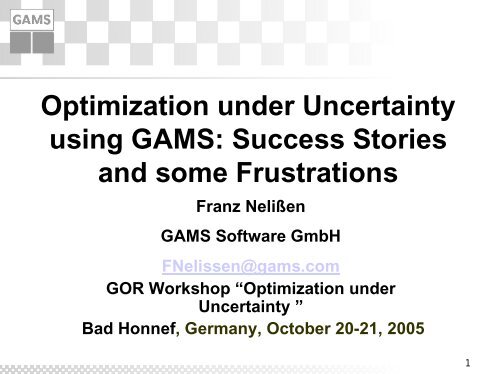
<strong>Optimization</strong> <strong>under</strong> <strong>Uncertainty</strong><br />
<strong>using</strong> <strong>GAMS</strong>: <strong>Success</strong> <strong>Stories</strong><br />
<strong>and</strong> some Frustrations<br />
Franz Nelißen<br />
<strong>GAMS</strong> Software GmbH<br />
FNelissen@gams.com<br />
GOR Workshop “<strong>Optimization</strong> <strong>under</strong><br />
<strong>Uncertainty</strong> ”<br />
Bad Honnef, Germany, October 20-21, 2005<br />
1
Overview<br />
Algebraic Modeling Languages <strong>and</strong> <strong>GAMS</strong><br />
Dealing with uncertainty<br />
Static Models: The Mean Variance Model<br />
Dynamic Models (Stochastic Programming)<br />
Summary<br />
2
<strong>GAMS</strong> Development Corp.<br />
& <strong>GAMS</strong> Software GmbH<br />
General Algebraic Modeling System<br />
Started as a research project<br />
at the World Bank 1976<br />
Went commercial in 1987<br />
Professional software tool provider<br />
Operating in a segmented niche market<br />
Broad academic <strong>and</strong> commercial user base<br />
Offices in Washington, D.C <strong>and</strong> Cologne<br />
3
Spreadsheets<br />
Modeling Tools<br />
General programming languages<br />
C++, Delphi, FORTRAN, Java, VBA, …<br />
Algebraic Modeling Languages<br />
Specialized software for certain applications<br />
Mixture of different approaches<br />
4
What are Algebraic Modeling<br />
Languages?<br />
Allow efficient h<strong>and</strong>ling of mathematical<br />
optimization problems<br />
Goals:<br />
Support the decision making process<br />
Increase productivity during model building<br />
<strong>and</strong> solution process<br />
Adapt models quickly to new situations<br />
5
Key Elements of<br />
Algebraic Modeling Languages<br />
Declarative approach<br />
Implementation of the optimization problem is close to its<br />
mathematical formulation:<br />
Variables, constraints with arbitrary names<br />
Sets, indices, algebraic expressions, powerful sparse index <strong>and</strong><br />
data h<strong>and</strong>ling<br />
Efficient but simple syntax<br />
Model formulation contains no hints how to process the<br />
model Algebraic Modeling Language translates this<br />
representation into another form suitable for the<br />
optimization algorithm<br />
Also procedural elements: Loops, procedures,<br />
macros, …<br />
6
<strong>GAMS</strong> Basic Principles<br />
Balanced mix of declarative <strong>and</strong> procedural approaches<br />
Separation of model <strong>and</strong> data: Core model is data<br />
independent <strong>and</strong> scalable<br />
Separation of model <strong>and</strong> solution methods:<br />
Multiple model types: LP, MIP, NLP, QCP, MIQCP, MINLP, MCP…<br />
Maintained links to commercial <strong>and</strong> research algorithms (open solver<br />
interface)<br />
Separation of model <strong>and</strong> operating system: Models are<br />
platform independent<br />
Open architecture <strong>and</strong> interfaces to other systems: GUI,<br />
Excel, database, programming languages etc.<br />
Maintainable models <strong>and</strong> protection of investments in<br />
models<br />
7
Typical <strong>GAMS</strong> Application Areas*<br />
Agricultural Economics<br />
Applied General Equilibrium<br />
Chemical Engineering<br />
Economic Development<br />
Econometrics<br />
Energy<br />
Environmental Economics<br />
Engineering<br />
Finance<br />
Forestry<br />
International Trade<br />
Logistics<br />
Macro Economics<br />
Military<br />
Management Science <strong>and</strong> OR<br />
Mathematics<br />
Micro Economics<br />
Physics<br />
* Illustrative examples in the <strong>GAMS</strong> Model Library<br />
8
<strong>Uncertainty</strong> in Finance<br />
Very active area with significant contributions to<br />
modeling <strong>and</strong> with important practical applications<br />
Some of the reasons:<br />
Obvious impact of uncertainty<br />
Dealing with uncertainty = Risk Management (Basel II)<br />
Real money“ - a small difference may mean a big<br />
advantage<br />
High availability of data<br />
Very competitive <strong>and</strong> liquid markets Many instruments<br />
<strong>and</strong> strategies<br />
9
<strong>Optimization</strong> Models in<br />
Finance<br />
“Static” models: The decision is made once, no<br />
further changes possible<br />
Mean-Variance Models<br />
Portfolio Models for Fixed Income<br />
Indexation Models (“Tracking Models”)<br />
Scenario based <strong>Optimization</strong><br />
“Dynamic” models: Sequence of decisions<br />
Stochastic Programming<br />
10
Mean-Variance Model<br />
Markowitz (1952)Nobel prize 1990<br />
Some investments x i with historical data:<br />
Expected returns of investments: µ i :<br />
Mean of historical returns<br />
Risk: Variance of investments Q i,j<br />
Goal: Balance risk r of portfolio against expected<br />
returns of portfolio<br />
Minimize variance v of portfolio for a given target<br />
return r<br />
11
Mean-Variance Model<br />
Min<br />
s.<br />
t.<br />
I<br />
∑∑<br />
i=<br />
1 j=<br />
1<br />
I<br />
∑<br />
i=<br />
1<br />
I<br />
∑<br />
i=<br />
1<br />
Equations<br />
Algebraic Representation:<br />
zdef.. v =g= sum((i,j), x(i)*q(i,j)*x(j));<br />
rdef.. r =e= sum(i, mu(i)*x(i));<br />
budget.. sum(i, x(i)) =e= 1;<br />
x.lo(i) = 0; # no borrowing<br />
J<br />
x<br />
i<br />
i<br />
x<br />
µ<br />
x<br />
i<br />
=<br />
i<br />
Q<br />
=<br />
1,<br />
i,<br />
j<br />
r<br />
x<br />
j<br />
x<br />
i<br />
≥<br />
0<br />
12
Mean-Variance Model<br />
Core <strong>GAMS</strong> Model<br />
$eolcom #<br />
Set i analyzed investments; alias (i,j) ;<br />
Parameter q(i,j) variance matrix;<br />
Variables v variance of portfolio,<br />
r expected return for the portfolio,<br />
x(i) fraction of the portfolio that consists<br />
of i;<br />
Equations zdef variance of portfolio<br />
rdef expected return of portfolio<br />
budget budget constraint ;<br />
zdef.. v =g= sum((i,j), x(i)*q(i,j)*x(j));<br />
rdef.. r =e= sum(i, mu(i)*x(i));<br />
budget.. sum(i, x(i)) =e= 1;<br />
13
Mean-Variance Model<br />
Data<br />
Set i / cn,fr,gr,jp,sw,uk,us /;<br />
Parameter mu(i)/<br />
cn 0.1287, fr 0.1096, gr 0.0501, jp 0.1524,<br />
sw 0.0763, uk 0.1854, us 0.0620 /;<br />
Table q(i,j)<br />
cn fr gr jp sw uk us<br />
cn 42.18<br />
fr 20.18 70.89<br />
gr 10.88 21.58 25.51<br />
jp 5.30 15.41 9.60 22.33<br />
sw 12.32 23.24 22.63 10.32 30.01<br />
uk 23.84 23.80 13.22 10.46 16.36 42.23<br />
us 17.41 12.62 4.70 1.00 7.20 9.90 16.42 ;<br />
q(i,j)$(ord(j) gt ord(i)) = q(j,i) ;<br />
14
Mean-Variance Model<br />
Procedural Elements<br />
$include data.inc # get data from external file<br />
x.lo(i) = 0; # no borrowing<br />
Model var / all / ;<br />
set p points for efficient frontier /minv, p1*p8, maxr/,<br />
pp(p) points used for loop / p1*p8 /;<br />
parameter minr , maxr, #minimal <strong>and</strong> maximal return<br />
rep(p,*), repx(p,i); # some quick reports<br />
solve var minimizing v <strong>using</strong> qcp ;#find portfolio with minimal variance<br />
rep('minv','return') = r.l; minr=r.l;<br />
rep('minv','variance') = v.l; repx('minv',i) = x.l(i);<br />
solve var maximizing r <strong>using</strong> qcp ; # find portfolio with maximal return<br />
rep('maxr','return') = r.l; maxr=r.l;<br />
rep('maxr','variance') = v.l; repx('maxr',i) = x.l(i);<br />
loop(pp, # trace efficient frontier<br />
r.fx = minr + (maxr-minr)/(card(pp)+1)*ord(pp);<br />
solve var minimizing v <strong>using</strong> qcp ;<br />
rep(pp,'return') = r.l;<br />
rep(pp,'variance') = v.l;<br />
repx(pp,i) = x.l(i);<br />
);<br />
display rep, repx;<br />
15
T arg et R etu rn o f Po rtfo lio<br />
0,2<br />
0,18<br />
0,16<br />
0,14<br />
0,12<br />
0,1<br />
0,08<br />
0,06<br />
0,04<br />
0,02<br />
0<br />
Efficient Portfolios<br />
0,00 10,00 20,00 30,00 40,00 50,00<br />
Variance of Portfolio<br />
Mean-Variance Model<br />
Solution<br />
Share<br />
100%<br />
90%<br />
80%<br />
70%<br />
60%<br />
50%<br />
40%<br />
30%<br />
20%<br />
10%<br />
0%<br />
Efficient Portfolios for Different Target Returns<br />
minv p1 p2 p3 p4 p5 p6 p7 p8 maxr<br />
Target Return of Portfolio<br />
16<br />
us<br />
uk<br />
jp<br />
gr<br />
cn
Mean-Variance Model<br />
Extensions<br />
Different risk attitudes:<br />
min λ<br />
I<br />
J<br />
∑∑<br />
i=<br />
1 j=<br />
1<br />
x<br />
Q<br />
i<br />
i,<br />
j<br />
x<br />
j<br />
− ( 1−<br />
λ)<br />
∑ xiµ<br />
i;<br />
λ ∈{<br />
0,<br />
K,<br />
1<br />
x i may become negative Allowing<br />
borrowing (Short Sales)<br />
I<br />
i=<br />
1<br />
Trading Restrictions (“Zero or Range“ –<br />
Constraints) Mixed Integer Quadratic<br />
Problem<br />
}<br />
17
Trading Restrictions- Data<br />
Table bdata(i,pd) portfolio data <strong>and</strong> trading restrictions<br />
* - increase - - decrease -<br />
old umin umax lmin lmax<br />
cn 0.2 0.03 0.11 0.03 0.11<br />
fr 0.2 0.04 0.10 0.04 0.10<br />
gr 0.0 0.04 0.07 0.04 0.07<br />
jp 0.0 0.03 0.11 0.03 0.11<br />
sw 0.2 0.03 0.20 0.03 0.20<br />
uk 0.2 0.03 0.10 0.03 0.10<br />
us 0.2 0.03 0.10 0.03 0.10<br />
;<br />
18
Trading Restrictions –<br />
Formulation<br />
Variables xi(i) fraction of portfolio increase<br />
xd(i) fraction of portfolio decrease<br />
y(i) binary switch for increasing current holdings of i<br />
z(i) binary switch for decreasing current holdings of i;<br />
Binary Variables y, z;<br />
Positive variables xi, xd;<br />
Equations xdef(i) final portfolio definition,<br />
maxinc(i) bound of maximum lot increase of fraction of i,<br />
mininc(i) bound of minimum lot increase of fraction of i,<br />
maxdec(i) bound of maximum lot decrease of fraction of i,<br />
mindec(i) bound of minimum lot decrease of fraction of i,<br />
binsum(i) restrict use of binary variables;<br />
xdef(i).. x(i) =e= bdata(i,'old') - xd(i) + xi(i);<br />
maxinc(i).. xi(i) =l= bdata(i,'umax')* y(i);<br />
mininc(i).. xi(i) =g= bdata(i,'umin')* y(i);<br />
maxdec(i).. xd(i) =l= bdata(i,'lmax')* z(i);<br />
mindec(i).. xd(i) =g= bdata(i,'lmin')* z(i);<br />
binsum(i).. y(i) + z(i) =l= 1;<br />
Model var2 /all/; Solve var2 minimizing v <strong>using</strong> miqcp ;<br />
19
Variance of Portfolio:<br />
Original: 21.419<br />
QCP, no Rest.: 9.66<br />
MIQCP: 14.853<br />
Trading Restrictions –<br />
100%<br />
90%<br />
80%<br />
70%<br />
60%<br />
50%<br />
40%<br />
30%<br />
20%<br />
10%<br />
0%<br />
Solution<br />
EfficientPortfolios<br />
Original QCP, no rest. MIQCP<br />
20<br />
us<br />
uk<br />
sw<br />
jp<br />
gr<br />
fr<br />
cn
Recent Developments<br />
Support of codes, which take advantage of<br />
special problem structures:<br />
Quadratic / Mixed Integer Quadratic<br />
Programming via Interior Point Methods / QP<br />
Simplex<br />
Support of global optimization codes<br />
21
Stochastic Programming<br />
Stochastic Programming models allow sequence of<br />
decisions<br />
Elements:<br />
Scenarios:<br />
Complete set of possible discrete realizations of the uncertain<br />
parameters with probabilities<br />
Capture complex interactions between different uncertain parameters<br />
(risk factors)<br />
What are “good scenarios”?<br />
How many scenarios are necessary?<br />
How do we generate scenarios?<br />
Stages: Decisions points. First stage decisions now, second stage<br />
decision (depending of the outcome of the first stage decision) after<br />
a certain period <strong>and</strong> so on<br />
Recourse: Describes how decision variables can adept to the<br />
different outcomes of the r<strong>and</strong>om parameters at each stage<br />
22
4<br />
A simple Scenario Tree<br />
0<br />
1 2<br />
5<br />
6 7 8<br />
combines scenarios, stages <strong>and</strong> probabilities<br />
3<br />
9<br />
Stage 1<br />
Stage 2<br />
Stage 3<br />
23
Another Scenario Tree<br />
1.8<br />
1999 2000 2001<br />
1.6<br />
2002<br />
Years<br />
3<br />
2.8<br />
2.6<br />
2.4<br />
2.2<br />
2<br />
Exchange Rate<br />
24
Stochastic Programming<br />
Some Challenges<br />
Domain specific knowledge<br />
Impacts of uncertainty:<br />
Does it make a difference <strong>and</strong> is it worth the effort?<br />
How far can one get with a certain budget?<br />
Development <strong>and</strong> Fall-Back Strategy?<br />
Data (availability <strong>and</strong> importance of certain <strong>and</strong> uncertain<br />
parameter) Generation of “good” scenarios <strong>and</strong><br />
definition of stages<br />
Interpretation <strong>and</strong> Presentation of Results<br />
Maintenance of the system<br />
25
Stochastic Programming<br />
Technical Challenges<br />
Deterministic equivalent: Includes all<br />
scenarios <strong>and</strong> stages Size of model<br />
explodes<br />
Challenges (among others):<br />
Programming <strong>and</strong> generation difficult<br />
Solution may not be possible<br />
Interpretation <strong>and</strong> validation of results<br />
26
Facing these (tech.) Challenges<br />
1. How does <strong>GAMS</strong> support the modeling of<br />
Stochastic Programming Problems?<br />
2. Some scenarios only differ slightly Can<br />
we reduce the number of scenarios?<br />
3. Stochastic Programming Problems are<br />
structured How can we take advantage<br />
of specialized solution techniques for<br />
Stochastic Programming<br />
27
Stochastic Programming in<br />
<strong>GAMS</strong><br />
Support for huge problem instances: 64 Bit OS (PC) <strong>and</strong><br />
Grid Computing (experimental)<br />
Reliable <strong>and</strong> fast import <strong>and</strong> export of data <strong>and</strong> results<br />
Visualization of results<br />
New language elements might improve reliability of :<br />
R<strong>and</strong>om distributions for some problem data<br />
Special expressions <strong>and</strong> conventions for scenario trees <strong>and</strong> stages<br />
Special sets for trees: Root, nodes, leafs, ancestor <strong>and</strong> child relations;<br />
automated generation of trees<br />
Connection of variables or constraints to certain stages: A variable or<br />
constraints is only active at a certain stage: x.stage(i)=1;<br />
28
Scenario Reduction<br />
Goal: Find an<br />
approximation of the<br />
original scenario tree<br />
with less nodes<br />
29
Scenario Reduction<br />
Steps<br />
1. Write a the stochastic model including the<br />
full tree structure<br />
2. Pass the tree structure to SCENRED*<br />
3. Reduce tree <strong>and</strong> reallocate probabilities<br />
4. Import reduced tree back to <strong>GAMS</strong><br />
5. Solve the model with the reduced tree<br />
structure<br />
* SCENRED has been developed by Groewe-Kuska, Heitsch & Römisch,<br />
Humboldt-University Berlin, Germany<br />
30
Specialized Algorithms<br />
OSL Stochastic Extensions (IBM):<br />
Solves n-stage stochastic linear<br />
programs with recourse<br />
Nested Benders decomposition<br />
Requires deterministic equivalent<br />
representation of the problem, which may<br />
be huge but is solver independent<br />
<strong>GAMS</strong> made substantial investment<br />
producing a solver independent interface,<br />
but unfortunately the product is no longer<br />
supported by IBM<br />
31
Specialized Algorithms<br />
DECIS (Infanger)<br />
Solves two-stage stochastic<br />
linear programs with recourse<br />
Benders decomposition <strong>and</strong><br />
advanced importance sampling techniques<br />
Requires additional information describing<br />
the uncertain elements of the core model in<br />
a form, which is not compatible with other<br />
solvers<br />
32
Main Problem:<br />
Specialized Algorithms<br />
No uniform (solver independent)<br />
problem representation (both for the input<br />
<strong>and</strong> output)<br />
Various approaches, not yet clear which<br />
st<strong>and</strong>ard will be adopted<br />
33
Summary<br />
Large classes of problems can be solved<br />
<strong>GAMS</strong> provides a powerful <strong>and</strong> flexible<br />
framework for these classes of models<br />
Stochastic Programming still challenging <strong>and</strong><br />
developing field<br />
Limited application of Stochastic<br />
Programming in practice<br />
34


