Using ArcToolbox™ - UNBC GIS Lab

Using ArcToolbox 

GIS by ESRI

Copyright © 1999, 2000 ESRI 

All rights reserved 

Printed in the United States of America 

The information contained in this document is the exclusive property of ESRI This work is protected under United States copyright law and other 

international copyright treaties and conventions No part of this work may be reproduced or transmitted in any form or by any means, electronic or 

mechanical, including photocopying and recording, or by any information storage or retrieval system, except as expressly permitted in writing by ESRI 

All requests should be sent to Attention: Contracts Manager, ESRI, 380 New York Street, Redlands, CA 92373-8100, USA 

The information contained in this document is subject to change without notice 

CONTRIBUTING WRITERS 

Corey Tucker, Ian DeMerchant, Barbara Bicking, Chris Boyd, Jason Pardy, Mike Conly and Ghislain Prince, Gary Kabot, and Ashley Pengelley 

US GOVERNMENT RESTRICTED/LIMITED RIGHTS 

Any software, documentation, and/or data delivered hereunder is subject to the terms of the License Agreement In no event shall the US Government 

acquire greater than RESTRICTED/LIMITED RIGHTS At a minimum, use, duplication, or disclosure by the US Government is subject to restrictions 

as set forth in FAR §52227-14 Alternates I, II, and III (JUN 1987); FAR §52227-19 (JUN 1987) and/or FAR §12211/12212 (Commercial Technical 

Data/Computer Software); and DFARS §252227-7015 (NOV 1995) (Technical Data) and/or DFARS §2277202 (Computer Software), as applicable 

Contractor/Manufacturer is ESRI, 380 New York Street, Redlands, CA 92373-8100, USA 

ESRI and the ESRI globe logo are trademarks of ESRI, registered in the United States and certain other countries; registration is pending in the European 

Community ArcInfo, ArcToolbox, ArcCatalog, AML, TABLES, ARCPLOT, ArcGIS, GIS by ESRI, the ESRI Press logo, and the ArcInfo logo are 

trademarks and wwwesricom is a service mark of ESRI The Windows logo is a trademark of Microsoft Corporation 

The names of other companies and products herein are trademarks or registered trademarks of their respective trademark owners

Quick-start tutorial 

2 

IN THIS CHAPTER 

• Exercise 1: Organizing your data 

in ArcCatalog 

• Exercise 2: Processing the forest 

stands 

• Exercise 3: Processing the 

streams and roads 

• Exercise 4: Converting data 

• Exercise 5: Creating the analysis 

coverage 

• Exercise 6: Computing the timber 

value 

Conducting a GIS processing project is easier than ever with the powerful 

tools in ArcToolbox. When used in conjunction with ArcCatalog—the application 

for browsing, storing, organizing, and distributing data—ArcToolbox lets 

you meet the geoprocessing needs of your project quickly and efficiently. 

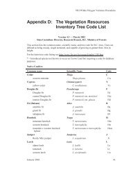
In this tutorial, you’ll use ArcToolbox and 

ArcCatalog to conduct a logging study for a 

portion of the Tongass National Forest in southeastern 

Alaska. By performing overlays, buffers, 

and other geoprocessing tasks with ArcToolbox, 

you’ll calculate the dollar value of trees in areas 

suitable for logging. You’ll use ArcCatalog to 

organize and manage your data, as well as to 

immediately preview the results for each step. 

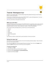
The study area is shown here. You will conduct 

the study for the PetersburgB4 and PetersburgB5 

15-minute quadrangles. You will use base coverages 

and grids for forest stands, rivers, roads, and 

old growth to complete the study. This data has been provided with the 

software. Additionally, several of the coverages you would normally derive in 

the course of this project are provided to eliminate repetitive processing steps. 

When conducting your analysis, you must keep certain study criteria in mind. 

First, harvest areas must be 100 meters from all roads and fish spawning 

streams. Second, areas must not include old growth forest. 

7

You’ll use several datasets throughout the course of the 

project. The following table provides descriptions of these 

datasets. 

Coverage 

Oldgrowgrid 

Overlay3 

Road 

Roadbuf 

Standb5 

Standddb4 

Stream 

Description 

Grid of old growth forest stands 

Overlay of buffered roads and streams, 

forest stands, and old growth forest 

Major roads 

Major roads buffered 100 meters 

Forest stands for PetersburgB5 in Universal 

Transverse Mercator (UTM) 

Forest stands for PetersburgB4 in decimal 

degrees 

Streams 

Geoprocessing Server, see ‘Using a Geoprocessing Server’ 

in Chapter 3 before you start the tutorial. 

This tutorial is designed to let you explore the capabilities of 

ArcToolbox and ArcCatalog at your own pace and without 

the need for additional assistance. You’ll need about one 

hour of focused time to complete the six exercises in the 

tutorial. However, you can also perform the exercises one 

at a time if you wish. 

The data you’ll need for this tutorial is included on the 

ArcToolbox installation disk. The datasets were provided 

courtesy of the USDA Forest Service, Tongass National 

Forest, Ketchikan Area. They have been simplified by 

ESRI. The Forest Service cannot assure the reliability or 

suitability of this information. Original data was compiled 

from various sources, and spatial information may not meet 

National Map Accuracy Standards. This information may 

be updated, corrected, or otherwise modified without notice. 

All exercises in the tutorial are processed locally, rather 

than being sent to a Geoprocessing Server for remote 

processing. It is recommended that you do not use the 

Geoprocessing Server for this tutorial if you have ArcInfo 

Workstation installed locally. If you need to use a 

8 USING ARCTOOLBOX

Exercise 1: Organizing your data in ArcCatalog 

Before you begin your geoprocessing and analysis work, 

you must first find and organize the data that you’ll need. 

You should organize your data in such a way that you’ll be 

able to find it quickly and efficiently. This will be done 

using ArcCatalog. 

Copying and connecting to data 

You’ll begin by copying the tutorial data provided with the 

ArcToolbox software to a folder on a local disk. You will 

work with a copy of the data locally if the data was installed 

on a connected disk, in order to maintain the 

integrity of the original data. Once it has been copied, you 

will then create a connection to the folder containing the 

data in ArcCatalog. 

1. Start ArcCatalog by either double-clicking a shortcut 

installed on your desktop or using the Programs list in 

your Start menu. 

2. Copy the ArcToolbox tutorial data from the directory 

where it is installed to your own tutorial workspace. In 

the examples shown here, the data has been copied to 

local drive D:\ and placed in a folder called “tutorial”. 

In ArcCatalog, data is accessed through folder connections. 

When you look in a folder connection, you can 

quickly see the folders and data sources it contains. 

You’ll now begin organizing your tutorial data by 

creating a folder connection to it. 

3. Click the Connect To Folder button and navigate to the 

data folder. Click OK to establish a folder connection. 

3 

Your new folder connection—D:\tutorial\Tongass—is 

now listed in the ArcCatalog tree. You will now be able 

to access all of the data needed for your project through 

that connection. 

Exploring your data 

Before you begin your analysis, you should explore the 

datasets provided for the project. This will help you get a 

better feel for ArcCatalog and the tutorial data. 

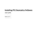
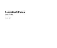
1. Click the Thumbnails button on the Standard toolbar to 

display previously created thumbnail images of the 

datasets in your Tongass folder. 

Layers have been created for all the coverages. The 

Standb5 coverage is in a UTM projection, while 

Standddb4 is in unprojected decimal degrees. All other 

coverages and grids have been merged and are in UTM 

projection. 

QUICK-START TUTORIAL 9

2 

1 

4. Right-click the VALUE-PER-METER field to open a 

context menu. Sort the table into ascending and then 

descending order. What is the lowest nonzero value per 

meter? What is the greatest? 

4 

3 

2. Click the plus sign next to the D:\tutorial\Tongass 

connection to see the datasets contained in the folder. 

Click the Preview tab and click each dataset in the tree. 

3. Double-click the Standb5 coverage to open it. Click the 

polygon feature class. Click the Preview dropdown 

arrow and click Table to see the feature attribute table 

contents. The VALUE-PER-METER field stores the 

value of the timber in each forest stand as a density— 

dollars per meter squared. 

Polygons with a value-per-meter attribute of zero are 

nonforested areas such as lakes and grasslands. Because 

the purpose of this project is to calculate the value 

of trees in areas suitable for logging, you will exclude the 

nonforested areas from the timber harvest. You will then 

compute the value of the timber in the remaining area 

using this attribute. 

Starting ArcToolbox 

In the remaining sections of the tutorial, you’ll conduct your 

geoprocessing work using ArcToolbox. You’ll still need to 

use ArcCatalog to manage and examine your datasets. 

Keep both applications open for the remainder of the 

tutorial. 

1. Click the Launch ArcToolbox button on the ArcCatalog 

toolbar to start ArcToolbox. 

1 

10 USING ARCTOOLBOX

You can also start ArcToolbox as you would any other 

application—from the Start menu or from a shortcut on 

your desktop. 

2. Both the ArcCatalog and ArcToolbox windows should 

now be open. Size and arrange the two applications on 

your screen so that both are visible. 

You are now ready to start the first part of the tutorial: 

processing the forest stands. You’ll be introduced to several 

ArcToolbox tools and wizards and will use these for your 

analysis. 


Exercise 2: Processing the forest stands 

In the first exercise, you prepared for the latter exercises 

by organizing your data. Now you are ready to begin 

processing your data. Two forest stand coverages— 

Standddb4 and Standb5—currently cover the entire study 

area. Before you can begin your study, these coverages 

must be merged. 

As noted in Exercise 1, the Standb5 coverage is projected 

in a UTM coordinate system, while the Standddb4 coverage 

is in unprojected decimal degrees. In order for you to 

conduct a meaningful analysis of these areas, the coverages 

must share the same coordinate system. For this reason, 

you will project Standddb4 to match the coordinate system 

of Standb5. Once this is done, the topology will have to be 

rebuilt as it is lost when a coverage is projected. 

Projecting a coverage 

ArcToolbox software’s Project Wizard lets you easily 

project a coverage to another coordinate system. You can 

use the Project Wizard to manually define the output 

projection (you supply all the projection parameters), or you 

can have the wizard use the projection information stored in 

an existing coverage. For this study, you’ll use the wizard to 

project the Standddb4 coverage to match the coordinate 

system of Standb5. 

1. Double-click the Project Wizard (coverages, grids) in the 

Projections toolset of Data Management Tools. 

The first panel of the Project Wizard (coverages, grids) 

should now be open. You will use the projection information 

in Standb5 to project Standddb4. 

1 

2. Click the option to Project my data to match existing 

data. Click Next. 

This panel is used to specify your input coverage. 

ArcToolbox gives you several options for setting input 

and output dataset names. You can type the full 

pathname to the dataset into the text box. You can also 

click and drag a dataset, or datasets, from the 

ArcCatalog tree or Contents tab and drop it on the text 

box. Alternatively, you can click the Browse button to 

open the ArcCatalog browser and navigate to your 

dataset. 

ArcToolbox has a feature called sticky paths. This 

means that it remembers the path to the last dataset you 

specified and will assume that the same path applies 

when you type only a dataset name into another tool or 

wizard. It also remembers output dataset paths. 

12 USING ARCTOOLBOX

Tutorial instructions will simply ask you to type coverage 

names and their paths into the appropriate text boxes. 

However, feel free to use any of the techniques just 

described to make the entry. 

3. Type “D:\tutorial\Tongass\Standddb4” in the Dataset text 

box. Click Next. 

Use the next panel of the wizard to specify the name of 

the coverage whose projection information will be used 

to define the output projection. You will use Standb5 to 

define it. Notice that in both this and the previous panel, 

the wizard displays the projection information for the 

coverage you have selected. 

4. Type “D:\tutorial\Tongass\Standb5” in the Dataset text 

box. Click Next. 

The next panel appears, where you will specify the 

output coverage name. You will call the output coverage 

“Standb4” and store it in your Tongass folder. 

5. Type “D:\tutorial\Tongass\Standb4” for the output 

dataset. Click Next. A summary page appears. Once you 

have reviewed the summary, click Finish. 

A message appears to tell you that the wizard is processing 

your request. This message appears in all tools 

and wizards when a process is active. When the tool or 

wizard is finished, the message disappears, indicating 

that the process is complete. 

Your new coverage should now appear in your Tongass 

folder. 

6. Click the Standb4 coverage in the Catalog tree and click 

the Preview tab. Switch to Geography on the Preview 

dropdown list to see your new coverage. 


Building topology 

If you double-click the Standb4 coverage in the ArcCatalog 

tree, you’ll note that the coverage doesn’t contain a polygon 

feature class. This is because changing a coverage’s 

projection removes its topology. You must now rebuild 

polygon topology for your new coverage using the Build 

tool before going any further with your analysis. 

1. Double-click the Build tool in the Topology toolset of 

Data Management Tools. 

The Standb4 and Standb5 coverages are now in the 

same projection (UTM), and your new coverage has 

polygon topology. The next step is to merge the coverages 

together so that the data can be used as one 

dataset that matches the extents of the other coverages 

in the study. 

Merging datasets 

You can use the Append Wizard to merge the two coverages. 

1. Double-click Append Wizard in the Aggregate toolset of 

Data Management Tools. 

1 

2. Type “D:\tutorial\Tongass\standb4” in the Input coverage 

text box. 

3. Change the Feature class to Poly. Click Yes on the 

subsequent message box to confirm Poly as the desired 

feature class. Click OK. 

The Append Wizard joins multiple coverages together 

when you type their names in the Coverages to be 

appended text box. The easiest way to do this is to use 

the browser and select all of the datasets at once. 

Simply click the coverage, then hold down the Ctrl or 

Shift key while clicking the other coverages to select 

them all. 

14 USING ARCTOOLBOX

2 

Use the next panel to specify the output coverage name 

and to offset the feature IDs. Unique feature IDs 

within the output coverage are necessary in order to 

maintain a relationship between the new features and 

the originals. 

7. Type “D:\tutorial\Tongass\stand” in the Output coverage 

text box. Click the Create unique IDs dropdown arrow 

and click Features only. Click Next. 

8. Review the summary panel and click Finish. 

2. Click the Browse button and navigate to the 

D:\tutorial\Tongass folder. Select Standb4 and Standb5 

and click the Open button. 

Your coverages should now be listed on the wizard. If 

you made a mistake, you can remove a coverage by 

selecting it and clicking the Delete button next to the 

list. 

3. Click Next. 

The next panel of the wizard appears. You will use it to 

specify the feature classes that will be merged. 

4. Click Poly in the Feature classes list. 


This panel is used to specify the name of an optional clip 

coverage. You will not use a clip coverage in this tutorial. 


Your forest stand data is now ready to be used with the 

other Tongass datasets in the next exercise. By analyzing 

the forest stand data along with the coverages you’ll create 

in the upcoming tasks, you will determine which areas are 

suitable for harvest and how valuable those areas are. 


Exercise 3: Processing the streams and roads 

In the last exercise, you processed the forest stands; now 

you will process the streams and roads data to eliminate the 

areas that do not meet the first of the specified criteria: 

harvest areas must be at least 100 meters from all fish 

spawning streams and roads. 

To process the streams, you will first select and extract 

stream segments flagged as fish spawning grounds and 

place them in a new coverage named Fish. You will then 

generate a 100-meter buffer around each segment. 

To meet the second part of the criterium—harvest areas 

must be at least 100 meters from roads—you would have to 

create a similar buffer. However, this step has already been 

completed for you to avoid repetition; the extracted roads 

are represented by the Roadbuf coverage. 

Extracting features 

Using the Select tool, you will extract streams that are 

flagged as fish spawning areas to a new coverage. But 

first, you should examine the stream coverage in 

ArcCatalog to see how many streams are in the study area. 

1. Click the Stream coverage in the ArcCatalog tree and 

click the Preview tab to examine the coverage. 

2. Double-click the Select tool in the Extract toolset of 

Analysis Tools. 

You will now specify the coverage and feature class that 

you are processing, the logical expression that identifies 

the features (there is a button that opens a query 

builder), and the output coverage and feature class. 

2 

3. Type “D:\tutorial\Tongass\stream” in the Input coverage 

text box. 

4. Click the Input feature class dropdown arrow and click 

Line. 

5 

3 

4 

6 

Q 

16 USING ARCTOOLBOX

5. Click the first option to Build a query if it is not already 

selected. 

6. Click the Query Builder button to open the Query 

Builder dialog box. 

You’ll use the Query Builder to create the logical 

expression that identifies the features you want to select. 

You can type the expression directly into the text box or 

build the expression by clicking the fields, operators, 

connectors, and values. You must choose the selection 

method before creating the expression, as it affects the 

expression’s logic. Once a suitable expression is created, 

you can add it to the tool’s expression list. 

The default selection method is subset. If you are 

familiar with the ArcInfo TABLES module, subset is 

the same as using the RESELECT keyword when you 

create a selection expression. 

7. Type the expression “AHMU-CLASS = 2” in the 

Current expression text box. Keep the default selection 

method. 

The item AHMU-CLASS is used to classify the stream 

types. All spawning streams have a value of 2. The 

expression tells the Select tool to extract only those 

streams with a value of 2—that is, the fish spawning 

streams. 

8. Click the down arrow button next to the Current expression 

text box to add the expression to the list. 

7 

8 

9. Click OK to close the Query Builder. 

Call your new coverage Fish and save it in your Tongass 

folder. 

10. Type “D:\tutorial\Tongass\Fish” in the Output coverage 

text box on the Select tool. Click OK. 

A message appears when the processing is complete 

asking whether you want to see the output tool messages. 

Click Yes and review the number of input and 

output lines. 

You can now view your new Fish coverage in 

ArcCatalog. 


Creating a buffer 

Now that you’ve created a coverage representing the fish 

spawning streams, you can build a 100-meter buffer around 

them using the Buffer Wizard. You’ll end up with a new 

coverage called Fishbuf. 

1. Double-click Buffer Wizard in the Proximity toolset of 


1 

regions, so accept the default buffer type and click 

Next. 

3. Type “D:\tutorial\Tongass\Fish” as the coverage you 

want to buffer. Click Next. 

4. Accept the Single buffer with Specified distance option 

and click Next. 

5. Type “100” as the buffer distance in meters and click 

Next. 

6. Click Both sides with round ends for the buffer style. 

Click Next. 

7. Type “D:\tutorial\Tongass\Fishbuf” as the output coverage. 

7 

2. Click Next after reading the introductory panel. You 

want the output coverage to contain polygons, not 

You must now set the inside and outside values for the 

output coverage. Inside and outside values are used to 

determine which areas are inside or outside the buffer 

area. 

18 USING ARCTOOLBOX

8. Type “IN-FISH” as the item name. Type “1” for the 

inside value and “0” for the outside value. Click Next 

when finished. 

9. After reviewing your choices on the last panel, click 

Finish to run the wizard. 

10. View your Fishbuf coverage in ArcCatalog. 

11. Examine the polygon attribute table for Fishbuf. Note 

the IN-FISH field and its values. Records with an IN- 

FISH value of 0 indicate a polygon that is not within 

100 meters of a stream, while records with a value of 1 

are within that distance. This item and its values will be 

important in a latter step that determines what areas are 

available for forest harvesting. 

However, to eliminate a repetitive step, the Roadbuf 

coverage was created for you. It is in your Tongass 

directory; use ArcCatalog to examine it. Pay particular 

attention to the IN-ROAD polygon attribute. 

In the next exercise, you’ll create an old growth forest 

coverage. This coverage, along with the Stand, Fishbuf, and 

Roadbuf coverages, will be used to generate the final 

results. 

As mentioned earlier, one of the timber value criteria 

requires a 100-meter buffer on major roads. To make 

this buffer, you would follow the same process you just 

followed to create the Fishbuf coverage. 


Exercise 4: Converting data 

In the previous exercises, you processed forest stands, 

streams, and roads to help in your study. Now, you’ll 

convert the grid of old growth forest areas into a coverage 

that will be used in an overlay with the forest stands. This 

grid was created exclusively for this tutorial; it was not 

provided by the Forest Service. 

You’ll use the Grid to Polygon Coverage tool to complete 

the conversion. 

1. Double-click Grid to Polygon Coverage in the Export 

from Raster toolset in Conversion Tools. 

When the tool is finished processing the request, you 

should see your new coverage, Oldgrow, in the 

ArcCatalog tree. 

1 

2. Type “D:\tutorial\Tongass\oldgrowgrid” in the Input grid 

text box. Type “D:\tutorial\Tongass\Oldgrow” in the 

Output coverage text box. Click OK. 

3. Click the Preview tab in ArcCatalog to view the 

Oldgrow coverage in Preview view. Zooming in reveals 

the common stair-step effect found in vector data that 

has been converted from raster data. 

4. Examine the attributes for the coverage’s polygon 

feature class. Areas of old growth have a GRID-CODE 

value of 1. All other areas were “Nodata” in the grid 

and have a value of -9999. When inadequate information 

is available for a cell location of a grid, the location can 

20 USING ARCTOOLBOX

e assigned a value of Nodata. Nodata and “0” are not 

the same; “0” is a valid value. Because Nodata represents 

inadequate information, Nodata cells cannot be 

used in calculating the statistics in a grid’s statistics 

(STA) table. 

You now have all the coverages you need for your 

analysis. In the next exercise, you’ll overlay them to 

create a final coverage for the study. 


Exercise 5: Creating the analysis coverage 

Now that you have organized, processed, and converted 

your data, you are ready to create the final analysis coverage. 

To create the final analysis coverage, it is necessary to 

overlay the Stand, Fishbuf, Roadbuf, and Oldgrow coverages. 

This would normally require you to perform two union 

overlays—Roadbuf with Fishbuf, and Stand with 

Oldgrow—and then intersect the two resulting coverages to 

create the final analysis coverage. 

However, to avoid repetitive tasks, you will only perform 

one union overlay—Roadbuf with Fishbuf—so that you 

can experience the Overlay wizard. The final coverage 

required for the analysis has been created for you and is 

named Overlay3. You will examine the Overlay3 coverage 

at the end of this section. 

1. Double-click Overlay Wizard in the Overlay toolset in 


2. Click the third option to Combine the polygons from 

two coverages, then click Next. 

2 

3. Type “D:\tutorial\Tongass\Fishbuf” as the input 

coverage. Click Next. 

4. Type “D:\tutorial\Tongass\Roadbuf” as the overlay 

coverage. Click Next. 

1 

22 USING ARCTOOLBOX

5. Click the option to Keep all attributes from both coverages, 

as they are needed to determine what areas are 

outside of the road and stream buffers. Click Next. 

5 

8. View the Overlay3 coverage in the Catalog. Examine 

the attribute values of the polygon attribute table. You 

should see the items you created when you buffered the 

roads and streams as well as the item created in the grid 

conversion. 

6. Type “D:\tutorial\Tongass\Overlay1” as the name of the 

output coverage. You want to use the default fuzzy 

tolerance, so click Next. 

7. Review the summary panel to ensure all input is correct. 

Click Finish when you are done. 

As mentioned, the final overlay coverage, Overlay3, was 

created for you. Overlay3 was created using the same 

procedure you just followed. All of the extra fields 

resulting from the series of overlays (Cover#, Cover-ID) 

were deleted using ArcCatalog as they are not required 

for this analysis. The items created in the buffered 

coverages and the converted grid will be used to determine 

what areas are harvestable. 

You should now have a clear understanding of the steps 

that were needed to arrive at this point. ArcToolbox broke 

down complex tasks into easy-to-follow tools and wizards, 

and ArcCatalog allowed you to immediately preview your 

results. 

With all of the geoprocessing work complete, you are ready 

for Exercise 6: Computing the timber value. 


Exercise 6: Computing the timber value 

The first five exercises focused on geoprocessing tasks. In 

this exercise, you will build on these tasks by computing the 

value of the trees in harvestable areas. These are areas 

that are not old growth and are 100 meters away from fish 

spawning streams and major roads. You will use the Select 

tool to extract the polygons that meet these criteria into a 

new coverage called Cutareas. The Statistics tool will then 

weight the VALUE-PER-METER field by the area of each 

polygon and sum the results. 

Remember that value-per-meter is a density expressing the 

value of the original stands in terms of dollars per square 

meter. Because this value is a density, it still applies even 

though the original stand polygons have been divided into 

many smaller polygons through the sequence of overlays 

that you have performed. 

Extracting the polygons 

You will begin by extracting the polygons that meet all of 

the criteria. 

1. Double-click the Select tool in the Extract toolset of 


2. Type “D:\tutorial\Tongass\Overlay3” in the Input coverage 

text box. 

3. Click the Input feature class dropdown arrow and click 

Poly. 

4. Click the Query Builder button to open the Query 

Builder dialog box. Create a logical expression to select 

all polygons that have a value not equal to 1 for the IN- 

ROAD, IN-FISH, and GRID-CODE items. The item 

that stores the old growth flag was given the name 

GRID-CODE. Remember that you can type the expression 

directly into the text box or build it by clicking the 

fields, operators, connectors, and values. Keep the 

default selection method of subset. 

3 2 

5 4 

5. Type “D:\tutorial\Tongass\Cutareas” in the Output 

coverage text box. Click OK. 

24 USING ARCTOOLBOX

1. Double-click Statistics Wizard in the Statistics toolset of 


6. Examine the Cutareas coverage in ArcCatalog. 

Visually, your new coverage is not much different from 

your Overlay3 coverage. However, in the new coverage, 

polygons that can’t be harvested now have all their attributes 

set to 0. This includes the VALUE-PER-METER 

field. You can easily verify this by opening the Cutareas 

polygon attribute table and sorting it on cutareas-id. Those 

polygons with an ID of 0—there are quite a few—didn’t 

meet your criteria. 

Generating statistics to show timber value 

The last part of this tutorial involves using the Statistics 

Wizard to compute the dollar value of the trees in each 

polygon and to get a sum of all the values. The wizard will 

do this by multiplying the polygon areas (which are in 

square meters) by the VALUE-PER-METER values 

(which are in dollars per square meter). The result will be 

written to one record in an INFO file. 

2. Click the second option to sum the contents of the valueper-meter 

item. Click Next. 

2 

3. Type “D:\tutorial\Tongass\cutareas.pat” as the input 

table. Click Next. 


4. Click the Statistical method dropdown arrow and click 

Sum. 

5. Click VALUE-PER-METER in the Item list. 

6. Check Weight item and click AREA in the list. 

4 5 6 

10. Examine your new timbervalue table in ArcCatalog 

using Preview view. What is the total value of all 

harvestable timber in the study area? If your number is 

about $2.7 billion, then you didn’t make a mistake. Trees 

are worth a lot of money! Of course, this is the value of 

almost 110 square miles of forest. 

7 

7. Click the down arrow button to add the expression to the 

list. Click Next. 

8. Click Calculate statistics for all records. Click Next. 

9. Type “D:\tutorial\Tongass\timbervalue” as the output 

table name. Click Next. Click Finish after reviewing the 

summary. 

This tutorial introduced you to the extensive capabilities of 

ArcToolbox and ArcCatalog. Using both applications, you 

quickly and easily performed a number of GIS operations 

and observed the results. You can now use these applications 

to perform your own analyses. 

You have yet to uncover many features of ArcToolbox. In 

the next few chapters, you will review all the features that 

make ArcToolbox a user-friendly and complete GIS 

application for your daily needs. 

26 USING ARCTOOLBOX

Using ArcToolbox™ - UNBC GIS Lab

You also want an ePaper? Increase the reach of your titles

Delete template?

Save as template?